Mass and Hot Baryons in Massive Galaxy Clusters from Subaru Weak Lensing and AMiBA SZE Observations

Abstract

We present a multiwavelength analysis of a sample of four hot ($T_{X}>8\,{\rm keV}$) X-ray galaxy clusters (A1689, A2261, A2142, and A2390) using joint AMiBA Sunyaev-Zel’dovich effect (SZE) and Subaru weak lensing observations, combined with published X-ray temperatures, to examine the distribution of mass and the intracluster medium (ICM) in massive cluster environments. Our observations show that A2261 is very similar to A1689 in terms of lensing properties. Many tangential arcs are visible around A2261, with an effective Einstein radius $\sim 40\arcsec$ (at $z\sim 1.5$), which when combined with our weak lensing measurements implies a mass profile well fitted by an NFW model with a high concentration $c_{\rm vir}\sim 10$, similar to A1689 and to other massive clusters. The cluster A2142 shows complex mass substructure, and displays a shallower profile $(c_{\rm vir}\sim 5)$, consistent with detailed X-ray observations which imply recent interaction. The AMiBA map of A2142 exhibits an SZE feature associated with mass substructure lying ahead of the sharp north-west edge of the X-ray core suggesting a pressure increase in the ICM. For A2390 we obtain highly elliptical mass and ICM distributions at all radii, consistent with other X-ray and strong lensing work. Our cluster gas fraction measurements, free from the hydrostatic equilibrium assumption, are overall in good agreement with published X-ray and SZE observations, with the sample-averaged gas fraction of $\langle f_{\rm gas}(<r_{200})\rangle=0.133\pm 0.027$, for our sample with $\langle M_{\rm vir}\rangle=(1.2\pm 0.1)\times 10^{15}M_{\odot}h^{-1}$. When compared to the cosmic baryon fraction $f_{b}=\Omega_{b}/\Omega_{m}$ constrained by the WMAP 5-year data, this indicates $\langle f_{\rm gas,200}\rangle/f_{b}=0.78\pm 0.16$, i.e., $(22\pm 16)$% of the baryons are missing from the hot phase of clusters.

1. Introduction

Clusters of galaxies, the largest virialized systems known, are key tracers of the matter distribution in the large scale structure of the Universe. In the standard picture of cosmic structure formation, clusters are mostly composed of dark matter (DM) as indicated by a great deal of observational evidence, with the added assumptions that DM is non relativistic (cold) and collisionless, referred to as CDM. Strong evidence for substantial DM in clusters comes from multiwavelength studies of interacting clusters (Markevitch et al., 2002), in which weak gravitational lensing of background galaxies enables us to directly map the distribution of gravitating matter in merging clusters regardless of the physical/dynamical state of the system (Clowe et al., 2006; Okabe & Umetsu, 2008). The bulk of the baryons in clusters, on the other hand, reside in the X-ray emitting intracluster medium (ICM), where the X-ray surface brightness traces the gravitational mass dominated by DM. The remaining baryons are in the form of luminous galaxies and faint intracluster light (Fukugita et al., 1998; Gonzalez et al., 2005). Since rich clusters represent high density peaks in the primordial fluctuation field, their baryonic mass fraction and its redshift dependence can in principle be used to constrain the background cosmology (e.g., Sasaki, 1996; Allen et al., 2002, 2004, 2008). In particular, the gas mass to total mass ratio (the gas fraction) in clusters can be used to place a lower limit on the cluster baryon fraction, which is expected to match the cosmic baryon fraction, $f_{b}\equiv\Omega_{b}/\Omega_{m}$. However, non-gravitational processes associated with cluster formation, such as radiative gas cooling and AGN feedback, would break the self-similarities in cluster properties, which can cause the gas fraction to acquire some mass dependence (Bialek et al., 2001; Kravtsov et al., 2005).

The deep gravitational potential wells of massive clusters generate weak shape distortions of the images of background sources due to differential deflection of light rays, resulting in a systematic distortion pattern around the centers of massive clusters, known as weak gravitational lensing (e.g., Umetsu et al., 1999; Bartelmann & Schneider, 2001). In the past decade, weak lensing has become a powerful, reliable measure to map the distribution of matter in clusters, dominated by invisible DM, without requiring any assumption about the physical/dynamical state of the system (e.g., Clowe et al., 2006; Okabe & Umetsu, 2008). Recently, cluster weak lensing has been used to examine the form of DM density profiles (e.g., Broadhurst et al., 2005b, 2008; Mandelbaum et al., 2008; Umetsu & Broadhurst, 2008), aiming for an observational test of the equilibrium density profile of DM halos and the scaling relation between halo mass and concentration, predicted by $N$-body simulations in the standard Lambda Cold Dark Matter ($\Lambda$CDM) model (Spergel et al., 2007; Komatsu et al., 2008). Observational results show that the form of lensing profiles in relaxed clusters is consistent with a continuously steepening density profile with increasing radius, well described by the general NFW model (Navarro et al., 1997), expected for collisionless CDM halos.

The Yuan-Tseh Lee Array for Microwave Background Anisotropy (Ho et al., 2008) is a platform-mounted interferometer array of up to 19 elements operating at $3\,$mm wavelength, specifically designed to study the structure of the cosmic microwave background (CMB) radiation. In the course of early AMiBA operations we conducted Sunyaev-Zel’dovich effect (SZE) observations at 94 GHz towards six massive Abell clusters with the 7-element compact array (Wu et al., 2008a). At 94 GHz, the SZE signal is a temperature decrement in the CMB sky, and is a measure of the thermal gas pressure in the ICM integrated along the line of sight (Birkinshaw, 1999; Rephaeli, 1995). Therefore it is rather insensitive to the cluster core as compared with the X-ray data, allowing us to trace the distribution of the ICM out to large radii.

This paper presents a multiwavelength analysis of four nearby massive clusters in the AMiBA sample, A1689, A2261, A2142, and A2390, for which high-quality deep Subaru images are available for accurate weak lensing measurements. This AMiBA lensing sample represents a subset of the high-mass clusters that can be selected by their high ($T_{X}>8\,$keV) gas temperatures (Wu et al., 2008a). Our joint weak lensing and SZE observations, combined with supporting X-ray information available in the published literature, will allow us to constrain the cluster gas fractions without the assumption of hydrostatic equilibrium (Myers et al., 1997; Umetsu et al., 2005), complementing X-ray based studies. Our companion papers complement details of the instruments, system performance and verification, observations and data analysis, and early science results from AMiBA. Ho et al. (2008) describe the design concepts and specifications of the AMiBA telescope. Technical aspects of the instruments are described in Chen et al. (2008) and Koch et al. (2008a). Details of the first SZE observations and data analysis are presented in Wu et al. (2008a). Nishioka et al. (2008) assess the integrity of AMiBA data with several statistical tests. Lin et al. (2008) discuss the system performance and verification. Liu et al. (2008) examine the levels of contamination from foreground sources and the primary CMB radiation. Koch et al. (2008b) present a measurement of the Hubble constant, $H_{0}$, from AMiBA SZE and X-ray data. Huang et al. (2008) discuss cluster scaling relations between AMiBA SZE and X-ray observations.

The paper is organized as follows. We briefly summarize in §2 the basis of cluster SZE and weak lensing. In §3 we present a concise summary of the AMiBA target clusters and observations. In §4 we describe our weak lensing analysis of Subaru imaging data, and derive lensing distortion and mass profiles for individual clusters. In §5 we examine and compare cluster ellipticity and orientation profiles on mass and ICM structure in the Subaru weak lensing and AMiBA SZE observations. In §6 we present our cluster models and method for measuring cluster gas fraction profiles from joint weak-lensing and SZE observations, combined with published X-ray temperature measurements; we then derive cluster gas fraction profiles, and constrain the sample-averaged gas fraction profile for our massive AMIBA-lensing clusters. Finally, a discussion and summary are given in §7.

Throughout this paper, we adopt a concordance $\Lambda$CDM cosmology with $\Omega_{m}=0.3$, $\Omega_{\Lambda}=0.7$, and $h\equiv H_{0}/(100\,{\rm km\,s^{-1}\,Mpc^{-1}})=0.7$. Cluster properties are determined at the virial radius $r_{\rm vir}$ and radii $(r_{200},r_{500},r_{2500})$, corresponding to overdensities $(200,500,2500)$ relative to the critical density of the universe at the cluster redshift.

2. Basis of Cluster Sunyaev-Zel’dovich Effect and Weak Lensing

2.1. Sunyaev-Zel’dovich Effect

We begin with a brief summary of the basic equations of the thermal SZE. Our notation here closely follows the standard notation of Rephaeli (1995).

The SZE is a spectral distortion of the CMB radiation resulting from the inverse Compton scattering of cool CMB photons by the hot ICM. The non-relativistic form of the spectral change was obtained by Sunyaev-Zel’dovich (1972) from the Kompaneets equation in the non-relativistic limit. The change in the CMB intensity $I_{\rm CMB}$ due to the SZE is written in terms of its spectral function $g$ and of the integral of the electron pressure along the line-of-sight as (Rephaeli, 1995; Birkinshaw, 1999; Carlstrom et al., 2002):

$$\Delta I_{\rm SZE}(\nu)=I_{\rm norm}\,g[x(\nu)]y(\mbox{\boldmath$\theta$}),$$ (1)

where $x(\nu)$ is the dimensionless frequency, $x\equiv h\nu/(k_{\rm B}T_{\rm CMB})\approx 1.66(\nu/94\,{\rm GHz})$, with $k_{\rm B}$ being the Boltzmann constant and $T_{\rm CMB}=2.725\,{\rm K}$ being the CMB temperature at the present-day epoch, $I_{\rm norm}=(2h/c^{3})\,(k_{\rm B}T_{\rm CMB}/h)^{2}\simeq 2.7\times 10^{8}\,{\rm Jy}\,{\rm sr}^{-1}$, and $y(\mbox{\boldmath$\theta$})$ is the Comptonization parameter defined as

$$y=\int_{-r_{\rm max}}^{+r_{\rm max}}\!dl\,\sigma_{th}n_{e}\left(\frac{k_{B}T_{e}}{m_{e}c^{2}}\right)=\frac{\sigma_{th}}{m_{e}c^{2}}\int_{-r_{\rm max}}^{+r_{\rm max}}\!dl\,\frac{\rho_{\rm gas}}{\mu_{e}m_{p}}k_{B}T_{\rm gas},$$ (2)

where $\sigma_{th}$, $m_{e}$, $c$, and $\mu_{e}$ are the Thomson cross section, the electron mass, the speed of light, and the mass per electron in units of proton mass $m_{p}$, respectively; for a fully ionized H-He plasma, $\mu_{e}=2/(1+X)\simeq 1.14$, with $X$ being the Hydrogen primordial abundance by mass fraction, $X\simeq 0.76$; $r_{\rm max}$ is the cutoff radius for an isolated cluster (see §6.3). The SZE spectral function $g(x)$ is expressed as

$$g(x)=g_{\rm NR}(x)\left[1+\delta_{\rm SZE}(x,T_{\rm gas})\right],$$ (3)

where $g_{\rm NR}(x)$ is the thermal spectral function in the non-relativistic limit (Sunyaev & Zel’dovich 1972),

$$g_{\rm NR}(x)=\frac{x^{4}e^{x}}{(e^{x}-1)^{2}}\left(x\frac{e^{x}+1}{e^{x}-1}-4\right),$$ (4)

which is zero at the cross-over frequency $x_{0}\simeq 3.83$, or $\nu_{0}=217\,$GHz, and $\delta_{\rm SZE}(x,T_{\rm gas})$ is the relativistic correction (Challinor & Lasenby, 1998; Itoh et al., 1998). The fractional intensity decrease due to the SZE with respect to the primary CMB is maximized at $\nu\sim 100\,$GHz (see Figure 1 of Zhang et al., 2002), which is well matched to the observing frequency range $86$–$102\,$GHz of AMiBA. At the central frequency $\nu_{c}=94\,$GHz of AMIBA, $g(x)\simeq-3.4$. For our hot X-ray clusters with $T_{X}=8$–$10\,{\rm keV}$, the relativistic correction to the thermal SZE is 6–7$\%$ at $\nu_{c}=94\,{\rm GHz}$.

2.2. Cluster Weak Lensing

Weak gravitational lensing is responsible for the weak shape-distortion and magnification of the images of background sources due to the gravitational field of intervening foreground clusters of galaxies and large scale structures in the universe. The deformation of the image can be described by the $2\times 2$ Jacobian matrix $\cal{A}_{\alpha\beta}$ ($\alpha,\beta=1,2$) of the lens mapping. The Jacobian ${\cal A}_{\alpha\beta}$ is real and symmetric, so that it can be decomposed as

$${\cal A}_{\alpha\beta} = (1-\kappa)\delta_{\alpha\beta}-\Gamma_{\alpha\beta},$$ (5)

$$\Gamma_{\alpha\beta} = \left(\begin{array}[]{cc}+{\gamma}_{1}&{\gamma}_{2}\\ {\gamma}_{2}&-{\gamma}_{1}\end{array}\right),$$ (8)

where $\delta_{\alpha\beta}$ is Kronecker’s delta, $\Gamma_{\alpha\beta}$ is the trace-free, symmetric shear matrix with $\gamma_{\alpha}$ being the components of spin-2 complex gravitational shear $\gamma:=\gamma_{1}+i\gamma_{2}$, describing the anisotropic shape distortion, and $\kappa$ is the lensing convergence responsible for the trace-part of the Jacobian matrix, describing the isotropic area distortion. In the weak lensing limit where $\kappa,|\gamma|\ll 1$, $\Gamma_{\alpha\beta}$ induces a quadrupole anisotropy of the background image, which can be observed from ellipticities of background galaxy images. The flux magnification due to gravitational lensing is given by the inverse Jacobian determinant,

$$\mu=\frac{1}{{\rm det}{\cal A}}=\frac{1}{(1-\kappa)^{2}-|\gamma|^{2}},$$ (9)

where we assume subcritical lensing, i.e., ${\rm det}{\cal A}(\mbox{\boldmath$\theta$})>0$.

The lensing convergence is expressed as a line-of-sight projection of the matter density contrast $\delta_{m}=(\rho_{m}-\bar{\rho})/\bar{\rho}$ out to the source plane ($s$) weighted by certain combination of co-moving angular diameter distances $r$ (e.g., Jain et al., 2000),

$$\kappa=\frac{3H_{0}^{2}\Omega_{m}}{2c^{2}}\int_{0}^{\chi_{s}}\!d\chi\,{\cal G}(\chi,\chi_{s})\frac{\delta_{m}}{a}\equiv\int\!d\Sigma_{m}\,\Sigma_{\rm crit}^{-1},$$ (10)

$${\cal G}(\chi,\chi_{s})=\frac{r(\chi)r(\chi_{s}-\chi)}{r(\chi_{s})},$$ (11)

where $a$ is the cosmic scale factor, $\chi$ is the co-moving distance, $\Sigma_{m}$ is the surface mass density of matter, $\Sigma_{m}=\int\!d\chi\,a(\rho_{m}-\bar{\rho})$, with respect to the cosmic mean density $\bar{\rho}$, and $\Sigma_{\rm crit}$ is the critical surface mass density for gravitational lensing,

$$\Sigma_{\rm crit}=\frac{c^{2}}{4\pi G}\frac{D_{s}}{D_{d}D_{ds}}$$ (12)

with $D_{s}$, $D_{d}$, and $D_{ds}$ being the (proper) angular diameter distances from the observer to the source, from the observer to the deflecting lens, and from the lens to the source, respectively. For a fixed background cosmology and a lens redshift $z_{d}$, $\Sigma_{\rm crit}$ is a function of background source redshift $z_{s}$. For a given mass distribution $\Sigma_{m}(\mbox{\boldmath$\theta$})$, the lensing signal is proportional to the angular diameter distance ratio, $D_{ds}/D_{s}$.

In the present weak lensing study we aim to reconstruct the dimensionless surface mass density $\kappa$ from weak lensing distortion and magnification data. To do this, we utilize the relation between the gradients of $\kappa$ and $\gamma$ (Kaiser, 1995; Crittenden et al., 2002),

$$\triangle\kappa(\mbox{\boldmath$\theta$})=\partial^{\alpha}\partial^{\beta}\Gamma_{\alpha\beta}(\mbox{\boldmath$\theta$})=2\hat{\cal D}^{*}\gamma(\mbox{\boldmath$\theta$})$$ (13)

where $\hat{\cal D}$ is the complex differential operator $\hat{\cal D}=(\partial_{1}^{2}-\partial_{2}^{2})/2+i\partial_{1}\partial_{2}$. The Green’s function for the two-dimensional Poisson equation is $\triangle^{-1}(\mbox{\boldmath$\theta$},\mbox{\boldmath$\theta$}^{\prime})=\ln|\mbox{\boldmath$\theta$}-\mbox{\boldmath$\theta$}^{\prime}|/(2\pi)$, so that equation (13) can be solved to yield the following non-local relation between $\kappa$ and $\gamma$ (Kaiser & Squires 1993):

$$\kappa(\mbox{\boldmath$\theta$})=\frac{1}{\pi}\int\!d^{2}\theta^{\prime}\,D^{*}(\mbox{\boldmath$\theta$}-\mbox{\boldmath$\theta$}^{\prime})\gamma(\mbox{\boldmath$\theta$}^{\prime})$$ (14)

where $D(\mbox{\boldmath$\theta$})$ is the complex kernel defined as

$$D(\mbox{\boldmath$\theta$})=\frac{\theta_{2}^{2}-\theta_{1}^{2}-2i\theta_{1}\theta_{2}}{|\theta|^{4}}.$$ (15)

Similarly, the spin-2 shear field can be expressed in terms of the lensing convergence as

$$\gamma(\mbox{\boldmath$\theta$})=\frac{1}{\pi}\int\!d^{2}\theta^{\prime}\,D(\mbox{\boldmath$\theta$}-\mbox{\boldmath$\theta$}^{\prime})\kappa(\mbox{\boldmath$\theta$}^{\prime}).$$ (16)

Note that adding a constant mass sheet to $\kappa$ in equation (16) does not change the shear field $\gamma(\mbox{\boldmath$\theta$})$ which is observable in the weak lensing limit, leading to the so-called mass-sheet degeneracy (see eq. [18]) based solely on shape-distortion measurements (e.g., Bartelmann & Schneider, 2001; Umetsu et al., 1999). In general, the observable quantity is not the gravitational shear $\gamma$ but the reduced shear,

$$g=\frac{\gamma}{1-\kappa}$$ (17)

in the subcritical regime where ${\rm det}{\cal A}>0$ (or $1/g^{*}$ in the negative parity region with ${\rm det}{\cal A}<0$). We see that the reduced shear $g$ is invariant under the following global transformation:

$$\kappa(\mbox{\boldmath$\theta$})\to\lambda\kappa(\mbox{\boldmath$\theta$})+1-\lambda,\ \ \ \gamma(\mbox{\boldmath$\theta$})\to\lambda\gamma(\mbox{\boldmath$\theta$})$$ (18)

with an arbitrary scalar constant $\lambda\neq 0$ (Schneider & Seitz, 1995).

3. AMiBA Sunyaev-Zel’dovich Effect Observations

3.1. AMIBA Telescope

The AMiBA is a dual channel 86–102 GHz (3-mm wavelength) interferometer array of up to 19-elements with dual polarization capabilities sited at 3396 m on Mauna-Loa, Hawaii (latitude: $+19.5^{\circ}$, longitude: $-155.6^{\circ}$) . AMiBA is equipped with 4-lag analog, broadband (16 GHz bandwidth centered at 94 GHz) correlators which output a set of 4 real-number correlation signals (Chen et al., 2008). These four degrees of freedom (dof) correspond to two complex visibilities in two frequency channels. The frequency of AMiBA operation was chosen to take advantage of the optimal frequency window at 3 mm, where the fractional decrement in the SZE intensity relative to the primary CMB is close to its maximum (see §2.1) and contamination by the Galactic synchrotron emission, dust foregrounds, and the population of cluster/background radio sources is minimized (see for detailed contamination analysis, Liu et al., 2008). This makes AMiBA a unique CMB/SZE interferometer, and also complements the wavelength coverage of other existing and planned CMB instruments: interferometers such as AMI at 15 GHz (Kneissl et al., 2001), CBI at 30 GHz (Padin et al., 2001, 2002; Mason et al., 2003; Pearson et al., 2003), SZA at 30 and 90 GHz (Mroczkowski et al., 2008), and VSA at 34 GHz (Watson et al., 2003); bolometer arrays such as ACT, APEX-SZ (Halverson et al., 2008), and SPT.

In the initial operation of AMiBA, we used seven 0.6 m (0.58 m to be precise) Cassegrain antennas (Koch et al., 2006) co-mounted on a 6 m hexapod platform in a hexagonal close-packed configuration (see Ho et al., 2008). At each of the frequency channels centered at about 90 and 98 GHz, this compact configuration provides 21 simultaneous baselines with three baseline lengths of $d=0.61$, 1.05, and 1.21 m, corresponding to angular multipoles $l=2\pi\sqrt{u^{2}+v^{2}}(=2\pi d/\lambda)$ of $l\approx 1194,2073,2394$ at $\nu_{c}=94\,{\rm GHz}$. This compact 7-element array is sensitive to multipole range $800\lower 2.15277pt\hbox{$\;\buildrel<\over{\sim}\;$}l\lower 2.15277pt\hbox{$\;\buildrel<\over{\sim}\;$}2600$. With 0.6-m antennas, the instantaneous field-of-view of AMiBA is about $23^{\prime}$ FWHM (Wu et al., 2008a), and its angular resolution ranges from $2^{\prime}$ to $6^{\prime}$ depending on the configuration and weighting scheme. In the compact configuration, the angular resolution of AMiBA is about $6^{\prime}$ FWHM using natural weighting (i.e., inverse noise variance weighting). The point source sensitivity is estimated to be $\sim 63\,$mJy (Lin et al., 2008) in 1 hour of on-source integration in 2-patch main-trail/lead differencing observations, where the overall noise level is increased by a factor of $\sqrt{2}$ due to the differencing.

3.2. Initial Target Clusters

The AMiBA lensing sample, A1689, A2142, A2261, A2390, is a subset of the AMiBA cluster sample (see Wu et al., 2008a), composed of four massive clusters at relatively low redshifts of $0.09\lower 2.15277pt\hbox{$\;\buildrel<\over{\sim}\;$}z\lower 2.15277pt\hbox{$\;\buildrel<\over{\sim}\;$}0.23$ with the median redshift of $\bar{z}\approx 0.2$. The sample size is simply limited by the availability of high quality Subaru weak lensing data. A1689 is a relaxed, round system, and is one of the best studied clusters for lensing work (e.g., Broadhurst et al., 2005b; Limousin et al., 2007; Umetsu & Broadhurst, 2008; Broadhurst et al., 2008). A2261 is a compact cluster with a regular X-ray morphology. A2142 is a merging cluster with two sharp X-ray surface brightness discontinuities in the cluster core (Markevitch et al., 2000; Okabe & Umetsu, 2008). A2390 shows an elongated morphology both in the X-ray emission and strong-lensing mass distributions (Allen et al., 2001; Frye & Broadhurst, 1998). Table Mass and Hot Baryons in Massive Galaxy Clusters from Subaru Weak Lensing and AMiBA SZE Observations summarizes the physical properties of the four target clusters in this multiwavelength study.

In 2007, AMiBA with the seven small antennas (henceforth AMiBA7) was in the science verification phase. For our initial observations, we therefore selected those target clusters observable from Mauna Loa during the observing period that were known to have strong SZEs at relatively low redshifts ($0.1\lower 2.15277pt\hbox{$\;\buildrel<\over{\sim}\;$}z\lower 2.15277pt\hbox{$\;\buildrel<\over{\sim}\;$}0.3$) from previous experiments, such as OVRO observations at 30 GHz (Mason et al., 2001), BIMA/OVRO observations at 30 GHz (Grego et al., 2001a; Reese et al., 2002), VSA observations at 34 GHz (Lancaster et al., 2005), and SuZIE II observations at 145, 221, and 355 GHz (Benson et al., 2004). The targeted redshift range allows the target clusters to be resolved by the $6^{\prime}$ resolution of AMiBA7, allowing us to derive useful measurements of cluster SZE profiles for our multiwavelength studies. At redshifts of $z\lower 2.15277pt\hbox{$\;\buildrel<\over{\sim}\;$}0.3$ (0.2), the angular resolution of AMiBA7 corresponds to $\lower 2.15277pt\hbox{$\;\buildrel<\over{\sim}\;$}560\,{\rm kpc}h^{-1}$ ($\sim 400\,{\rm kpc}h^{-1}$) in radius, which is $\lower 2.15277pt\hbox{$\;\buildrel<\over{\sim}\;$}30$–$40\%$ ($\sim 20$–$30\%$) of the virial radius 1.5–2$\,{\rm Mpc}h^{-1}$ of massive clusters. The requirement of being SZE strong is to ensure reliable SZE measurements at 3 mm with AMiBA7. We note that AMiBA and SZA are the only SZE instruments measuring at 3 mm, but complimentary in their baseline coverage. With sensitivities of 20–30 mJy beam^-1 typically achieved in 2-patch differencing observations in 5–10 hours of net on-source integration (Wu et al., 2008a), we would expect $\lower 2.15277pt\hbox{$\;\buildrel>\over{\sim}\;$}5\sigma$ detections of SZE fluxes $\lower 2.15277pt\hbox{$\;\buildrel>\over{\sim}\;$}100$–$150\,$mJy at 3 mm. Finally, our observing period (April–August 2007) limited the range of right ascension (RA) of targets, since we restricted our science observations to nights (roughly 8pm to 8am), where we would expect high gain stability because the ambient temperature varies slowly and little (Nishioka et al., 2008). The SZE strong clusters in our AMiBA sample are likely to have exceedingly deep potential wells, and indeed our AMiBA sample represents a class of hot X-ray clusters with observed X-ray temperatures exceeding $8\,{\rm keV}$ (see Table Mass and Hot Baryons in Massive Galaxy Clusters from Subaru Weak Lensing and AMiBA SZE Observations ). We note that this may affect the generality of the results presented in this study. A main-trail/lead differencing scheme has been used in our targeted cluster observations where the trail/lead (blank) field is subtracted from the main (cluster) field. This differencing scheme sufficiently removes contamination from ground spillover and electronic DC offset in the correlator output (Wu et al., 2008a). A full description of AMiBA observations and analysis of the initial six target clusters, including the observation strategy, analysis methodology, calibrations, and map-making, can be found in Wu et al. (2008a, b).

4. Subaru Weak Lensing Data and Analysis

In this section we present a technical description of our weak lensing distortion analysis of the AMiBA lensing sample based on Subaru data. The present work on A1689 is based on the same Subaru images as analyzed in our earlier work of Broadhurst et al. (2005b) and Umetsu & Broadhurst (2008), but our improved color selection of the red background has increased the sample size by $\sim 16\%$ (§4.3). This work on A2142 is based on the same Subaru images as in Okabe & Umetsu (2008), but our inclusion of blue, as well as red, galaxies has increased the sample size by a factor of $4$ (cf. Table 6 of Okabe & Umetsu 2008), leading to a significant improvement of our lensing measurements. For A2261 and A2390 we present our new weak lensing analysis based on Suprime-Cam imaging data retrieved from the Subaru archive, SMOKA. The reader only interested in the main result may skip directly to §4.4.

4.1. Subaru Data and Photometry

We analyze deep images of four high mass clusters in the AMiBA sample taken by the wide-field camera Suprime-Cam ($34^{\prime}\times 27^{\prime}$; Miyazaki et al., 2002) at the prime-focus of the 8.3m Subaru telescope. The clusters were observed deeply in two optical passbands each with seeing in the co-added images ranging from $0.55\arcsec$ to $0.88\arcsec$ (see Table 2). For each cluster we select an optimal combination of two filters that allows for an efficient separation of cluster/background galaxies based on color-magnitude correlations (see Table 2). We use either $R_{\rm c}$ or $i^{\prime}$ band for our weak lensing measurements (described in §4.2) for which the instrumental response, sky background and seeing conspire to provide the best-quality images. The standard pipeline reduction software for Suprime-Cam (Yagi et al., 2002) is used for flat-fielding, instrumental distortion correction, differential refraction, sky subtraction and stacking. Photometric catalogs are constructed from stacked and matched images using SExtractor (Bertin & Arnouts, 1996), and used for our color selection of background galaxies (see §4.3).

4.2. Weak Lensing Distortion Analysis

We use the IMCAT package developed by N. Kaiser to perform object detection, photometry and shape measurements, following the formalism outlined in Kaiser et al. (1995, KSB). Our analysis pipeline is implemented based on the procedures described in Erben et al. (2001) and on verification tests with STEP1 data of mock ground-based observations (Heymans et al., 2006). The same analysis pipeline has been used in Umetsu & Broadhurst (2008), Okabe & Umetsu (2008), and Broadhurst et al. (2008).

4.2.1 Object Detection

Objects are first detected as local peaks in the image by using the IMCAT hierarchical peak-finding algorithm hfindpeaks which for each object yields object parameters such as a peak position ($x$), an estimate of the object size ($r_{g}$), the significance of the peak detection ($\nu$). The local sky level and its gradient are measured around each object from the mode of pixel values on a circular annulus defined by inner and outer radii of $16\times r_{g}$ and $32\times r_{g}$. In order to avoid contamination in the background estimation by bright neighboring stars and/or foreground galaxies, all pixels within $3\times r_{g}$ of another object are excluded from the mode calculation. Total fluxes and half-light radii ($r_{h}$) are then measured on sky-subtracted images using a circular aperture of radius $3\times r_{g}$ from the object center. Any pixels within $2.5\times r_{g}$ of another object are excluded from the aperture. The aperture magnitude is then calculated from the measured total flux and a zero-point magnitude. Any objects with positional differences between the peak location and the weighted-centroid greater than $|\mbox{\boldmath$d$}|=0.4$ pixels are excluded from the catalog.

Finally, bad objects such as spikes, saturated stars, and noisy detections need to be removed from the weak lensing analysis. We removed from our detection catalog extremely small or large objects with $r_{g}<1$ or $r_{g}>10$ pixels, objects with low detection significance, $\nu<7$ (see Erben et al., 2001), objects with large raw ellipticities, $|e|>0.5$ (see §4.2.2), noisy detections with unphysical negative fluxes, and objects containing more than $10$ bad pixels, ${\it nbad}>10$.

4.2.2 Weak Lensing Distortion Measurements

To obtain an estimate of the reduced shear, $g_{\alpha}=\gamma_{\alpha}/(1-\kappa)$ ($\alpha=1,2$), we measure using the getshapes routine in IMCAT the image ellipticity $e_{\alpha}=\left\{Q_{11}-Q_{22},Q_{12}\right\}/(Q_{11}+Q_{22})$ from the weighted quadrupole moments of the surface brightness of individual galaxies defined in the above catalog,

$$Q_{\alpha\beta}=\int\!d^{2}\theta\,W({\theta})\theta_{\alpha}\theta_{\beta}I({\mbox{\boldmath$\theta$}})\ \ \ (\alpha,\beta=1,2)$$ (19)

where $I(\mbox{\boldmath$\theta$})$ is the surface brightness distribution of an object, $W(\theta)$ is a Gaussian window function matched to the size of the object, and the object center is chosen as the coordinate origin. In equation (19) the maximum radius of integration is chosen to be $\theta_{\rm max}=4r_{g}$.

Firstly the PSF anisotropy needs to be corrected using the star images as references:

$$e^{\prime}_{\alpha}=e_{\alpha}-P_{sm}^{\alpha\beta}q^{*}_{\beta}$$ (20)

where $P_{sm}$ is the smear polarizability tensor (which is close to diagonal), and $q^{*}_{\alpha}=(P_{sm}^{*})^{-1}_{\alpha\beta}e_{*}^{\beta}$ is the stellar anisotropy kernel. We select bright, unsaturated foreground stars identified in a branch of the half-light radius vs. magnitude diagram to measure $q^{*}_{\alpha}$. In order to obtain a smooth map of $q^{*}_{\alpha}$ which is used in equation (20), we divided the co-added mosaic image (of $\sim 10{\rm K}\times 8{\rm K}$ pixels) into rectangular blocks. The block length is based on the coherent scale of PSF anisotropy patterns, and is typically $2{\rm K}\,$pixels. In this way the PSF anisotropy in individual blocks can be well described by fairly low-order polynomials. We then fitted the $q^{*}$ in each block independently with second-order bi-polynomials, $q_{*}^{\alpha}(\mbox{\boldmath$\theta$})$, in conjunction with iterative outlier rejection on each component of the residual: $\delta e^{*}_{\alpha}=e^{*}_{\alpha}-(P_{sm}^{*})^{\alpha\beta}q^{*}_{\beta}(\mbox{\boldmath$\theta$})$. The final stellar sample contains typically 500–1200 stars. Uncorrected ellipticity components of stellar objects have on average a mean offset (from a value of zero) of 1–2$\%$ with a few $\%$ of rms, or variation of PSF across the data field (see, e.g., Umetsu & Broadhurst, 2008; Okabe & Umetsu, 2008). On the other hand, the mean residual stellar ellipticity $\overline{\delta e^{*}_{\alpha}}$ after correction is less than or about $10^{-4}$, with the standard error on this measurement, a few $\times 10^{-4}$. We show in Figure 1 the quadrupole PSF anisotropy fields as measured from stellar ellipticities before and after the anisotropic PSF correction for our target clusters. Figure 2 shows the distributions of stellar ellipticity components before and after the PSF anisotropy correction. In addition, we adopt a conservative magnitude limit $m<25.5$–$26.0$ ABmag, depending on the depth of the data for each cluster, to avoid systematic errors in the shape measurement (see Umetsu & Broadhurst, 2008). From the rest of the object catalog, we select objects with $r_{h}>\overline{r_{h}^{*}}+\sigma(r_{h}^{*})$ pixels as a magnitude-selected weak lensing galaxy sample, where $\overline{r_{h}^{*}}$ is the median value of stellar half-light radii $r_{h}^{*}$, corresponding to half the median width of the circularized PSF over the data field, and $\sigma(r_{h}^{*})$ is the rms dispersion of $r_{h}^{*}$.

Second, we need to correct image ellipticities for the isotropic smearing effect caused by atmospheric seeing and the window function used for the shape measurements. The pre-seeing reduced shear $g_{\alpha}$ can be estimated from

$$g_{\alpha}=(P_{g}^{-1})_{\alpha\beta}e^{\prime}_{\beta}$$ (21)

with the pre-seeing shear polarizability tensor $P^{g}_{\alpha\beta}$ defined as Hoekstra et al. (1998),

$$P^{g}_{\alpha\beta}=P^{sh}_{\alpha\beta}-\left[P^{sm}(P^{sm*})^{-1}P^{sh*}\right]_{\alpha\beta}\approx P^{sh}_{\alpha\beta}-P^{sm}_{\alpha\beta}\frac{{\rm tr}[P^{sh*}]}{{\rm tr}[P^{sm*}]}$$ (22)

with $P^{sh}$ being the shear polarizability tensor; In the second equality we have used a trace approximation to the stellar shape tensors, $P^{sh*}$ and $P^{sm*}$. To apply equation (21) the quantity ${\rm tr}[P^{sh*}]/{\rm tr}[P^{sm*}]$ must be known for each of the galaxies with different sizescales. Following Hoekstra et al. (1998), we recompute the stellar shapes $P^{sh*}$ and $P^{sm*}$ in a range of filter scales $r_{g}$ spanning that of the galaxy sizes ($r_{g}=[1,10]\,$pixels). At each filter scale $r_{g}$, the median $\langle{\rm tr}[P^{sh*}]/{\rm tr}[P^{sm*}]\rangle$ over the stellar sample is calculated, and used in equation (22) as an estimate of ${\rm tr}[P^{sh*}]/{\rm tr}[P^{sm*}]$. Further, we adopt a scalar correction scheme, namely

$$(P_{g})_{\alpha\beta}=\frac{1}{2}{\rm tr}[P_{g}]\delta_{\alpha\beta}\equiv P^{\rm s}_{g}\delta_{\alpha\beta}$$ (23)

(Erben et al., 2001; Hoekstra et al., 1998; Umetsu & Broadhurst, 2008). In order to suppress artificial effects due to the noisy $P_{g}^{\rm s}$ estimated for individual galaxies, we apply filtering to raw $P_{g}^{\rm s}$ measurements. We compute for each object a median value of $P_{g}^{\rm s}$ among $N$-neighbors in the size and magnitude plane to define the object parameter space: firstly, for each object, $N$-neighbors with raw $P_{g}^{\rm s}>0$ are identified in the size ($r_{g}$) and magnitude plane; the median value of $P_{g}^{\rm s}$ is then used as the smoothed $P_{g}^{\rm s}$ for the object, $\langle P_{g}^{\rm s}\rangle$, and the variance $\sigma^{2}_{g}$ of $g=g_{1}+ig_{2}$ is calculated using equation (21). The dispersion $\sigma_{g}$ is used as an rms error of the shear estimate for individual galaxies. We take $N=30$. Finally, we use the estimator $g_{\alpha}=e^{\prime}_{\alpha}/\left<P_{g}^{\rm s}\right>$ for the reduced shear.

4.3. Background Selection

It is crucial in the weak lensing analysis to make a secure selection of background galaxies in order to minimize contamination by unlensed cluster/foreground galaxies and hence to make an accurate determination of the cluster mass profile; otherwise dilution of the distortion signal arises from the inclusion of unlensed galaxies, particularly at small radius where the cluster is relatively dense (Broadhurst et al., 2005b; Medezinski et al., 2007). This dilution effect is simply to reduce the strength of the lensing signal when averaged over a local ensemble of galaxies, in proportion to the fraction of unlensed galaxies whose orientations are randomly distributed, thus diluting the lensing signal relative to the reference background level derived from the background population Medezinski et al. (2007).

To separate cluster members from the background and hence minimize the weak lensing dilution, we follow an objective background selection method developed by Medezinski et al. (2007) and Umetsu & Broadhurst (2008). We select red galaxies with colors redder than the color-magnitude sequence of cluster E/S0 galaxies. The sequence forms a well defined line in object color-magnitude space due to the richness and relatively low redshifts of our clusters. These red galaxies are expected to lie in the background by virtue of $k$-corrections which are greater than for the red cluster sequence galaxies; This has been convincingly demonstrated spectroscopically by Rines & Geller (2008). We also include blue galaxies falling far from the cluster sequence to minimize cluster contamination.

Figure 3 shows for each cluster the mean distortion strength averaged over a wide radial range of $\theta=[1^{\prime},18^{\prime}]$ as a function of color limit, done separately for the blue (left) and red (right) samples, where the color boundaries for the present analysis are indicated by vertical dashed lines for respective color samples. Here we do not apply area weighting to enhance the effect of dilution in the central region (see Umetsu & Broadhurst, 2008). A sharp drop in the lensing signal is seen when the cluster red sequence starts to contribute significantly, thereby reducing the mean lensing signal. Note that the background populations do not need to be complete in any sense but should simply be well defined and contain only background. For A1689, the weak lensing signal in the blue sample is systematically lower than that of the red sample, so that blue galaxies in A1689 are excluded from the present analysis, as was done in Umetsu & Broadhurst (2008); on the other hand, our improved color selection for the red sample has led to a $\sim 16\%$ increase of red galaxies. In the present study we use for A2142 the same Subaru images as analyzed by Okabe & Umetsu (2008), but we have improved significantly our lensing measurements by including blue, as well as red, galaxies, where the sample size has been increased by a factor of 4.

An estimate of the background depth is required when converting the observed lensing signal into physical mass units, because the lensing signal depends on the source redshifts in proportion to $D_{ds}/D_{s}$. The mean depth is sufficient for our purposes as the variation of the lens distance ratio, $D_{ds}/D_{s}$, is slow for our sample because the clusters are at relatively low redshifts ($z_{d}\sim 0.1-0.2$) compared to the redshift range of the background galaxies. We estimate the mean depth $\langle D_{ds}/D_{s}\rangle$ of the combined red+blue background galaxies by applying our color-magnitude selection to Subaru multicolor photometry of the HDF-N region (Capak et al., 2004) or the COSMOS deep field (Capak et al., 2007), depending on the availability of filters. The fractional uncertainty in the mean depth $\langle D_{ds}/D_{s}\rangle$ for the red galaxies is typically $\sim 3\%$, while it is about $5\%$ for the blue galaxies. It is useful to define the distance-equivalent source redshift $z_{s,D}$ (Medezinski et al., 2007; Umetsu & Broadhurst, 2008) defined as

$$\bigg{\langle}\frac{D_{ds}}{D_{s}}\bigg{\rangle}_{z_{s}}=\frac{D_{ds}}{D_{s}}\bigg{|}_{z_{s}=z_{s,D}}.$$ (24)

We find $z_{s,D}=0.70^{+0.06}_{-0.05},0.95^{+0.79}_{-0.30},0.98^{+0.24}_{-0.16},1.00^{+0.25}_{-0.16}$ for A1689, A2142, A2261, and A2390, respectively. For the nearby cluster A2142 at $z\simeq 0.09$, a precise knowledge of the source redshift is not critical at all for lensing work. The mean surface number density ($n_{g}$) of the combined blue+red sample, the blue-to-red fraction of background galaxies (B/R), the estimated mean depth $\langle D_{ds}/D_{s}\rangle$, and the effective source redshift $z_{s,D}$ are listed in Table 2.

4.4. Weak Lensing Map-Making

Weak lensing measurements of the gravitational shear field can be used to reconstruct the underlying projected mass density field. In the present study, we will use the dilution-free, color-selected background sample (§4.3) both for the 2D mass reconstruction and the lens profile measurements.

Firstly, we pixelize distortion data of background galaxies into a regular grid of pixels using a Gaussian $w_{g}(\theta)\propto\exp[-\theta^{2}/\theta_{f}^{2}]$ with $\theta_{f}={\rm FWHM}/\sqrt{4\ln{2}}$. Further we incorporate in the pixelization a statistical weight $u_{g}$ for an individual galaxy, so that the smoothed estimate of the reduced shear field at an angular position $\theta$ is written as

$$\bar{g}_{\alpha}(\mbox{\boldmath$\theta$})=\frac{\sum_{i}w_{g}(\mbox{\boldmath$\theta$}-\mbox{\boldmath$\theta$}_{i})u_{g,i}g_{\alpha,i}}{\sum_{i}w_{g}(\mbox{\boldmath$\theta$}-\mbox{\boldmath$\theta$}_{i})u_{g,i}}$$ (25)

where $g_{\alpha,i}$ is the reduced shear estimate of the $i$th galaxy at angular position $\mbox{\boldmath$\theta$}_{i}$, and $u_{g,i}$ is the statistical weight of $i$th galaxy taken as the inverse variance, $u_{g,i}=1/(\sigma_{g,i}^{2}+\alpha^{2})$, with $\sigma_{g,i}$ being the rms error for the shear estimate of $i$th galaxy (see § 4.2.2) and $\alpha^{2}$ being the softening constant variance (Hamana et al., 2003). We choose $\alpha=0.4$, which is a typical value of the mean rms $\bar{\sigma}_{g}$ over the background sample. The case with $\alpha=0$ corresponds to an inverse-variance weighting. On the other hand, the limit $\alpha\gg\sigma_{g,i}$ yields a uniform weighting. We have confirmed that our results are insensitive to the choice of $\alpha$ (i.e., inverse-variance or uniform weighting) with the adopted smoothing parameters. The error variance for the smoothed shear $\bar{g}=\bar{g}_{1}+i\bar{g}_{2}$ (25) is then given as

$$\sigma^{2}_{\bar{g}}(\mbox{\boldmath$\theta$})=\frac{\sum_{i}w_{g,i}^{2}u_{g,i}^{2}\sigma^{2}_{g,i}}{\left(\sum_{i}w_{g,i}u_{g,i}\right)^{2}}$$ (26)

where $w_{g.i}=w_{g}(\mbox{\boldmath$\theta$}-\mbox{\boldmath$\theta$}_{i})$ and we have used $\langle g_{\alpha,i}\,g_{\beta,j}\rangle=(1/2)\sigma_{g,i}^{2}\delta^{\rm K}_{\alpha\beta}\delta^{\rm K}_{ij}$ with $\delta^{\rm K}_{\alpha\beta}$ and $\delta_{ij}^{\rm K}$ being the Kronecker’s delta.

We then invert the pixelized reduced-shear field (25) to obtain the lensing convergence field $\kappa(\mbox{\boldmath$\theta$})$ using equation (14). In the map-making we assume linear shear in the weak-lensing limit, that is, $g_{\alpha}=\gamma_{\alpha}/(1-\kappa)\approx\gamma_{\alpha}$. We adopt the Kaiser & Squires inversion method (Kaiser & Squires, 1993), which makes use of the 2D Green function in an infinite space (§2.2). In the linear map-making process, the pixelized shear field is weighted by the inverse of the variance (26). Note that this weighting scheme corresponds to using only the diagonal part of the noise covariance matrix, $N(\mbox{\boldmath$\theta$}_{i},\mbox{\boldmath$\theta$}_{j})=\langle\overline{\Delta g}(\mbox{\boldmath$\theta$}_{i})\overline{\Delta g}(\mbox{\boldmath$\theta$}_{j})\rangle$, which is only an approximation of the actual inverse noise weighting in the presence of pixel-to-pixel correlation due to non-local Gaussian smoothing. In Table 2 we list the rms noise level in the reconstructed $\kappa(\mbox{\boldmath$\theta$})$ field for our sample of target clusters. For all of the clusters, the smoothing scale $\theta_{f}$ is taken to be $\theta_{f}=1\arcmin$ ($\theta_{\rm FWHM}\simeq 1.665\arcmin$), which is larger than the Einstein radius for our background galaxies. Hence our weak lensing approximation here is valid in all clusters.

In Figure 4 we show, for the four clusters, 2D maps of the lensing convergence $\kappa(\mbox{\boldmath$\theta$})=\Sigma_{m}(\mbox{\boldmath$\theta$})/\Sigma_{\rm crit}$ reconstructed from the Subaru distortion data (§4.4), each with the corresponding gravitational shear field overlaid. Here the resolution of the $\kappa$ field is $\sim 1.665\arcmin$ in FWHM for all of the four clusters. The side length of the displayed region is $22\arcmin$, corresponding roughly to the instantaneous field-of-view of AMiBA ($\simeq 23\arcmin$ in FWHM). In the absence of higher-order effects, weak lensing only induces curl-free $E$-mode distortions, responsible for tangential shear patterns, while the $B$-mode lensing signal is expected to vanish. For each case, a prominent mass peak is visible in the cluster center, around which the lensing distortion pattern is clearly tangential.

Also shown in Figure 4 are contours of the AMiBA flux density due to the thermal SZE obtained by Wu et al. (2008a). The resolution of AMiBA7 is about $6^{\prime}$ in FWHM (§3). The AMiBA map of A1689 reveals a bright and compact structure in the SZE, similar to the compact and round mass distribution reconstructed from the Subaru distortion data. A2142 shows an extended structure in the SZE elongated along the northwest-southeast direction, consistent with the direction of elongation of the X-ray halo, with its general cometary appearance (Markevitch et al., 2000). In addition, A2142 shows a slight excess in SZE signals located $\sim 10\arcmin$ northwest of the cluster center, associated with mass substructure seen in our lensing $\kappa$ map (Figure 4); This slight excess SZE appears extended for a couple of synthesized beams, although the per-beam significance level is marginal ($2-3\sigma$). Okabe & Umetsu (2008) showed that this northwest mass substructure is also associated with a slight excess of cluster sequence galaxies, lying $\sim 5\arcmin$ ahead of the northwest edge of the central X-ray gas core. On the other hand, no X-ray counterpart to the northwest substructure was found in the X-ray images from Chandra and XMM-Newton observations (Okabe & Umetsu, 2008). A2261 shows a filamentary mass structure with unknown redshift, extending to the west of the cluster core (Maughan et al., 2008), and likely background structures which coincide with redder galaxy concentrations (see §4.5.2 for details). Our AMiBA and Subaru observations show a compact structure both in mass and ICM. The elliptical mass distribution in A2390 agrees well with the shape seen by AMiBA in the thermal SZE, and is also consistent with other X-ray and strong lensing work. A quantitative comparison between the AMiBA SZE and Subaru lensing maps will be given in §5.

4.5. Cluster Lensing Profiles

4.5.1 Lens Distortion

The spin-2 shape distortion of an object due to gravitational lensing is described by the complex reduced shear, $g=g_{1}+ig_{2}$ (see equation [17]), which is coordinate dependent. For a given reference point on the sky, one can instead form coordinate-independent quantities, the tangential distortion $g_{+}$ and the $45^{\circ}$ rotated component, from linear combinations of the distortion coefficients $g_{1}$ and $g_{2}$ as

$$g_{+}=-(g_{1}\cos 2\phi+g_{2}\sin 2\phi),\ \ g_{\times}=-(g_{2}\cos 2\phi-g_{1}\sin 2\phi),$$ (27)

where $\phi$ is the position angle of an object with respect to the reference position, and the uncertainty in the $g_{+}$ and $g_{\times}$ measurement is $\sigma_{+}=\sigma_{\times}=\sigma_{g}/\sqrt{2}\equiv\sigma$ in terms of the rms error $\sigma_{g}$ for the complex shear measurement. In practice, the reference point is taken to be the cluster center, which is well determined by the locations of the brightest cluster galaxies. To improve the statistical significance of the distortion measurement, we calculate the weighted average of $g_{+}$ and $g_{\times}$, and its weighted error, as

$$\langle g_{+}(\theta_{m})\rangle = \frac{\sum_{i}u_{g,i}\,g_{+,i}}{\sum_{i}u_{g,i}},$$ (28)

$$\langle g_{\times}(\theta_{m})\rangle = \frac{\sum_{i}u_{g,i}\,g_{\times,i}}{\sum_{i}u_{g,i}},$$ (29)

$$\sigma_{+}(\theta_{m}) = \sigma_{\times}(\theta_{m})=\sqrt{\frac{\sum_{i}u^{2}_{g,i}\sigma^{2}_{i}}{\left(\sum_{i}u_{g,i}\right)^{2}},}$$ (30)

where the index $i$ runs over all of the objects located within the $m$th annulus with a median radius of $\theta_{m}$, and $u_{g,i}$ is the inverse variance weight for $i$th object, $u_{g,i}=1/(\sigma_{g,i}^{2}+\alpha^{2})$, softened with $\alpha=0.4$ (see §4.4).

Now we assess cluster lens-distortion profiles from the color-selected background galaxies (§4.3) for the four clusters, in order to examine the form of the underlying cluster mass profile and to characterize cluster mass properties. In the weak lensing limit ($\kappa,|\gamma|\ll 1$), the azimuthally averaged tangential distortion profile $\langle g_{+}(\theta)\rangle$ (eq. [28]) is related to the projected mass density profile (e.g., Bartelmann & Schneider, 2001) as

$$\langle g_{+}(\theta)\rangle\simeq\langle\gamma_{+}(\theta)\rangle=\bar{\kappa}(<\theta)-\langle\kappa(\theta)\rangle,$$ (31)

where $\langle\cdots\rangle$ denotes the azimuthal average, and $\bar{\kappa}(<\theta)$ is the mean convergence within a circular aperture of radius $\theta$ defined as $\bar{\kappa}(<\theta)=(\pi\theta^{2})^{-1}\int_{|\mbox{\boldmath$\theta$}^{\prime}|\leq\theta}\!d^{2}\theta^{\prime}\,\kappa(\mbox{\boldmath$\theta$}^{\prime})$. Note that equation (31) holds for an arbitrary mass distribution. With the assumption of quasi-circular symmetry in the projected mass distribution, one can express the tangential distortion as $\langle g_{+}(\theta)\rangle\simeq[\bar{\kappa}(<\theta)-\langle\kappa(\theta)\rangle]/[1-\langle\kappa(\theta)\rangle]$ in the non-linear but sub-critical (${\rm det}{\cal A}(\mbox{\boldmath$\theta$})>0$) regime.

Figure 5 shows the azimuthally-averaged radial profiles of the tangential distortion, $\langle g_{+}\rangle$ ($E$ mode), and the $45^{\circ}$-rotated component, $\langle g_{\times}\rangle$ ($B$ mode). Here the presence of $B$ modes can be used to check for systematic errors. For each of the clusters, the observed $E$-mode signal is significant at the $12$–$16\sigma$ level out to the limit of our data ($\theta\sim 20^{\prime}$). The significance level of the $B$-mode detection is about $2.5\sigma$ for each cluster, which is about a factor of $5$ smaller than $E$-mode.

The measured $g_{+}$ profiles are compared with two representative cluster mass models, namely the NFW model and the singular isothermal sphere (SIS) model. Firstly, the NFW universal density profile has a two-parameter functional form as

$$\rho_{\rm NFW}(r)=\frac{\rho_{s}}{(r/r_{s})(1+r/r_{s})^{2}},$$ (32)

where $\rho_{s}$ is a characteristic inner density, and $r_{s}$ is a characteristic inner radius. The logarithmic gradient $n\equiv d\ln\rho(r)/d\ln r$ of the NFW density profile flattens continuously towards the center of mass, with a flatter central slope $n=-1$ and a steeper outer slope ($n\to-3$ when $r\to\infty$) than a purely isothermal structure ($n=-2$). A useful index, the concentration, compares the virial radius, $r_{\rm vir}$, to $r_{s}$ of the NFW profile, $c_{\rm vir}=r_{\rm vir}/r_{s}$. We specify the NFW model with the halo virial mass $M_{\rm vir}$ and the concentration $c_{\rm vir}$ instead of $\rho_{s}$ and $r_{s}$. We employ the radial dependence of the NFW lensing profiles, $\kappa_{\rm NFW}(\theta)$ and $\gamma_{+,{\rm NFW}}(\theta)$, given by Bartelmann (1996) and Wright & Brainerd (2000). Next, the SIS density profile is given by

$$\rho_{\rm SIS}(r)=\frac{\sigma_{v}^{2}}{2\pi Gr^{2}},$$ (33)

where $\sigma_{v}$ is the one-dimensional isothermal velocity dispersion of the SIS halo. The lensing profiles for the SIS model, obtained by projections of the three-dimensional mass distribution, are found to be

$$\kappa_{\rm SIS}(\theta)=\gamma_{+,{\rm SIS}}(\theta)=\frac{\theta_{E}}{2\theta},$$ (34)

where $\theta_{E}$ is the Einstein radius defined by $\theta_{E}\equiv 4\pi(\sigma_{v}/c)^{2}D_{ds}/D_{s}$.

Table 3 lists the best-fitting parameters for these models, together with the predicted Einstein radius $\theta_{\rm E}$ for a fiducial source at $z_{s}=1.5$, corresponding roughly to the median redshifts of our blue background galaxies. For a quantitative comparison of the models, we introduce as a measure of the goodness-of-fit the significance probability $Q(\nu/2,\chi^{2}/2)$ to find by chance a value of $\chi^{2}$ as poor as the observed value for a given number of dof, $\nu$ (see §15.2 in Press et al., 1992). We find with our best-fit NFW models $Q$-values of $Q\simeq 0.50,0.95,0.36$, and $0.80$, and with our best-fit SIS models $Q\simeq 0.28,5.0\times 10^{-6},0.37$, and $0.87$, for A1689, A2142, A2261, and A2390, respectively. Both models provide statistically acceptable fits for A1689, A2261, and A2390. For our lowest-$z$ cluster A2142, the curvature in the $g_{+}$ profile is pronounced, and a SIS model for A2142 is strongly ruled out by the Subaru distortion data alone, where the minimum $\chi^{2}$ is $\chi^{2}_{\rm min}=39$ with 8 dof.

4.5.2 Lens Convergence

Although the lensing distortion is directly observable, the effect of substructure on the gravitational shear is non-local. Here we examine the lens convergence ($\kappa$) profiles using the shear-based 1D reconstruction method developed by Umetsu & Broadhurst (2008). See Appendix A.1 for details of the reconstruction method.

In Figure 6 we show, for the four clusters, model-independent $\kappa$ profiles derived using the shear-based 1D reconstruction method, together with predictions from the best-fit NFW models for the $\kappa(\theta)$ and $g_{+}(\theta)$ data. The substructure contribution to $\kappa(\theta)$ is local, whereas the inversion from the observable distortion to $\kappa$ involves a non-local process. Consequently the 1D inversion method requires a boundary condition specified in terms of the mean $\kappa$ value within an outer annular region (lying out to $18^{\prime}$–$19^{\prime}$). We determine this value for each cluster using the best-fit NFW model for the $g_{+}$ profile (Table 3).

We find that the two sets of best-fit NFW parameters are in excellent agreement for all except A2261: For A2261, the best-fit values of $c_{\rm vir}$ from the $g_{+}$ and $\kappa$ profiles are are in poorer agreement. From Figures 4 and 6 we see that the NFW fit to the $g_{+}$ profile of A2261 is affected by the presence of mass structures at outer radii, $\theta\simeq 4^{\prime}$ and $10^{\prime}$, resulting in a slightly shallower profile ($c_{\rm vir}\simeq 6.4$) than in the $\kappa$ analysis. It turns out that these mass structures are associated with galaxy overdensities whose mean colors are redder than the cluster sequence for A2261 at $z=0.224$, $\Delta(V-R_{\rm c})\equiv(V-R_{\rm c})-(V-R_{\rm c})_{A2261}\sim+0.6$, and hence they are likely to be physically unassociated background objects. The NFW fit to $\kappa(\theta)$ yields a steeper profile with a high concentration, $c_{\rm vir}\simeq 10.2$, which implies a large Einstein angle of $\theta_{\rm E}\simeq 37\arcsec$ at $z_{s}=1.5$ (Table 3). This is in good agreement with our preliminary strong-lensing model (Zitrin et al. in preparation) based on the method by Broadhurst et al. (2005a), in which the deflection field is constructed based on the smoothed cluster light distribution to predict the appearance and positions of counter images of background galaxies. This model is refined as new multiply-lensed images are identified in deep Subaru $VR_{\rm c}$ and CFHT/WIRCam $JHK_{s}$ images, and incorporated to improve the cluster mass model. Figure 7 shows the tangential critical curve predicted for a background source at $z_{s}\sim 1.5$, overlaid on the Subaru $V+R_{\rm c}$ pseudo-color image in the central $6.7^{\prime}\times 6.7^{\prime}$ region of A2261. The predicted critical curve is a nearly circular Einstein ring, characterized by an effective radius of $\theta_{\rm E}\sim 40\arcsec$ (see Oguri & Blandford, 2008). This motivates us to further improve the statistical constraints on the NFW model by combining the outer lens convergence profile with the observed constraint on the inner Einstein radius. A joint fit of the NFW profile to the $\kappa$ profile and the inner Einstein-radius constraint with $\theta_{\rm E}=40\arcsec\pm 4\arcsec$ ($z_{s}=1$) tightens the constraints on the NFW parameters (see §5.4.2 of Umetsu & Broadhurst 2008): $M_{\rm vir}=1.25^{+0.17}_{-0.16}\times 10^{15}M_{\odot}h^{-1}$ and $c_{\rm vir}=11.1^{+2.2}_{-1.9}$; This model yields an Einstein radius of $\theta_{E}=(40\pm 11)\arcsec$ at $z_{s}=1.5$. In the following analysis we will adopt this as our primary mass model of A2261.

For the strong-lensing cluster A1689, more detailed lensing constraints are available from joint observations with the high-resolution Hubble Space Telescope (HST) Advanced Camera for Surveys (ACS) and the wide-field Subaru/Suprime-Cam (Broadhurst et al., 2005b; Umetsu & Broadhurst, 2008). In Umetsu & Broadhurst (2008) we combined all possible lensing measurements, namely, the ACS strong-lensing profile of Broadhurst et al. (2005b) and Subaru weak-lensing distortion and magnification data, in a full two-dimensional treatment, to achieve the maximum possible lensing precision. Note, the combination of distortion and magnification data breaks the mass-sheet degeneracy (see eq. [18]) inherent in all reconstruction methods based on distortion information alone (Bartelmann et al., 1996). It was found that the joint ACS and Subaru data, covering a wide range of radii from 10 up to 2000 kpc$\,h^{-1}$, are well approximated by a single NFW profile with $M_{\rm vir}=(1.5\pm 0.1^{+0.6}_{-0.3})\times 10^{15}M_{\odot}h^{-1}$ and $c_{\rm vir}=12.7\pm 1\pm 2.8$ (statistical followed by systematic uncertainty at 68$\%$ confidence). This properly reproduces the Einstein radius, which is tightly constrained by detailed strong-lens modeling (Broadhurst et al., 2005a; Halkola et al., 2006; Limousin et al., 2007): $\theta_{\rm E}\simeq 52\arcsec$ at $z_{s}=3.05$ (or $\theta_{\rm E}\simeq 45\arcsec$ at a fiducial source redshift of $z_{s}=1$). With the improved color selection for the red background sample (see §4.3), we have redone a joint fit to the ACS and Subaru lensing observations using the 2D method of Umetsu & Broadhurst (2008): The refined constraints on the NFW parameters are $M_{\rm vir}=1.55^{+0.13}_{-0.12}\times 10^{15}M_{\odot}h^{-1}$ and $c_{\rm vir}=12.3^{+0.9}_{-0.8}$, yielding an Einstein radius of $50^{+6.5}_{-6.0}$ arcsec at $z_{s}=1.5$. In the following, we will adopt this refined NFW profile as our primary mass model of A1689.

5. Distributions of Mass and Hot Baryons

Here we aim to compare the projected distribution of mass and ICM in the clusters using our Subaru weak lensing and AMiBA SZE maps. To make a quantitative comparison, we first define the “cluster shapes” on weak lensing mass structure by introducing a spin-2 halo ellipticity $e^{\rm halo}=e_{1}^{\rm halo}+ie_{2}^{\rm halo}$, defined in terms of weighted quadrupole shape moments $Q_{\alpha\beta}^{\rm halo}$ ($\alpha,\beta=1,2$), as

$$e^{\rm halo}_{\alpha}(\theta_{\rm ap}) = \left(\frac{Q^{\rm halo}_{11}-Q^{\rm halo}_{22}}{Q^{\rm halo}_{11}+Q^{\rm halo}_{22}},\frac{2Q^{\rm halo}_{12}}{Q^{\rm halo}_{11}+Q^{\rm halo}_{22}}\right),$$ (35)

$$Q^{\rm halo}_{\alpha\beta}(\theta_{\rm ap}) = \int_{\Delta\theta\leq\theta_{\rm ap}}\!d^{2}\theta\,\Delta\theta_{\alpha}\Delta\theta_{\beta}\,\kappa(\mbox{\boldmath$\theta$}),$$ (36)

where $\theta_{\rm ap}$ is the circular aperture radius, and $\Delta\theta_{\alpha}$ is the angular displacement vector from the cluster center. Similarly, the spin-2 halo ellipticity for the SZE is defined using the cleaned SZE decrement map $-\Delta I(\mbox{\boldmath$\theta$})\propto y(\mbox{\boldmath$\theta$})$ instead of $\kappa(\mbox{\boldmath$\theta$})$ in equation (36). The degree of halo ellipticity is quantified by the modulus of the spin-2 ellipticity, $|e^{\rm halo}|=\sqrt{(e_{1}^{\rm halo})^{2}+(e_{2}^{\rm halo})^{2}}$, and the orientation of halo is defined by the position angle of the major axis, $\phi^{\rm halo}=\arctan(e_{2}^{\rm halo}/e_{1}^{\rm halo})/2$. In order to avoid noisy shape measurements, we introduce a lower limit of $\kappa(\mbox{\boldmath$\theta$})>0$ and $-\Delta I(\mbox{\boldmath$\theta$})>0$ in equation (36). Practical shape measurements are done using pixelized lensing and SZE maps shown in Figure 4. The images are sufficiently oversampled that the integral in equation (36) can be approximated by the discrete sum. Note, a comparison in terms of the shape parameters is optimal for the present case where the paired AMiBA and weak lensing images have different angular resolutions: $\theta_{\rm FWHM}\simeq 6\arcmin$ FWHM for AMiBA7, and $\theta_{\rm FWHM}\simeq 1.7\arcmin$ FWHM for Subaru weak lensing. When the aperture diameter is larger than the resolution $\theta_{\rm FWHM}$, i.e., $\theta_{\rm ap}>\theta_{\rm FWHM}/2$, the halo shape parameters can be reasonably defined and measured from the maps.

Now we measure as a function of aperture radius $\theta_{\rm ap}$ the cluster ellipticity and orientation profiles for projected mass and ICM pressure as represented by the lensing $\kappa$ and SZE decrement maps, respectively. For the Subaru weak lensing, the shape parameters are measured at $\theta_{\rm ap}=[1,2,3,...,11]\times\theta_{\rm FWHM}$ ($1.7\arcmin\lower 2.15277pt\hbox{$\;\buildrel<\over{\sim}\;$}\theta_{\rm ap}\lower 2.15277pt\hbox{$\;\buildrel<\over{\sim}\;$}18.3\arcmin)$; for the AMiBA SZE, $\theta_{\rm ap}=[1,2,3]\times\theta_{\rm FWHM}$ ($6\arcmin\lower 2.15277pt\hbox{$\;\buildrel<\over{\sim}\;$}\theta_{\rm ap}\lower 2.15277pt\hbox{$\;\buildrel<\over{\sim}\;$}18\arcmin)$. The level of uncertainty in the halo shape parameters is assessed by a Monte-Carlo error analysis assuming Gaussian errors for weak lensing distortion and AMiBA visibility measurements (for the Gaussianity of AMiBA data, see Nishioka et al., 2008). For each cluster and dataset, we generate a set of 500 Monte Carlo simulations of Gaussian noise and propagate into final uncertainties in the spin-2 halo ellipticity, $e^{\rm halo}$. Figure 8 displays, for the four clusters, the resulting cluster ellipticity and orientation profiles on mass and ICM structure as measured from the Subaru weak lensing and AMiBA SZE maps, shown separately for the ellipticity modulus $|e^{\rm halo}|$ and the orientation, $2\phi^{\rm halo}$ (twice the position angle). Overall, a good agreement is found between the shapes of mass and ICM structure up to large radii, in terms of both ellipticity and orientation. In particular, our results on A2142 and A2390 show that the mass and pressure distributions trace each other well at all radii. At a large radius of $\theta_{\rm ap}\lower 2.15277pt\hbox{$\;\buildrel>\over{\sim}\;$}10^{\prime}$, the position angle of A2142 is $\phi^{\rm halo}\sim 50^{\circ}$. For A2390, the position angle is $\phi^{\rm halo}\sim 30^{\circ}$ at all radii.

6. Cluster Gas Mass Fraction Profiles

6.1. Method

In modeling the clusters, we consider two representative analytic models for describing the cluster DM and ICM distributions, namely (1) the Komatsu & Seljak (2001, hereafter KS01) model of the universal gas density/temperature profiles and (2) the isothermal $\beta$ model, where both are physically motivated under the hypothesis of hydrostatic equilibrium and polytropic equation-of-state, $P\propto\rho^{\gamma}$, with an additional assumption about the spherical symmetry of the system.

Joint AMiBA SZE and Subaru weak lensing observations probe cluster structures on angular scales up to $\Delta\theta\sim 23\arcmin$. At the median redshift $\bar{z}\simeq 0.2$ of our clusters, this maximum angle covered by the data corresponds roughly to $r_{200}\approx 0.8r_{\rm vir}$, except $r_{500}\approx 0.5r_{\rm vir}$ for A2142 at $z=0.09$. In order to better constrain the gas mass fraction in the outer parts of the clusters, we adopt a prior that the gas density profile $\rho_{\rm gas}(r)$ traces the underlying (total) mass density profile, $\rho_{\rm tot}(r)$. Such a relationship is expected at large radii, where non-gravitational processes, such as radiative cooling and star formation, have not had a major effect on the structure of the atmosphere so that the polytropic assumption remains valid (Lewis et al. 2000). Clearly this results in the gas mass fraction, $\rho_{\rm gas}(r)/\rho_{\rm tot}(r)$, tending to a constant at large radius. In the context of the isothermal $\beta$ model, this simply means that $\beta=2/3$.

In both models, for each cluster, the mass density profile $\rho_{\rm tot}(r)$ is constrained solely by the Subaru weak lensing data (§4), the gas temperature profile $T_{\rm gas}(r)$ is normalized by the spatially-averaged X-ray temperature (see Table Mass and Hot Baryons in Massive Galaxy Clusters from Subaru Weak Lensing and AMiBA SZE Observations ), and the electron pressure profile $P_{e}(r)=n_{e}(r)k_{B}T_{e}(r)$ is normalized by the AMiBA SZE data, where $n_{e}(r)$ is the electron number density, and $T_{e}(r)=T_{\rm gas}(r)$ is the electron temperature. The gas density is then given by $\rho_{\rm gas}(r)=\mu_{e}m_{p}n_{e}(r)$.

6.2. Cluster Models

6.2.1 NFW-Consistent Model of Komatsu & Seljak 2001

The KS01 model describes the polytropic gas in hydrostatic equilibrium with a gravitational potential described by the universal density profile for collisionless CDM halos proposed by Navarro et al. (1996, hereafter NFW). See KS01, Komatsu & Seljak (2002, hereafter KS02), and Worrall & Birkinshaw (2006) for more detailed discussions. High mass clusters with virial masses $M_{\rm vir}\lower 2.15277pt\hbox{$\;\buildrel>\over{\sim}\;$}10^{15}M_{\odot}/h$ are so massive that the virial temperature of the gas is too high for efficient cooling and hence the cluster potential simply reflects the dominant DM. This has been recently established by our Subaru weak lensing study of several massive clusters (Broadhurst et al., 2005b, 2008; Umetsu & Broadhurst, 2008).

In this model, the gas mass profile traces the NFW profile in the outer region of the halo ($r_{\rm vir}/2\lower 2.15277pt\hbox{$\;\buildrel<\over{\sim}\;$}r\lower 2.15277pt\hbox{$\;\buildrel<\over{\sim}\;$}r_{\rm vir}$; see KS01), satisfying the adopted prior of the constant gas mass fraction $\rho_{\rm gas}(r)/\rho_{\rm tot}(r)$ at large radii. This behavior is supported by cosmological hydrodynamic simulations (e.g., Yoshikawa et al., 2000), and is recently found from the stacked SZE analysis of the WMAP 3-year data (Atrio-Barandela et al., 2008). The shape of the gas distribution functions, as well as the polytropic index $\gamma_{\rm gas}$, can be fully specified by the halo virial mass, $M_{\rm vir}$, and the halo concentration, $c_{\rm vir}=r_{\rm vir}/r_{s}$, of the NFW profile.

In the following, we use the form of the NFW profile to determine $r_{\rm vir}$, $r_{200}$, $r_{500}$, and $r_{2500}$. Table 4 summarizes the NFW model parameters derived from our lensing analysis for the four clusters (see §4.5). For each cluster we also list the corresponding $(r_{2500},r_{500},r_{200},r_{\rm vir})$. For calculating $\gamma_{\rm gas}$ and the normalization factor $\eta(0)$ for a structure constant ($B$ in equation [16] of KS02), we follow the fitting formulae given by KS02, which are valid for halo concentration, $1<c_{\rm vir}<25$ (see Table 4). For our clusters, $\gamma_{\rm gas}$ is in the range of $1.15$ to $1.20$. Following the prescription in KS01, we convert the X-ray cluster temperature $T_{X}$ to the central gas temperature $T_{\rm gas}(0)$ of the KS01 model.

6.2.2 Isothermal $\beta$ Profile

The isothermal $\beta$ model provides an alternative consistent solution of the hydrostatic equilibrium equation (Hattori et al., 1999), assuming the ICM is isothermal and its density profile follows $\rho_{\rm gas}(r)=\rho_{\rm gas}(0)[1+(r/r_{c})^{2}]^{-3\beta/2}$ with the gas core radius $r_{c}$. At large radii, $r\gg r_{c}$, where both of our SZE and weak lensing observations are sensitive, the total mass density follows $\rho_{\rm tot}(r)\propto r^{-2}$. Thus we set $\beta=2/3$ to satisfy our assumption of constant $\rho_{\rm gas}(r)/\rho_{\rm tot}(r)$ at large radius. We adopt the values of $r_{c}$ and $T_{X}$ listed in Table Mass and Hot Baryons in Massive Galaxy Clusters from Subaru Weak Lensing and AMiBA SZE Observations , taken from X-ray observations, and use $T_{\rm gas}(r)=T_{X}$ as the gas temperature for this model. At $r\gg r_{c}$, the $\rho_{\rm tot}(r)$ profile can be approximated by that of a SIS (see §4.5.1) parametrized by the isothermal 1D velocity dispersion $\sigma_{v}$ (see Table 4), constrained by the Subaru distortion data (see §4.5).

Requiring hydrostatic balance gives an isothermal temperature $T_{\rm SIS}$, equivalent to $\sigma_{v}$, as

$$k_{B}T_{\rm SIS}\equiv\mu m_{p}\sigma_{v}^{2}\frac{2}{3\beta}.$$ (37)

For $\beta=2/3$, $k_{B}T_{\rm SIS}=\mu m_{p}\sigma_{v}^{2}$, which can be compared with the observed $T_{X}$ (Table Mass and Hot Baryons in Massive Galaxy Clusters from Subaru Weak Lensing and AMiBA SZE Observations ). For our AMiBA-lensing cluster sample, we found X-ray to SIS temperature ratios $T_{X}/T_{\rm SIS}=0.82\pm 0.03,1.65\pm 0.15,0.94\pm 0.05,1.28\pm 0.15$ for A1689, A2142, A2261, and A2390, respectively. For A2261 and A2390, the inferred temperature ratios are consistent with unity at 1–2$\sigma$. For the merging cluster A2142, the observed spatially-averaged X-ray temperature (cooling-flow corrected; see Markevitch, 1998) is significantly higher than the lensing-derived temperature. This temperature excess of $\sim 4\sigma$ could be explained by the effects of merger boosts, as discussed in Okabe & Umetsu (2008). The temperature ratio $T_{X}/T_{\rm SIS}$ for A1689, on the other hand, is significantly lower than unity. Recently, a similar level of discrepancy was also found in Lemze et al. (2008a), who performed a careful joint X-ray and lensing analysis of this cluster. A deprojected 3D temperature profile was obtained using a model-independent approach to the Chandra X-ray emission measurements and the projected mass profile obtained from the joint strong/weak lensing analysis of Broadhurst et al. (2005b). The projected temperature profile predicted from their joint analysis exceeds the observed temperature by $30\%$ at all radii, a level of discrepancy suggested from hydrodynamical simulations that find that denser, more X-ray luminous small-scale structure can bias X-ray temperature measurements downward at about the same level (Kawahara et al., 2007). If we accept this $+30\%$ correction for $T_{X}$, the ratio $T_{X}/T_{\rm SIS}\rightarrow 1.07\pm 0.04$ for A1689, consistent with $\beta=2/3$.

6.3. AMiBA SZE Data

We use our AMiBA data to constrain the remaining normalization parameter for the $\rho_{\rm gas}(r)$ profile, $\rho_{\rm gas}(0)$. The calibrated output of the AMiBA interferometer, after the lag-to-visibility transformation (Wu et al., 2008a), is the complex visibility $V(\mbox{\boldmath$u$})$ as a function of baseline vector in units of wavelength, $\mbox{\boldmath$u$}=\mbox{\boldmath$d$}/\lambda$, given as the Fourier transform of the sky brightness distribution $\Delta I(\mbox{\boldmath$\theta$})$ attenuated by the antenna primary beam pattern $A(\mbox{\boldmath$\theta$})$.

In targeted AMiBA observations at 94 GHz, the sky signal $\Delta I(\mbox{\boldmath$\theta$})$ with respect to the background (i.e., atmosphere and the mean CMB intensity) is dominated by the thermal SZE due to hot electrons in the cluster, $\Delta I_{\rm SZE}=I_{\rm norm}\,g(\nu)y$ (see eq. [1]). The Comptonization parameter $y$ is expressed as a line-of-sight integral of the thermal electron pressure (see eq. [2]). In the line-of-sight projection of equation (2), the cutoff radius $r_{\rm max}$ needs to be specified. We take $r_{\rm max}\equiv\alpha_{r}r_{\rm vir}$ with a dimensionless constant $\alpha_{r}$ which we set to $\alpha_{r}=2$. In the present study we found the line-of-sight projection in equation (2) is insensitive to the choice of $\alpha_{r}$ as long as $\alpha_{r}\lower 2.15277pt\hbox{$\;\buildrel>\over{\sim}\;$}1$.

A useful measure of the thermal SZE is the integrated Comptonization parameter $Y(\theta)$,

$$Y(\theta)=2\pi\int_{0}^{\theta}\!d\theta^{\prime}\,\theta^{\prime}y(\theta^{\prime}),$$ (38)

which is proportional to the SZE flux, and is a measure of the thermal energy content in the ICM. The value of $Y$ is less sensitive to the details of the model fitted than the central Comptonization parameter $y_{0}\equiv y(0)$, with the current configuration of AMiBA. If the $A(\mbox{\boldmath$\theta$})y(\mbox{\boldmath$\theta$})$ field has reflection symmetry about the pointing center, then the imaginary part of $V(\mbox{\boldmath$u$})$ vanishes, and the sky signal is entirely contained in the real visibility flux. If the $A(\mbox{\boldmath$\theta$})y(\mbox{\boldmath$\theta$})$ field is further azimuthally symmetric, the real visibility flux is expressed by the Hankel transform of order zero as

$$V^{Re}(u) = 2\pi I_{\rm norm}g(\nu_{c})\int_{0}^{\infty}\!d\theta\,\theta A(\theta)y(\theta)J_{0}(2\pi u\theta)$$ (39)

$$\equiv 2\pi I_{0}\int_{0}^{\infty}\!d\theta\,\theta A(\theta)\frac{y(\theta)}{y_{0}}J_{0}(2\pi u\theta),$$

where $I_{0}=I_{\rm norm}g(\nu_{c})y_{0}$ is the central SZE intensity at $\nu_{c}=94\,$GHz, $J_{0}(x)$ is the Bessel function of the first kind and order zero, and $A(\theta)$ is well approximated by a circular Gaussian with ${\rm FWHM}=1.22(\lambda/D)\simeq 23\arcmin$ at $\nu_{c}=94{\rm GHz}$ with an antenna diameter of $D=60{\rm cm}$ (Wu et al., 2008a). The observed imaginary flux can be used to check for the effects of primary CMB and radio source contamination (Liu et al., 2008). From our AMiBA data we derive in the Fourier domain azimuthally-averaged visibility profiles $\langle V(u)\rangle$ for individual clusters.

We constrain the normalization $I_{0}$ from $\chi^{2}$ fitting to the $\langle V(u)\rangle$ profile (Liu et al., 2008). In order to convert $I_{0}$ into the central Comptonization parameter, we take account of (i) the relativistic correction $\delta_{\rm SZE}(\nu,T_{\rm gas})$ in the SZE spectral function $g(\nu)$ (see eq. [3]) and (ii) corrections for contamination by discrete radio point sources (Liu et al., 2008). The level of contamination in $I_{0}$ from known discrete point sources has been estimated to be about $(6-35)\%$ in our four clusters (Liu et al., 2008). In all cases, a net positive contribution of point sources was found in our 2-patch differencing AMiBA observations (§3), indicating that there are more radio sources towards clusters than in the background (Liu et al., 2008). Thus ignoring the point source correction would systematically bias the SZE flux estimates, leading to an underestimate of $y_{0}$. The relativistic correction to the thermal SZE is 6–7$\%$ in our $T_{X}$ range at $94\,$GHz.

Table 5 summarizes, for our two models, the best-fitting parameter, $y_{0}$, and the $Y$-parameter interior to a cylinder of radius $\theta=3\arcmin$ that roughly matches the AMiBA synthesized beam with $6^{\prime}$ FWHM. For each case, both cluster models yield consistent values of $y_{0}$ and $Y(3^{\prime})$ within $1\sigma$; in particular, the inferred values of $Y(3^{\prime})$ for the two models are in excellent agreement. Following the procedure in §6.1 we convert $y_{0}$ into the central gas mass density, $\rho_{\rm gas}(0)$.

6.4. Gas Mass Fraction Profiles

We derive cumulative gas fraction profiles,

$$f_{\rm gas}(<r)=\frac{M_{\rm gas}(<r)}{M_{\rm tot}(<r)},$$ (40)

for our cluster sample using two sets of cluster models described in §6.2, where $M_{\rm gas}(<r)$ and $M_{\rm tot}(<r)$ are the hot gas and total cluster masses contained within a spherical radius $r$. In Table 6 we list, for each of the clusters, $M_{\rm gas}$ and $f_{\rm gas}$ within $r_{2500},$$r_{500}$, and $r_{200}$ (see also Table 4) calculated with the two models. Note that our total mass estimates do not require the assumption of hydrostatic balance, but are determined based solely on the weak lensing measurements. Gaussian error propagation was used to derive the errors on $M_{\rm gas}(<r)$ and $f_{\rm gas}(<r)$. We propagate errors on the individual cluster parameters (Tables Mass and Hot Baryons in Massive Galaxy Clusters from Subaru Weak Lensing and AMiBA SZE Observations and 4) by a Monte-Carlo method. For A2142, the isothermal model increasingly overpredicts $f_{\rm gas}$ at all radii $r>r_{2500}$, exceeding the cosmic baryon fraction $f_{b}=\Omega_{b}/\Omega_{m}=0.171\pm 0.009$ (Dunkley et al., 2008). For other clusters in our sample, both cluster models yield consistent $f_{\rm gas}$ and $M_{\rm gas}$ measurements within the statistical uncertainties from the SZE and weak lensing data.

Our SZE/weak lensing-based measurements can be compared with other X-ray and SZE measurements. Grego et al. (2001b) derived gas fractions for a sample of 18 clusters from 30 GHz SZE observations with BIMA and OVRO in combination with published X-ray temperatures. They found $f_{\rm gas}(<r_{500})=0.140^{+0.041}_{-0.047}h_{70}^{-1}$ and $0.053^{+0.139}_{-0.031}h_{70}^{-1}$ ($h_{70}=h/0.7$) for A1689 and A2261, respectively, in agreement with our results. For A2142, the $f_{\rm gas}$ and $M_{\rm gas}$ values inferred from the KS01 model are in good agreement with those from the VSA SZE observations at 30 GHz (Lancaster et al., 2005), $M_{\rm gas}(r_{500})=6.1^{+1.7}_{-1.8}\times 10^{13}M_{\odot}h^{-2}$ and $f_{\rm gas}(r_{500})=0.123^{+0.080}_{-0.050}h_{70}^{-1}$. From a detailed analysis of Chandra X-ray data, Vikhlinin et al. (2006) obtained $f_{\rm gas}(<r_{500})=(0.141\pm 0.009)h_{72}^{-3/2}$ $(h_{72}=h/0.72)$ for A2390, in good agreement with our results.

Furthermore, it is interesting to compare our results with the detailed joint X-ray and lensing analysis of A1689 by Lemze et al. (2008a), who derived deprojected profiles of $\rho_{\rm tot}(r)$, $\rho_{\rm gas}(r)$, and $T_{\rm gas}(r)$ assuming hydrostatic equilibrium, using a model-independent approach to the Chandra X-ray emission profile and the projected lensing mass profile of Broadhurst et al. (2005b). A steep 3D mass profile was obtained by this approach, with the inferred concentration of $c_{\rm vir}=12.2^{+0.9}_{-1.0}$, consistent with the detailed lensing analysis of Broadhurst et al. (2005b) and Umetsu & Broadhurst (2008), whereas the observed X-ray temperature profile falls short of the derived profile at all radii by a constant factor of $\sim 30\%$ (see §6.2.2). With the pressure profile of Lemze et al. we find $y_{0}=(4.7\pm 0.3)\times 10^{-4}$, which is in agreement with our KS01 prediction, $y_{0}=(4.2\pm 1.0)\times 10^{-4}$ (Table 5). The integrated Comptonization parameter predicted by the Lemze et al. model is $Y(3^{\prime})=(3.0\pm 0.1)\times 10^{-10}$, which roughly agrees with the AMiBA measurement of $Y(3^{\prime})=(2.5\pm 0.6)\times 10^{-10}$. Alternatively, adopting the observed temperature profile in the Lemze et al. model reduces the predicted SZE signal by a factor of $\sim 30\%$, yielding $y_{0}\simeq 3.3\times 10^{-4}$ and $Y(3^{\prime})\simeq 2.1\times 10^{-10}$, again in agreement with the AMiBA measurements. Therefore, more accurate SZE measurements are required to further test and verify this detailed cluster model.

We now use our data to find the average gas fraction profile over our sample of four hot X-ray clusters. The weighted average of $M_{\rm vir}$ in our AMiBA-lensing sample is $\langle M_{\rm vir}\rangle=(1.19\pm 0.08)\times 10^{15}M_{\odot}h^{-1}$, with a weighted-mean concentration of $\langle c_{\rm vir}\rangle=8.9\pm 0.6$. The weighted average of the cluster virial radius is $\langle r_{\rm vir}\rangle\simeq 1.95\,$Mpc$h^{-1}$. At each radius we compute the sample-averaged gas fraction, $\langle f_{\rm gas}(<r)\rangle$, weighted by the inverse square of the statistical $1\sigma$ uncertainty. In Figure 9 we show for the two models the resulting $\langle f_{\rm gas}\rangle$ profiles as a function of radius in units of $r_{\rm vir}$, along with the published results for other X-ray and SZE observations. Here the uncertainties (cross-hatched) represent the standard error ($1\sigma$) of the weighted mean at each radius point, including both the statistical measurement uncertainties and cluster-to-cluster variance. Note A2142 has been excluded for the isothermal case (see above). The averaged $\langle f_{\rm gas}\rangle$ profiles derived for the isothermal and KS01 models are consistent within $1\sigma$ at all radii, and lie below the cosmic baryon fraction $f_{b}=0.171\pm 0.009$ constrained by the WMAP 5-year data (Dunkley et al., 2008). At $r=\langle r_{200}\rangle\simeq 0.79\langle r_{\rm vir}\rangle$, the KS01 model gives

$$\langle f_{\rm gas,200}\rangle=0.133\pm 0.020\pm 0.018$$ (41)

where the first error is statistical, and the second is the standard error due to cluster-to-cluster variance. This is marginally consistent with $\langle f_{\rm gas,200}\rangle=0.109\pm 0.013$ obtained from the averaged SZE profile of a sample of 193 X-ray clusters ($T_{X}>3\,{\rm keV}$) using the WMAP 3-year data (Afshordi et al., 2007). A similar value of $\langle f_{\rm gas,200}\rangle=0.11\pm 0.03$ was obtained by Biviano & Salucci (2006) for a sample of 59 nearby clusters from the ESO Nearby Abell Cluster Survey, where the total and ICM mass profile are determined by their dynamical and X-ray analyses, respectively. At $r=\langle r_{500}\rangle\simeq 0.53\langle r_{\rm vir}\rangle$, we have

$$\langle f_{\rm gas,500}\rangle=0.126\pm 0.019\pm 0.016$$ (42)

for the KS01 model, in good agreement with the Chandra X-ray measurements for a subset of six $T_{X}>5\,{\rm keV}$ clusters in Vikhlinin et al. (2006). At $r=\langle r_{2500}\rangle\simeq 0.25\langle r_{\rm vir}\rangle$, which is close to the resolution limit of AMiBA7, we have for the KS01 model

$$\langle f_{\rm gas,2500}\rangle=0.105\pm 0.015\pm 0.012,$$ (43)

again marginally consistent with the Chandra gas fraction measurements in 26 X-ray luminous clusters with $T_{X}>5\,$keV (Allen et al., 2004).

7. Discussion and Conclusions

We have obtained secure, model-independent profiles of the lens distortion and projected mass (Figures 5 and 6) by using the shape distortion measurements from high-quality Subaru imaging, for our AMiBA lensing sample of four high-mass clusters. We utilized weak lensing dilution in deep Subaru color images to define color-magnitude boundaries for blue/red galaxy samples, where a reliable weak lensing signal can be derived, free of unlensed cluster members (Figure 3). Cluster contamination otherwise preferentially dilutes the inner lensing signal leading to spuriously shallower profiles. With the observed lensing profiles we have examined cluster mass-density profiles dominated by DM. For all of the clusters in our sample, the lensing profiles are well described by the NFW profile predicted for collisionless CDM halos.

A qualitative comparison between our weak lensing and SZE data, on scales $r\lower 2.15277pt\hbox{$\;\buildrel>\over{\sim}\;$}3^{\prime}$ limited by the current AMiBA resolution, shows a good correlation between the distribution of mass (weak lensing) and hot baryons (SZE) in massive cluster environments (§4.4), as physically expected for high mass clusters with deep gravitational potential wells (§4.4). We have also examined and compared, for the first time, the cluster ellipticity and orientation profiles on mass and ICM structure in the Subaru weak lensing and AMiBA SZE observations, respectively. For all of the four clusters, the mass and ICM distribution shapes are in good agreement at all relevant radii in terms of both ellipticity and orientation (Figure 8). In the context of the CDM model, the mass density, dominated by collisionless DM, is expected to have a more irregular and elliptical distribution than the ICM density due to inherent triaxiality of CDM halos. We do not see such a tendency in our lensing and SZE datasets, although our ability to find such effects is limited by the resolution of the current AMiBA SZE measurements.

We have obtained cluster gas fraction profiles (Figure 9) for the AMiBA-lensing sample ($T_{X}>8\,{\rm keV}$) based on joint AMiBA SZE and Subaru weak lensing observations (§6.4). Our cluster gas fraction measurements are overall in good agreement with previously-published values. At $r=\langle r_{200}\rangle\simeq 0.79\langle r_{\rm vir}\rangle$, corresponding roughly to the maximum available radius in our joint SZE/weak lensing data, the sample-averaged gas fraction is $\langle f_{\rm gas,200}\rangle=0.133\pm 0.027$ for the NFW-consistent KS01 model, representing the average over our high-mass cluster sample with a mean virial mass of $\langle M_{\rm vir}\rangle=(1.2\pm 0.1)\times 10^{15}M_{\odot}h^{-1}$. When compared to the cosmic baryon fraction $f_{b}$, this indicates $\langle f_{\rm gas,200}\rangle/f_{b}=0.78\pm 0.16$, i.e., $(22\pm 16)\%$ of the baryons is missing from the hot phase in our cluster sample (cf. Afshordi et al., 2007; Crain et al., 2007). This missing cluster baryon fraction is partially made up by observed stellar and cold gas fractions of $\sim$ several $\%$ in our $T_{X}$ range (Gonzalez et al., 2005).

Halo triaxiality may affect our projected total and gas mass measurements based on the assumption of spherical symmetry, producing an orientation bias. A degree of triaxiality is inevitable for collisionless gravitationally collapsed structures. The likely effect of triaxiality on the measurements of lensing properties has been examined analytically (Oguri et al., 2005; Sereno, 2007; Corless & King, 2007), and in numerical investigations (Jing & Suto, 2002; Hennawi et al., 2007). The effect of triaxiality will be less for the collisional ICM, which follows the gravitational potential and will be more spherical and more smoothly distributed than the total mass density distribution. For an unbiased measurement of the gas mass fractions, a large, homogeneous sample of clusters would be needed to beat down the orientation bias.

Possible biases in X-ray spectroscopic temperature measurements (Mazzotta et al., 2004; Kawahara et al., 2007) may also affect our gas fraction measurements based on the overall normalization by the observed X-ray temperature. This would need to be taken seriously into account in future investigations with larger samples and higher statistical precision.

Our joint analysis of high quality Subaru weak lensing and AMiBA SZE observations allows for a detailed study of individual clusters. The cluster A2142 shows complex mass substructure (Okabe & Umetsu, 2008), and displays a shallower density profile with $c_{\rm vir}\sim 5$, consistent with detailed X-ray observations which imply recent interaction. Due to its low-$z$ and low $c_{\rm vir}$, the curvature in the lensing profiles is highly pronounced, so that a SIS profile for A2142 is strongly ruled out by the Subaru distortion data alone (§4.5.1). For this cluster, our AMiBA SZE map shows an extended structure in the ICM distribution, elongated along the northwest-southeast direction. This direction of elongation in the SZE halo is in good agreement with the cometary X-ray appearance seen by Chandra (Markevitch et al., 2000; Okabe & Umetsu, 2008). In addition, an extended structure showing some excess SZE can be seen in the northwest region of the cluster. A joint weak-lensing, optical-photometric, and X-ray analysis (Okabe & Umetsu, 2008) revealed northwest mass substructure in this SZE excess region, located ahead of the northwest edge of the central gas core seen in X-rays. The northwest mass substructure is also seen in our weak lensing mass map (Figure 4) based on the much improved color selection for the background sample. A slight excess of cluster sequence galaxies associated with the northwest substructure is also found in Okabe & Umetsu (2008), while no X-ray counterpart is seen in the Chandra and XMM-Newton images (Okabe & Umetsu, 2008). Good consistency found between the SZE and weak lensing maps is encouraging, and may suggest that the northwest excess SZE is a pressure increase in the ICM associated with the moving northwest substructure. Clearly further improvements in both sensitivity and resolution are needed if SZE data are to attain a significant detection of the excess structure in the northwest region. Nonetheless, this demonstrates the potential of SZE observations as a powerful tool for measuring the distribution of ICM in cluster outskirts where the X-ray emission measure ($\propto n_{e}^{2}$) is rapidly decreasing. This also demonstrates the potential of AMiBA, and the power of multiwavelength cluster analysis for probing the distribution of mass and baryons in clusters. A further detailed multiwavelength analysis of A2142 will be of great importance for further understanding of the cluster merger dynamics and associated physical processes of the intracluster gas.

For A2390 we obtain a highly elliptical mass distribution at all radii from both weak and strong lensing (Frye & Broadhurst, 1998). The elliptical mass distribution agrees well with the shape seen by AMiBA in the thermal SZE (Figures 4 and 8). Our joint lensing, SZE, and X-ray modeling leads to a relatively high gas mass fraction for this cluster, $f_{\rm gas,500}\sim 0.15$ for the NFW-consistent case, which is in good agreement with careful X-ray work by Vikhlinin et al. (2006), $f_{\rm gas,500}=(0.141\pm 0.009)h_{72}^{-3/2}$.

We have refined for A1689 the statistical constraints on the NFW mass model of Umetsu & Broadhurst (2008), with our improved color selection for the red background sample, where all possible lensing measurements are combined to achieve the maximum possible lensing precision, $M_{\rm vir}=(1.55^{+0.13}_{-0.12})\times 10^{15}M_{\odot}h^{-1}$ and $c_{\rm vir}=12.3^{+0.9}_{-0.8}$ (quoted are statistical errors at 68$\%$ confidence level), confirming again the high concentration found by detailed lensing work (Broadhurst et al., 2005b; Halkola et al., 2006; Limousin et al., 2007; Umetsu & Broadhurst, 2008). The AMiBA SZE measurements at 94 GHz support the compact structure in the ICM distribution for this cluster (Figure 4). Recently, good consistency was found between high-quality multiwavelength datasets available for this cluster (Lemze et al., 2008a, b). Lemze et al. (2008a) performed a joint analysis of Chandra X-ray, ACS strong lensing, and Subaru weak lensing measurements, and derived an improved mass profile in a model-independent way. Their NFW fit to the derived mass profile yields a virial mass of $M_{\rm vir}=(1.58\pm 0.15)\times 10^{15}M_{\odot}h^{-1}$ and a high concentration of $c_{\rm vir}=12.2^{+0.9}_{-1.0}$, both of which are in excellent agreement with our full lensing constraints. More recently, Lemze et al. (2008b) further extended their multiwavelength analysis to combine their X-ray/lensing measurements with two dynamical datasets from VLT/VIRMOS spectroscopy and Subaru/Suprime-Cam imaging. Their joint lensing, X-ray, and dynamical analysis provides a tight constraint on the cluster virial mass: $1.5<M_{\rm vir}/(10^{15}M_{\odot}h^{-1})<1.65$. Their purely dynamical analysis constrains the concentration parameter to be $c_{\rm vir}>9.8$ for A1689, in agreement with our independent lensing analysis and the joint X-ray/lensing analysis of Lemze et al. (2008a). We remark that NFW fits to the Subaru outer profiles alone give consistent but somewhat higher concentrations, $c_{\rm vir}\sim 15$ (Table 3; see also Umetsu & Broadhurst 2008 and Broadhurst et al. 2008). This slight discrepancy can be explained by the mass density slope at large radii ($\theta\lower 2.15277pt\hbox{$\;\buildrel>\over{\sim}\;$}5^{\prime}$) for A1689 being slightly steeper than the NFW profile where the asymptotic decline tends to $\rho_{\rm NFW}(r)\propto r^{-3}$ (see Broadhurst et al., 2005b; Medezinski et al., 2007; Lemze et al., 2008a; Umetsu & Broadhurst, 2008; Lemze et al., 2008b). Recent detailed modeling by Saxton & Wu (2008) suggests such a steeper outer density profile in stationary, self-gravitating halos composed of adiabatic DM and radiative gas components. For accurate measurements of the outermost lensing profile, a wider optical/near-infrared wavelength coverage is required to improve the contamination-free selection of background galaxies, including blue background galaxies, behind this rich cluster.

Our Subaru observations have established that A2261 is very similar to A1689 in terms of both weak and strong lensing properties: Our preliminary strong lens modeling reveals many tangential arcs and multiply-lensed images around A2261, with an effective Einstein radius $\theta_{\rm E}\sim 40\arcsec$ at $z\sim 1.5$ (Figure 7), which, when combined with our weak lensing measurements, implies a mass profile well fitted by an NFW model with a concentration $c_{\rm vir}\sim 10$, similar to A1689 (Umetsu & Broadhurst, 2008), and considerably higher than theoretically expected for the standard $\Lambda$CDM model, where $c_{\rm vir}\sim 5$ is predicted for the most massive relaxed clusters with $M_{\rm vir}\lower 2.15277pt\hbox{$\;\buildrel>\over{\sim}\;$}10^{15}M_{\odot}$ (Bullock et al., 2001; Neto et al., 2007; Duffy et al., 2008).

Such a high concentration is also seen in several other well-studied massive clusters from careful lensing work (Gavazzi et al., 2003; Kneib et al., 2003; Broadhurst et al., 2005b; Limousin et al., 2007; Lemze et al., 2008a; Broadhurst et al., 2008). The orientation bias due to halo triaxiality can potentially affect the projected lensing measurements, and hence the lensing-based concentration measurement (e.g., Oguri et al., 2005). A statistical bias in favor of prolate structure pointed to the observer is unavoidable at some level, as this orientation boosts the projected surface mass density and hence the lensing signal. In the context of the $\Lambda$CDM model, this leads to an increase of $\sim 18\%$ in the mean value of the lensing-based concentrations (Hennawi et al., 2007). A larger bias of $\sim 30$ up to 50$\%$ is expected for CDM halos selected by the presence of large gravitational arcs (Hennawi et al., 2007; Oguri & Blandford, 2008). Our cluster sample is identified by their being X-ray/SZE strong, with the added requirement of the availability of high-quality multi-band Subaru/Suprime-Cam imaging (see §3.2). Hence, it is unlikely that the four clusters are all particularly triaxial with long axes pointing to the observer. Indeed, in the context of $\Lambda$CDM, the highly elliptical mass distribution of A2390 would suggest that its major axis is not far from the sky plane, and that its true concentration is higher than the projected measurement $c_{\rm vir}\simeq 7$.

A chance projection of structure along the line-of-sight may also influence the lensing-based cluster parameter determination. It can locally boost the surface mass density, and hence can affect in a non-local manner (see eq. [31]) the tangential distortion measurement that is sensitive to the total interior mass, if this physically unassociated mass structure is contained within the measurement radius. For the determination of the NFW concentration parameter, it can lead to either an under or over-estimate of the concentration depending on the apparent position of the projected structure with respect to the cluster center. When the projected structure is well isolated from the cluster center, one way to overcome this problem is to utilize the convergence profile to examine the cluster mass profile, by locally masking out the contribution of known foreground/background structure (see §4.5.2 for the case of A2261).

The ongoing upgrade of AMiBA to 13-elements with 1.2m antennas will improve its spatial resolution and dynamic range, and the 13-element AMiBA (AMiBA13) will be sensitive to structures on scales down to $2\arcmin$, matching the angular scales probed by ground-based weak lensing observations (Umetsu et al., 2004). For our initial target clusters, joint constraints with AMiBA7 and AMiBA13 data will complement the baseline coverage, which will further improve our multiwavelength analysis of the relation between mass and hot baryons in the clusters. A joint analysis of complementary high-resolution lensing, SZE, and X-ray observations will be of great interest to address the issue of halo triaxiality and further improve the constraints on cluster density profiles (Sereno, 2007). The AMiBA upgrade will also make the instrument faster by a factor of $\sim 60$ in pointed observations. Our constraints can be further improved in the near future by observing a larger sample with AMiBA13. A detailed comparison between X-ray based and SZE/weak lensing-based gas fraction measurements will enable us to test the degree of clumpiness ($\langle n_{e}^{2}\rangle/\langle n_{e}\rangle^{2}$) and of hydrostatic balance in hot cluster gas. The high angular resolution ($2^{\prime}$) of AMiBA13 combined with dynamically-improved imaging capabilities will allow for direct tests of the gas pressure profile in deep single pointed observations (Molnar et al., 2008).

Table 1 Target clusters and AMiBA/X-ray properties

Cluster	$z$	1 arcmin	AMiBA7		X-ray
			SZE flux	Image FWHM	$T_{X}$	$\theta_{c}$	Refs
		(${\rm kpc}h^{-1}$)	(${\rm mJy}$)	(arcmin)	(keV)	(arcmin)
A1689	0.183	129.6	$-168\pm 28$	5.7	$9.66^{+0.22}_{-0.20}$	$0.44\pm 0.01$	3
A2142	0.091	71.4	$-316\pm 23$	9.0	$9.7\pm 1.0$	$3.14\pm 0.22$	1, 4, 5
A2261	0.224	151.8	$-90\pm 17$	5.8	$8.82^{+0.37}_{-0.32}$	$0.26\pm 0.02$	3
A2390	0.228	153.3	$-158\pm 24$	8.0	$10.1\pm 1.1$	$0.47\pm 0.05$	2

Note. — Uncertainties are $68\%$ confidence.

References. — [1] Markevitch et al. (1998); [2] Boehringer et al. (1998); [3] Reese et al. (2002); [4] Sanderson et al. (2003); [5] Lancaster et al. (2005).

Table 2 Subaru weak lensing data and background galaxy sample

Cluster	Filters	Seeing	$n_{g}$	B/R	$\langle D_{ds}/D_{s}\rangle$	$z_{s,D}$	$\sigma_{\kappa}$
		(arcsec)	(${\rm arcmin}^{-2}$)
A1689	$Vi^{\prime}$	0.88	8.8	0	$0.70\pm 0.02$	$0.70^{+0.06}_{-0.05}$	0.029
A2142	$g^{\prime}R_{\rm c}$	0.55	30.4	2.1	$0.88\pm 0.04$	$0.95^{+0.79}_{-0.30}$	0.021
A2261	$VR_{\rm c}$	0.65	13.8	1.5	$0.72\pm 0.04$	$0.98^{+0.24}_{-0.16}$	0.032
A2390	$VR_{\rm c}$	0.70	20.7	2.1	$0.72\pm 0.04$	$1.00^{+0.25}_{-0.16}$	0.026

Table 3 Summary of best-fit mass models from Subaru distortion data

Cluster	Tangential reduced shear, $g_{+}$							Lensing convergence, $\kappa$
	SIS			NFW				NFW
	$\sigma_{v}$	$\chi^{2}/{\rm dof}$	$\theta_{\rm E}$	$M_{\rm vir}$	$c_{\rm vir}$	$\chi^{2}/{\rm dof}$	$\theta_{\rm E}$	$M_{\rm vir}$	$c_{\rm vir}$	$\chi^{2}/{\rm dof}$	$\theta_{\rm E}$
	$({\rm km}s^{-1})$		($\arcsec$)	$(10^{15}M_{\odot}/h)$			($\arcsec$)	$(10^{15}M_{\odot}/h)$			($\arcsec$)
A1689	$1403\pm 41$	11/9	$47\pm 3$	$1.09^{+0.18}_{-0.16}$	$15.6^{+4.8}_{-3.3}$	7.3/8	$47^{+15}_{-14}$	$1.05^{+0.18}_{-0.15}$	$15.8^{+14.2}_{-8.0}$	5.3/8	$46^{+26}_{-31}$
A2142	$970\pm 27$	39/8	$25\pm 1$	$1.07^{+0.22}_{-0.16}$	$5.6^{+0.9}_{-0.8}$	2.1/7	$1.2^{+2.9}_{-0.9}$	$1.06^{+0.19}_{-0.16}$	$4.9^{+1.2}_{-1.0}$	20/10	$0.5^{+2.3}_{-0.4}$
A2261	$1276\pm 43$	8.7/8	$37\pm 3$	$1.35^{+0.26}_{-0.22}$	$6.4^{+1.9}_{-1.4}$	7.7/7	$20^{+16}_{-11}$	$1.26^{+0.20}_{-0.17}$	$10.2^{+7.1}_{-3.5}$	9.8/8	$37^{+25}_{-19}$
A2390	$1139\pm 38$	3.8/8	$30\pm 2$	$0.90^{+0.15}_{-0.14}$	$6.9^{+2.3}_{-1.5}$	3.8/7	$15^{+13}_{-8}$	$0.92^{+0.15}_{-0.12}$	$7.3^{+6.9}_{-2.9}$	8.1/8	$17^{+26}_{-14}$

Note. — A flat prior of $c_{\rm vir}\leq 30$ is assumed for the halo concentration of the NFW model. The Einstein radius $\theta_{\rm E}$ is calculated for a background source at $z_{s}=1.5$, corresponding roughly to the mean depth of blue+red background galaxies.

Table 4 Cluster mass models for gas mass fraction measurements

Cluster	NFW model		SIS model	$r_{2500}$	$r_{500}$	$r_{200}$	$r_{\rm vir}$
	$M_{\rm vir}$	$c_{\rm vir}$	$\sigma_{v}$
	($10^{15}M_{\odot}h^{-1}$)		(${\rm kms}^{-1}$)	(${\rm Mpc}h^{-1}$)	(${\rm Mpc}h^{-1}$)	(${\rm Mpc}h^{-1}$)	(${\rm Mpc}h^{-1}$)
A1689	$1.55^{+0.13}_{-0.12}$	$12.3^{+0.9}_{-0.8}$	$1403\pm 41$	$0.57\pm 0.01$	$1.16\pm 0.02$	$1.70\pm 0.04$	$2.13\pm 0.05$
A2142	$1.07^{+0.22}_{-0.16}$	$5.6^{+0.9}_{-0.8}$	$970\pm 27$	$0.43\pm 0.02$	$0.99\pm 0.04$	$1.51\pm 0.07$	$1.98\pm 0.10$
A2261	$1.25^{+0.17}_{-0.16}$	$11.1^{+2.2}_{-1.9}$	$1276\pm 43$	$0.52\pm 0.02$	$1.06\pm 0.04$	$1.56\pm 0.06$	$1.94\pm 0.07$
A2390	$0.90^{+0.15}_{-0.14}$	$6.9^{+2.3}_{-1.5}$	$1139\pm 38$	$0.42\pm 0.03$	$0.92\pm 0.04$	$1.38\pm 0.06$	$1.73\pm 0.07$

Table 5 AMiBA visibility analysis

Cluster	KS01		isothermal $\beta(=2/3$)
	$y_{0}$	$Y(3^{\prime})$	$y_{0}$	$Y(3^{\prime})$
	$(10^{-4})$	$(10^{-10})$	$(10^{-4})$	$(10^{-10})$
A1689	$4.15\pm 1.00$	$2.5^{+0.6}_{-0.6}$	$4.31\pm 1.10$	$2.6^{+0.6}_{-0.6}$
A2142	$2.29\pm 0.28$	$3.5^{+0.5}_{-0.5}$	$2.00\pm 0.25$	$4.0^{+0.5}_{-0.5}$
A2261	$3.00\pm 0.84$	$1.5^{+0.5}_{-0.4}$	$4.25\pm 1.22$	$1.6^{+0.5}_{-0.4}$
A2390	$2.87\pm 0.61$	$1.9^{+0.6}_{-0.5}$	$3.40\pm 0.72$	$2.1^{+0.8}_{-0.5}$

Note. — The effects of radio point source contamination in the thermal SZE have been corrected for (see Liu et al., 2008). The relativistic correction to the SZE is also taken into account.

Table 6 Cluster gas properties derived from the AMiBA/Subaru data

Cluster	KS01 + NFW						isothermal $\beta(=2/3)$ + SIS
	$M_{\rm gas,2500}$	$M_{\rm gas,500}$	$M_{\rm gas,200}$	$f_{\rm gas,2500}$	$f_{\rm gas,500}$	$f_{\rm gas,200}$	$M_{\rm gas,2500}$	$M_{\rm gas,500}$	$M_{\rm gas,200}$	$f_{\rm gas,2500}$	$f_{\rm gas,500}$	$f_{\rm gas,200}$
	($10^{13}M_{\odot}h^{-2}$)						($10^{13}M_{\odot}h^{-2}$)
A1689	$4.4^{+1.1}_{-2.2}$	$8.8^{+2.3}_{-2.2}$	$11.5^{+3.0}_{-3.0}$	$0.098^{+0.025}_{-0.026}$	$0.115^{+0.029}_{-0.029}$	$0.119^{+0.031}_{-0.030}$	$3.5^{+0.9}_{-0.8}$	$7.8^{+2.0}_{-1.8}$	$11.8^{+3.0}_{-2.7}$	$0.100^{+0.024}_{-0.023}$	$0.108^{+0.026}_{-0.025}$	$0.111^{+0.027}_{-0.026}$
A2142	$2.3^{+0.4}_{-1.3}$	$7.2^{+1.5}_{-1.3}$	$11.2^{+2.6}_{-2.2}$	$0.128^{+0.036}_{-0.025}$	$0.169^{+0.046}_{-0.034}$	$0.183^{+0.049}_{-0.037}$	–	–	–	–	–	–
A2261	$3.0^{+0.9}_{-2.1}$	$6.3^{+1.9}_{-2.1}$	$8.4^{+2.7}_{-2.8}$	$0.087^{+0.030}_{-0.028}$	$0.103^{+0.036}_{-0.033}$	$0.108^{+0.040}_{-0.035}$	$2.5^{+0.7}_{-0.7}$	$5.4^{+1.5}_{-1.5}$	$8.1^{+2.3}_{-2.3}$	$0.097^{+0.030}_{-0.028}$	$0.103^{+0.031}_{-0.030}$	$0.105^{+0.032}_{-0.030}$
A2390	$2.3^{+0.7}_{-1.8}$	$6.1^{+2.4}_{-1.8}$	$8.8^{+4.0}_{-2.7}$	$0.122^{+0.059}_{-0.037}$	$0.153^{+0.075}_{-0.049}$	$0.164^{+0.084}_{-0.053}$	$2.2^{+0.6}_{-0.6}$	$5.6^{+1.5}_{-1.5}$	$8.8^{+2.4}_{-2.4}$	$0.125^{+0.035}_{-0.034}$	$0.145^{+0.041}_{-0.041}$	$0.151^{+0.042}_{-0.043}$

Note. — The derived gas fractions $f_{\rm gas}$ scale with the Hubble parameter $h$as $f_{\rm gas}\propto h^{-1}$ ($h=0.7$ adopted here). Confidence intervals are quoted at the $1\sigma$ ($68\%$) level. Here we exclude the results from the isothermal model for A2142 which overpredicts $f_{\rm gas}$at all relevant radii ($r>r_{2500}$) compared with the cosmic baryon fraction, $f_{b}=\Omega_{b}/\Omega_{m}=0.171\pm 0.009$.

Figure 1.— The quadrupole PSF anisotropy field for individual clusters as measured from stellar ellipticities before and after the PSF anisotropy correction. For each cluster field, the left panel shows the raw ellipticity field of stellar objects, and the right panel shows the residual ellipticity field after the PSF anisotropy correction. The orientation of the sticks indicates the position angle of the major axis of stellar ellipticity, whereas the length is proportional to the modulus of stellar ellipticity. A stick with the length of $5\%$ ellipticity is indicated in the top right of the right panel.

Figure 2.— Stellar ellipticity distributions before and after the PSF anisotropy correction for individual clusters. For each cluster field, the left panel shows the raw ellipticity components $(e_{1}^{*},e_{2}^{*})$ of stellar objects, and the right panel shows the residual ellipticity components $(\delta e_{1}^{*},\delta e_{2}^{*})$ after the PSF anisotropy correction.

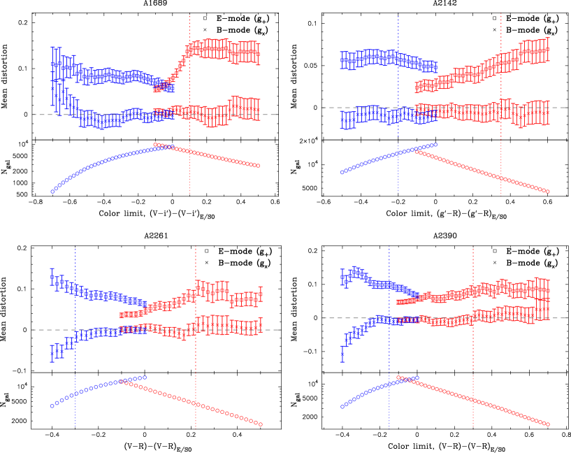
Figure 3.— Top panels: Mean shape distortions $(g_{+},g_{\times})$ averaged over the entire cluster region ($1^{\prime}<\theta<18^{\prime}$) for the four clusters done separately for the blue and red samples, in order to establish the boundaries of the color distribution free of cluster members. Bottom panels: Respective numbers of galaxies as a function of color-limit in the red (right) and the blue (blue) samples.

Figure 4.— Mass maps of the central $22^{\prime}\times 22^{\prime}$ of four AMiBA/Subaru clusters reconstructed from Subaru weak lensing data, with the gravitational shear field of background galaxies overlaid; $10\%$ ellipticity is indicated top right, and the resolution characterized by Gaussian FWHM is shown bottom right. Also overlaid are contours of the SZE flux densities at $94\,$GHz, observed with the 7-element AMiBA, given in units of $1\sigma$ reconstruction error. The resolution of AMiBA, given in Gaussian FWHM, is $6^{\prime}$ For all four clusters the distribution of the SZE signal is well correlated with the projected mass distribution, indicating that the hot gas in the clusters traces well the underlying gravitational potential dominated by unseen dark matter. The dark blue regions in the mass map of A2142 are outside the Subaru observations.

Figure 5.— Azimuthally-averaged radial profiles of the tangential reduced shear $g_{+}$ (upper panels) for the four clusters based on the combined red and blue background samples. The solid and dashed curves show the best-fitting NFW and SIS profiles for each cluster. Shown below is the $45^{\circ}$ rotated ($\times$) component, $g_{\times}$.

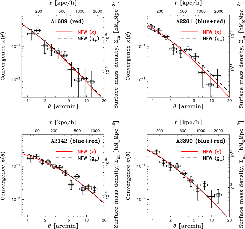
Figure 6.— Model-independent radial profiles of the lensing convergence $\kappa(\theta)=\Sigma_{m}(\theta)/\Sigma_{\rm crit}$ for the four clusters derived from a variant of the non-linear aperture-mass densitometry. For each cluster, the best-fitting NFW model for the $\kappa$ profile is shown with a solid line. The dashed curve shows the best-fitting NFW model for the $g_{+}$ profile in Figure 5.

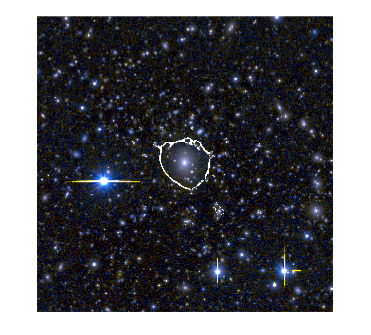
Figure 7.— Subaru $V+R_{\rm c}$ pseudo-color image of the central $6.7^{\prime}\times 6.7^{\prime}$ ($2{\rm K}\times 2{\rm K}$ pixels) region of the cluster A2261 at $z_{d}=0.226$. Overlaid is the tangential critical curve predicted for a background source at $z_{s}\sim 1.5$ based on strong lensing modeling of multiply-lensed images and tangential arcs registered in deep Subaru $VR_{\rm c}$ and CFHT/WIRCam $JHK_{S}$ images. The effective radius of the tangential critical curve defines the Einstein radius, $\theta_{\rm E}\approx 40^{\prime}$ at $z_{s}\sim 1.5$.

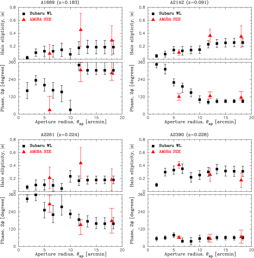
Figure 8.— Cluster ellipticity and orientation profiles on mass and ICM structure as a function of aperture radius $\theta_{\rm ap}$, measured from the Subaru weak lensing and AMiBA SZE maps shown in Figure 4. For each cluster, the top panel shows the halo ellipticity profile $|e^{\rm halo}|(\theta_{\rm ap})$, and the bottom panel shows the orientation profile $2\phi(\theta_{\rm ap})$, where $\phi^{\rm halo}$ represents the position angle of the major axis as measured from weighted quadrupole shape moments.

Figure 9.— Gas mass fraction profiles $\langle f_{\rm gas}(<r)\rangle=\langle M_{\rm gas}(<r)/M_{\rm tot}(<r)\rangle$ averaged over the sample of four hot ($T_{X}>8\,{\rm keV}$) clusters (A1689, A2142, A2261, A2390) obtained from joint AMiBA SZE and Subaru weak lensing observations, shown for the NFW-consistent Komatsu & Seljak 2001 model (black) and the isothermal $\beta$ model with $\beta=2/3$ (blue), along with published results (square, triangle, and circle) from other X-ray and SZE observations. The isothermal results exclude the cluster A2142 (see §6.4). For each model, the cross-hatched region represents $1\sigma$ uncertainties for the weighted mean at each radius point, including both the statistical measurement uncertainties and cluster-to-cluster variance. The black horizontal bar shows the constraints on the cosmic baryon fraction from the WMAP 5-year data.

Appendix A One-Dimensional Mass Reconstruction from Distortion Data

Following the method developed by Umetsu & Broadhurst (2008), we derive an expression for the discrete convergence profile using a non-linear extension of weak lensing aperture densitometry.

A.1. Non-Linear Aperture Mass Densitometry

For a shear-based estimation of the cluster mass profile we use a variant of weak lensing aperture densitometry, or the so-called $\zeta$-statistic (Fahlman et al., 1994; Clowe et al., 2000) of the form:

$$\zeta_{\rm c}(\theta) \equiv 2\int_{\theta}^{\theta_{\rm inn}}\!d\ln\theta^{\prime}\gamma_{+}(\theta^{\prime})$$ (A1)

$$+\frac{2}{1-(\theta_{\rm inn}/\theta_{\rm out})^{2}}\int_{\theta_{\rm inn}}^{\theta_{\rm out}}\!d\ln\theta^{\prime}\gamma_{+}(\theta^{\prime})$$

$$= \bar{\kappa}(\theta)-\bar{\kappa}(\theta_{\rm inn}<\vartheta<\theta_{\rm out}),$$

where $\kappa(\theta)$ is the azimuthal average of the convergence field $\kappa(\mbox{\boldmath$\theta$})$ at radius $\theta$, $\bar{\kappa}(\theta)$ is the average convergence interior to radius $\theta$, $\theta_{\rm inn}$ and $\theta_{\rm out}$ are the inner and outer radii of the annular background region in which the mean background contribution, $\bar{\kappa}_{b}\equiv\bar{\kappa}(\theta_{\rm inn}<\vartheta<\theta_{\rm out})$, is defined; $\gamma_{+}(\theta)=\bar{\kappa}(\theta)-\kappa(\theta)$ is an azimuthal average of the tangential component of the gravitational shear at radius $\theta$ (Fahlman et al., 1994), which is observable in the weak lensing limit: $\gamma_{+}(\theta)\approx\langle g_{+}(\theta)\rangle$. This cumulative mass estimator subtracts from the mean convergence $\bar{\kappa}(\theta)$ a constant $\bar{\kappa}_{b}$ for all apertures $\theta$ in the measurements, thus removing any DC component in the control region $\theta=[\theta_{\rm inn},\theta_{\rm out}]$. Note that the $\bar{\kappa}_{b}$ is a non-observable free parameter. This degree of freedom can be used to fix the outer boundary condition, and hence to derive a convergence profile $\kappa(\theta)$.

In the non-linear regime $\gamma_{+}(\theta)$ is not a direct observable. Therefore, non-linear corrections need to be taken into account in the mass reconstruction process (Umetsu & Broadhurst, 2008). In the subcritical regime (i.e., outside the critical curves), $\gamma_{+}(\theta)$ can be expressed in terms of the averaged tangential reduced shear as $\langle g_{+}(\theta)\rangle\approx\gamma_{+}(\theta)/[1-\kappa(\theta)]$ assuming a quasi-circular symmetry in the projected mass distribution (Broadhurst et al., 2005b; Umetsu et al., 2007). This non-linear equation (A1) for $\zeta_{\rm c}(\theta)$ can be solved by an iterative procedure: Since the weak lensing limit ($\kappa,|\gamma|,|g|\ll 1$) holds in the background region $\theta_{\rm inn}\leq\theta\leq\theta_{\rm max}$, we have the following iterative equation for $\zeta_{\rm c}(\theta)$:

$$\zeta_{\rm c}^{(k+1)}(\theta) \approx 2\int_{\theta}^{\theta_{\rm inn}}\!d\ln\theta^{\prime}\langle g_{+}(\theta)\rangle[1-\kappa^{(k)}(\theta)]$$ (A2)

$$+ \frac{2}{1-(\theta_{\rm inn}/\theta_{\rm out})^{2}}\int_{\theta_{\rm inn}}^{\theta_{\rm out}}\!d\ln\theta^{\prime}\langle g_{+}(\theta^{\prime})\rangle,$$

where $\zeta_{\rm c}^{(k+1)}$ represents the aperture densitometry in the $(k+1)$th step of the iteration $(k=0,1,2,...,N_{\rm iter})$; the $\kappa^{(k+1)}$ is calculated from $\zeta_{\rm c}^{(k+1)}$ using equation (A10). This iteration is preformed by starting with $\kappa^{(0)}=0$ for all radial bins, and repeated until convergence is reached at all radial bins. For a fractional tolerance of $1\times 10^{-5}$, this iteration procedure converges within $N_{\rm iter}\sim 10$ iterations. We compute errors for $\zeta_{\rm c}$ and $\kappa$ with the linear approximation.

A.2. Discretized Estimator for the Lensing Convergence

In the continuous limit, the averaged convergence $\bar{\kappa}(\theta)$ and the convergence $\kappa(\theta)$ are related by

$$\bar{\kappa}(\theta) = \frac{2}{\theta^{2}}\int_{0}^{\theta}\!d\ln\theta^{\prime}\theta^{\prime 2}\kappa(\theta^{\prime}),$$ (A3)

$$\kappa(\theta) = \frac{1}{2\theta^{2}}\frac{d(\theta^{2}\bar{\kappa})}{d\ln\theta}.$$ (A4)

For a given set of annular radii $\theta_{m}$ $(m=1,2,...,N)$, discretized estimators can be written in the following way:

$$\bar{\kappa}_{m} \equiv \bar{\kappa}(\theta_{m})=\frac{2}{\theta_{m}^{2}}\sum_{l=1}^{m-1}\Delta\ln\theta_{l}\bar{\theta}_{l}^{2}\kappa(\bar{\theta}_{l}),$$ (A5)

$$\kappa_{l} \equiv \kappa(\bar{\theta}_{l})=\alpha^{l}_{2}\bar{\kappa}_{l+1}-\alpha^{l}_{1}\bar{\kappa}_{l}\ \ \ \ \ (l=1,2,...,N-1),$$ (A6)

where

$$\alpha_{1}^{l}=\frac{1}{2\Delta\ln\theta_{l}}\left(\frac{\theta_{l}}{\overline{\theta}_{l}}\right)^{2},\,\,\alpha_{2}^{l}=\frac{1}{2\Delta\ln\theta_{l}}\left(\frac{\theta_{l+1}}{\overline{\theta}_{l}}\right)^{2},$$ (A7)

with $\Delta\ln\theta_{l}\equiv(\theta_{l+1}-\theta_{l})/\bar{\theta}_{l}$ and $\bar{\theta}_{l}$ being the area-weighted center of the $l$th annulus defined by $\theta_{l}$ and $\theta_{l+1}$; in the continuous limit, we have

$$\bar{\theta}_{l} \equiv 2\int_{\theta_{l}}^{\theta_{l+1}}\!d\theta^{\prime}\theta^{\prime 2}/(\theta_{l+1}^{2}-\theta_{l}^{2})$$ (A8)

$$= \frac{2}{3}\frac{\theta_{l}^{2}+\theta_{l+1}^{2}+\theta_{l}\theta_{l+1}}{\theta_{l}+\theta_{l+1}}.$$

The technique of the aperture densitometry allows us to measure the azimuthally averaged convergence $\bar{\kappa}(\theta)$ up to an additive constant $\bar{\kappa}_{b}$, corresponding to the mean convergence in the outer background annulus with inner and outer radii of $\theta_{\rm inn}$ and $\theta_{\rm out}$, respectively:

$$\bar{\kappa}(\theta)=\zeta_{\rm c}(\theta)+\bar{\kappa}_{b}.$$ (A9)

Substituting equation (A9) into equation (A6) yields the desired expression as

$$\kappa(\theta_{l})=\alpha^{l}_{2}\zeta_{\rm c}(\theta_{l+1})-\alpha^{l}_{1}\zeta_{\rm c}(\theta_{l})+(\alpha_{2}^{l}-\alpha_{1}^{l})\bar{\kappa}_{b}.$$ (A10)

Finally, the error covariance matrix of $\kappa_{l}$ is expressed as

$$C_{kl}\equiv\langle\delta\kappa_{k}\delta\kappa_{l}\rangle = \alpha_{2}^{k}\alpha_{2}^{l}C^{\zeta}_{k+1,l+1}+\alpha_{1}^{k}\alpha_{1}^{l}C^{\zeta}_{k,l}$$ (A11)

$$- \alpha_{1}^{k}\alpha_{2}^{l}C^{\zeta}_{k,l+1}-\alpha_{2}^{k}\alpha_{1}^{l}C^{\zeta}_{k+1,l},$$

where $C^{\zeta}_{kl}\equiv\langle\delta\zeta_{k}\delta\zeta_{l}\rangle$ is the bin-to-bin error covariance matrix of the aperture densitometry measurements which is calculated by propagating the rms errors $\sigma_{+}(\theta_{l})$ for the tangential shear measurement.

References

- Afshordi et al. (2007) Afshordi, N., Lin, Y.-T., Nagai, D., & Sanderson, A. J. R. 2007, MNRAS, 378, 293
- Allen et al. (2001) Allen, S. W., Ettori, S., & Fabian, A. C. 2001, MNRAS, 324, 877
- Allen et al. (2008) Allen, S. W., Rapetti, D. A., Schmidt, R. W., Ebeling, H., Morris, R. G., & Fabian, A. C. 2008, MNRAS, 383, 879
- Allen et al. (2004) Allen, S. W., Schmidt, R. W., Ebeling, H., Fabian, A. C., & van Speybroeck, L. 2004, MNRAS, 353, 457
- Allen et al. (2002) Allen, S. W., Schmidt, R. W., & Fabian, A. C. 2002, MNRAS, 334, L11
- Atrio-Barandela et al. (2008) Atrio-Barandela, F., Kashlinsky, A., Kocevski, D., & Ebeling, H. 2008, ApJ, 675, L57
- Bartelmann (1996) Bartelmann, M. 1996, A&A, 313, 697
- Bartelmann et al. (1996) Bartelmann, M., Narayan, R., Seitz, S., & Schneider, P. 1996, ApJ, 464, L115+
- Bartelmann & Schneider (2001) Bartelmann, M., & Schneider, P. 2001, Phys. Rep., 340, 291
- Benson et al. (2004) Benson, B. A., Church, S. E., Ade, P. A. R., Bock, J. J., Ganga, K. M., Henson, C. N., & Thompson, K. L. 2004, ApJ, 617, 829
- Bertin & Arnouts (1996) Bertin, E., & Arnouts, S. 1996, A&AS, 117, 393
- Bialek et al. (2001) Bialek, J. J., Evrard, A. E., & Mohr, J. J. 2001, ApJ, 555, 597
- Birkinshaw (1999) Birkinshaw, M. 1999, Phys. Rep., 310, 97
- Boehringer et al. (1998) Boehringer, H., Tanaka, Y., Mushotzky, R. F., Ikebe, Y., & Hattori, M. 1998, A&A, 334, 789
- Broadhurst et al. (2005a) Broadhurst, T., Benítez, N., Coe, D., Sharon, K., Zekser, K., White, R., Ford, H., Bouwens, R., Blakeslee, J., Clampin, M., Cross, N., Franx, M., Frye, B., Hartig, G., Illingworth, G., Infante, L., Menanteau, F., Meurer, G., Postman, M., Ardila, D. R., Bartko, F., Brown, R. A., Burrows, C. J., Cheng, E. S., Feldman, P. D., Golimowski, D. A., Goto, T., Gronwall, C., Herranz, D., Holden, B., Homeier, N., Krist, J. E., Lesser, M. P., Martel, A. R., Miley, G. K., Rosati, P., Sirianni, M., Sparks, W. B., Steindling, S., Tran, H. D., Tsvetanov, Z. I., & Zheng, W. 2005a, ApJ, 621, 53
- Broadhurst et al. (2005b) Broadhurst, T., Takada, M., Umetsu, K., Kong, X., Arimoto, N., Chiba, M., & Futamase, T. 2005b, ApJ, 619, L143
- Broadhurst et al. (2008) Broadhurst, T., Umetsu, K., Medezinski, E., Oguri, M., & Rephaeli, Y. 2008, ApJ, 685, L9
- Biviano & Salucci (2006) Biviano, A. & Salucci, P. 2006, A&A, 452, 75
- Bullock et al. (2001) Bullock, J. S., Kolatt, T. S., Sigad, Y., Somerville, R. S., Kravtsov, A. V., Klypin, A. A., Primack, J. R., & Dekel, A. 2001, MNRAS, 321, 559
- Capak et al. (2007) Capak, P., Aussel, H., Ajiki, M., McCracken, H. J., Mobasher, B., Scoville, N., Shopbell, P., Taniguchi, Y., Thompson, D., Tribiano, S., Sasaki, S., Blain, A. W., Brusa, M., Carilli, C., Comastri, A., Carollo, C. M., Cassata, P., Colbert, J., Ellis, R. S., Elvis, M., Giavalisco, M., Green, W., Guzzo, L., Hasinger, G., Ilbert, O., Impey, C., Jahnke, K., Kartaltepe, J., Kneib, J.-P., Koda, J., Koekemoer, A., Komiyama, Y., Leauthaud, A., Lefevre, O., Lilly, S., Liu, C., Massey, R., Miyazaki, S., Murayama, T., Nagao, T., Peacock, J. A., Pickles, A., Porciani, C., Renzini, A., Rhodes, J., Rich, M., Salvato, M., Sanders, D. B., Scarlata, C., Schiminovich, D., Schinnerer, E., Scodeggio, M., Sheth, K., Shioya, Y., Tasca, L. A. M., Taylor, J. E., Yan, L., & Zamorani, G. 2007, ApJS, 172, 99
- Capak et al. (2004) Capak, P., Cowie, L. L., Hu, E. M., Barger, A. J., Dickinson, M., Fernandez, E., Giavalisco, M., Komiyama, Y., Kretchmer, C., McNally, C., Miyazaki, S., Okamura, S., & Stern, D. 2004, AJ, 127, 180
- Carlstrom et al. (2002) Carlstrom, J. E., Holder, G. P., & Reese, E. D. 2002, ARA&A, 40, 643
- Challinor & Lasenby (1998) Challinor, A., & Lasenby, A. 1998, ApJ, 499, 1
- Chen et al. (2008) Chen, M.-T et al.. 2008, ApJ, submitted
- Clowe et al. (2006) Clowe, D., Bradač, M., Gonzalez, A. H., Markevitch, M., Randall, S. W., Jones, C., & Zaritsky, D. 2006, ApJ, 648, L109
- Clowe et al. (2000) Clowe, D., Luppino, G. A., Kaiser, N., & Gioia, I. M. 2000, ApJ, 539, 540
- Corless & King (2007) Corless, V. L., & King, L. J. 2007, MNRAS, 380, 149
- Crain et al. (2007) Crain, R. A., Eke, V. R., Frenk, C. S., Jenkins, A., McCarthy, I. G., Navarro, J. F., & Pearce, F. R. 2007, MNRAS, 377, 41
- Crittenden et al. (2002) Crittenden, R. G., Natarajan, P., Pen, U.-L., & Theuns, T. 2002, ApJ, 568, 20
- Duffy et al. (2008) Duffy, A. R., Schaye, J., Kay, S. T., & Dalla Vecchia, C. 2008, MNRAS, 390, L64
- Dunkley et al. (2008) Dunkley, J., Komatsu, E., Nolta, M. R., Spergel, D. N., Larson, D., Hinshaw, G., Page, L., Bennett, C. L., Gold, B., Jarosik, N., Weiland, J. L., Halpern, M., Hill, R. S., Kogut, A., Limon, M., Meyer, S. S., Tucker, G. S., Wollack, E., & Wright, E. L. 2008, ApJS, submitted (arXiv:0803.0586)
- Erben et al. (2001) Erben, T., Van Waerbeke, L., Bertin, E., Mellier, Y., & Schneider, P. 2001, A&A, 366, 717
- Fahlman et al. (1994) Fahlman, G., Kaiser, N., Squires, G., & Woods, D. 1994, ApJ, 437, 56
- Frye & Broadhurst (1998) Frye, B., & Broadhurst, T. 1998, ApJ, 499, L115+
- Fukugita et al. (1998) Fukugita, M., Hogan, C. J., & Peebles, P. J. E. 1998, ApJ, 503, 518
- Gavazzi et al. (2003) Gavazzi, R., Fort, B., Mellier, Y., Pelló, R., & Dantel-Fort, M. 2003, A&A, 403, 11
- Gonzalez et al. (2005) Gonzalez, A. H., Zabludoff, A. I., & Zaritsky, D. 2005, ApJ, 618, 195
- Grego et al. (2001a) Grego, L., Carlstrom, J. E., Reese, E. D., Holder, G. P., Holzapfel, W. L., Joy, M. K., Mohr, J. J., & Patel, S. 2001a, ApJ, 552, 2
- Grego et al. (2001b) —. 2001b, ApJ, 552, 2
- Halkola et al. (2006) Halkola, A., Seitz, S., & Pannella, M. 2006, MNRAS, 372, 1425
- Halverson et al. (2008) Halverson, N. W., Lanting, T., Ade, P. A. R., Basu, K., Bender, A. N., Benson, B. A., Bertoldi, F., Cho, H. ., Chon, G., Clarke, J., Dobbs, M., Ferrusca, D., Guesten, R., Holzapfel, W. L., Kovacs, A., Kennedy, J., Kermish, Z., Kneissl, R., Lee, A. T., Lueker, M., Mehl, J., Menten, K. M., Muders, D., Nord, M., Pacaud, F., Plagge, T., Reichardt, C., Richards, P. L., Schaaf, R., Schilke, P., Schuller, F., Schwan, D., Spieler, H., Tucker, C., Weiss, A., & Zahn, O. 2008, ApJ, submitted (arXiv:0807.4208)
- Hamana et al. (2003) Hamana, T., Miyazaki, S., Shimasaku, K., Furusawa, H., Doi, M., Hamabe, M., Imi, K., Kimura, M., Komiyama, Y., Nakata, F., Okada, N., Okamura, S., Ouchi, M., Sekiguchi, M., Yagi, M., & Yasuda, N. 2003, ApJ, 597, 98
- Hattori et al. (1999) Hattori, M., Kneib, J., & Makino, N. 1999, Progress of Theoretical Physics Supplement, 133, 1
- Hennawi et al. (2007) Hennawi, J. F., Dalal, N., Bode, P., & Ostriker, J. P. 2007, ApJ, 654, 714
- Heymans et al. (2006) Heymans, C., Van Waerbeke, L., Bacon, D., Berge, J., Bernstein, G., Bertin, E., Bridle, S., Brown, M. L., Clowe, D., Dahle, H., Erben, T., Gray, M., Hetterscheidt, M., Hoekstra, H., Hudelot, P., Jarvis, M., Kuijken, K., Margoniner, V., Massey, R., Mellier, Y., Nakajima, R., Refregier, A., Rhodes, J., Schrabback, T., & Wittman, D. 2006, MNRAS, 368, 1323
- Ho et al. (2008) Ho, P. T. P. et al. 2008, ApJ, submitted (arXiv:0810.1871)
- Hoekstra et al. (1998) Hoekstra, H., Franx, M., Kuijken, K., & Squires, G. 1998, ApJ, 504, 636
- Huang et al. (2008) Huang, C.-W. L. et al. 2008, in preparation
- Itoh et al. (1998) Itoh, N., Kohyama, Y., & Nozawa, S. 1998, ApJ, 502, 7
- Jain et al. (2000) Jain, B., Seljak, U., & White, S. 2000, ApJ, 530, 547
- Jing & Suto (2002) Jing, Y. P., & Suto, Y. 2002, ApJ, 574, 538
- Kaiser (1995) Kaiser, N. 1995, ApJ, 439, L1
- Kaiser & Squires (1993) Kaiser, N., & Squires, G. 1993, ApJ, 404, 441
- Kaiser et al. (1995) Kaiser, N., Squires, G., & Broadhurst, T. 1995, ApJ, 449, 460
- Kawahara et al. (2007) Kawahara, H., Suto, Y., Kitayama, T., Sasaki, S., Shimizu, M., Rasia, E., & Dolag, K. 2007, ApJ, 659, 257
- Kneib et al. (2003) Kneib, J.-P., Hudelot, P., Ellis, R. S., Treu, T., Smith, G. P., Marshall, P., Czoske, O., Smail, I., & Natarajan, P. 2003, ApJ, 598, 804
- Kneissl et al. (2001) Kneissl, R., Jones, M. E., Saunders, R., Eke, V. R., Lasenby, A. N., Grainge, K., & Cotter, G. 2001, MNRAS, 328, 783
- Koch et al. (2008a) Koch, P. et al. 2008a, ApJS, submitted
- Koch et al. (2008b) —. 2008b, in preparation
- Koch et al. (2006) Koch, P., Raffin, P. A., Proty Wu, J.-H., & et al. 2006, in ESA Special Publication, Vol. 626, The European Conference on Antennas and Propagation: EuCAP 2006
- Komatsu et al. (2008) Komatsu, E., Dunkley, J., Nolta, M. R., Bennett, C. L., Gold, B., Hinshaw, G., Jarosik, N., Larson, D., Limon, M., Page, L., Spergel, D. N., Halpern, M., Hill, R. S., Kogut, A., Meyer, S. S., Tucker, G. S., Weiland, J. L., Wollack, E., & Wright, E. L. 2008, ApJS, submitted (arXiv:0803.0547)
- Komatsu & Seljak (2001) Komatsu, E., & Seljak, U. 2001, MNRAS, 327, 1353
- Komatsu & Seljak (2002) —. 2002, MNRAS, 336, 1256
- Kravtsov et al. (2005) Kravtsov, A. V., Nagai, D., & Vikhlinin, A. A. 2005, ApJ, 625, 588
- Lancaster et al. (2005) Lancaster, K., Genova-Santos, R., Falcòn, N., Grainge, K., Gutièrrez, C., Kneissl, R., Marshall, P., Pooley, G., Rebolo, R., Rubiño-Martin, J.-A., Saunders, R. D. E., Waldram, E., & Watson, R. A. 2005, MNRAS, 359, 16
- Lemze et al. (2008a) Lemze, D., Barkana, R., Broadhurst, T. J., & Rephaeli, Y. 2008a, MNRAS, 386, 1092
- Lemze et al. (2008b) Lemze, D., Broadhurst, T., Rephaeli, Y., Barkana, R., Czoske, O., & Umetsu, K. 2008b, submitted to ApJ (arXiv:0810.3129)
- Limousin et al. (2007) Limousin, M., Richard, J., Jullo, E., Kneib, J.-P., Fort, B., Soucail, G., Elíasdóttir, Á., Natarajan, P., Ellis, R. S., Smail, I., Czoske, O., Smith, G. P., Hudelot, P., Bardeau, S., Ebeling, H., Egami, E., & Knudsen, K. K. 2007, ApJ, 668, 643
- Lin et al. (2008) Lin, K.-Y. et al., ApJ, submitted
- Liu et al. (2008) Liu, G.-C. et al., in preparation
- Mandelbaum et al. (2008) Mandelbaum, R., Seljak, U., & Hirata, C. M. 2008, Journal of Cosmology and Astro-Particle Physics, 8, 6
- Markevitch (1998) Markevitch, M. 1998, ApJ, 504, 27
- Markevitch et al. (1998) Markevitch, M., Forman, W. R., Sarazin, C. L., & Vikhlinin, A. 1998, ApJ, 503, 77
- Markevitch et al. (2002) Markevitch, M., Gonzalez, A. H., David, L., Vikhlinin, A., Murray, S., Forman, W., Jones, C., & Tucker, W. 2002, ApJ, 567, L27
- Markevitch et al. (2000) Markevitch, M., Ponman, T. J., Nulsen, P. E. J., Bautz, M. W., Burke, D. J., David, L. P., Davis, D., Donnelly, R. H., Forman, W. R., Jones, C., Kaastra, J., Kellogg, E., Kim, D.-W., Kolodziejczak, J., Mazzotta, P., Pagliaro, A., Patel, S., Van Speybroeck, L., Vikhlinin, A., Vrtilek, J., Wise, M., & Zhao, P. 2000, ApJ, 541, 542
- Mason et al. (2001) Mason, B. S., Myers, S. T., & Readhead, A. C. S. 2001, ApJ, 555, L11
- Mason et al. (2003) Mason, B. S., Pearson, T. J., Readhead, A. C. S., Shepherd, M. C., Sievers, J., Udomprasert, P. S., Cartwright, J. K., Farmer, A. J., Padin, S., Myers, S. T., Bond, J. R., Contaldi, C. R., Pen, U., Prunet, S., Pogosyan, D., Carlstrom, J. E., Kovac, J., Leitch, E. M., Pryke, C., Halverson, N. W., Holzapfel, W. L., Altamirano, P., Bronfman, L., Casassus, S., May, J., & Joy, M. 2003, ApJ, 591, 540
- Maughan et al. (2008) Maughan, B. J., Jones, C., Forman, W., & Van Speybroeck, L. 2008, ApJS, 174, 117
- Mazzotta et al. (2004) Mazzotta, P., Rasia, E., Moscardini, L., & Tormen, G. 2004, MNRAS, 354, 10
- Medezinski et al. (2007) Medezinski, E., Broadhurst, T., Umetsu, K., Coe, D., Benítez, N., Ford, H., Rephaeli, Y., Arimoto, N., & Kong, X. 2007, ApJ, 663, 717
- Miyazaki et al. (2002) Miyazaki, S., Komiyama, Y., Sekiguchi, M., Okamura, S., Doi, M., Furusawa, H., Hamabe, M., Imi, K., Kimura, M., Nakata, F., Okada, N., Ouchi, M., Shimasaku, K., Yagi, M., & Yasuda, N. 2002, PASJ, 54, 833
- Molnar et al. (2008) Molnar, S. M. et al. 2008, in preparation
- Mroczkowski et al. (2008) Mroczkowski, T., Bonamente, M., Carlstrom, J. E., Culverhouse, T. L., Greer, C., Hawkins, D., Hennessy, R., Joy, M., Lamb, J. W., Leitch, E. M., Loh, M., Maughan, B., Marrone, D. P., Miller, A., Nagai, D., Muchovej, S., Pryke, C., Sharp, M., & Woody, D. 2008, ApJ, submitted (arXiv:0809.5077)
- Myers et al. (1997) Myers, S. T., Baker, J. E., Readhead, A. C. S., Leitch, E. M., & Herbig, T. 1997, ApJ, 485, 1
- Navarro et al. (1996) Navarro, J. F., Frenk, C. S., & White, S. D. M. 1996, ApJ, 462, 563
- Navarro et al. (1997) —. 1997, ApJ, 490, 493
- Neto et al. (2007) Neto, A. F., Gao, L., Bett, P., Cole, S., Navarro, J. F., Frenk, C. S., White, S. D. M., Springel, V., & Jenkins, A. 2007, MNRAS, 381, 1450
- Nishioka et al. (2008) Nishioka, H. et al. 2008, ApJ, accepted (arXiv:0811.1675)
- Oguri & Blandford (2008) Oguri, M., & Blandford, R. D. 2008, preprint (arXiv:0808.0192O)
- Oguri et al. (2005) Oguri, M., Takada, M., Umetsu, K., & Broadhurst, T. 2005, ApJ, 632, 841
- Okabe & Umetsu (2008) Okabe, N., & Umetsu, K. 2008, PASJ, 60, 345
- Padin et al. (2001) Padin, S., Cartwright, J. K., Mason, B. S., Pearson, T. J., Readhead, A. C. S., Shepherd, M. C., Sievers, J., Udomprasert, P. S., Holzapfel, W. L., Myers, S. T., Carlstrom, J. E., Leitch, E. M., Joy, M., Bronfman, L., & May, J. 2001, ApJ, 549, L1
- Padin et al. (2002) Padin, S., Shepherd, M. C., Cartwright, J. K., Keeney, R. G., Mason, B. S., Pearson, T. J., Readhead, A. C. S., Schaal, W. A., Sievers, J., Udomprasert, P. S., Yamasaki, J. K., Holzapfel, W. L., Carlstrom, J. E., Joy, M., Myers, S. T., & Otarola, A. 2002, PASP, 114, 83
- Pearson et al. (2003) Pearson, T. J., Mason, B. S., Readhead, A. C. S., Shepherd, M. C., Sievers, J. L., Udomprasert, P. S., Cartwright, J. K., Farmer, A. J., Padin, S., Myers, S. T., Bond, J. R., Contaldi, C. R., Pen, U.-L., Prunet, S., Pogosyan, D., Carlstrom, J. E., Kovac, J., Leitch, E. M., Pryke, C., Halverson, N. W., Holzapfel, W. L., Altamirano, P., Bronfman, L., Casassus, S., May, J., & Joy, M. 2003, ApJ, 591, 556
- Press et al. (1992) Press, W. H., Teukolsky, S. A., Vetterling, W. T., Flannery, B. P., 1992, Numerical Recipes in FORTRAN: The Art of Scientific Computing, Third Edition, Cambridge University Press.
- Reese et al. (2002) Reese, E. D., Carlstrom, J. E., Joy, M., Mohr, J. J., Grego, L., & Holzapfel, W. L. 2002, ApJ, 581, 53
- Rephaeli (1995) Rephaeli, Y. 1995, ARA&A, 33, 541
- Rines & Geller (2008) Rines, K., & Geller, M. J. 2008, AJ, 135, 1837
- Sanderson et al. (2003) Sanderson, A. J. R., Ponman, T. J., Finoguenov, A., Lloyd-Davies, E. J., & Markevitch, M. 2003, MNRAS, 340, 989
- Sasaki (1996) Sasaki, S. 1996, PASJ, 48, L119
- Saxton & Wu (2008) Saxton, C. J., & Wu, K. 2008, MNRASin press (arXiv:0809.3795)
- Schneider & Seitz (1995) Schneider, P., & Seitz, C. 1995, A&A, 294, 411
- Sereno (2007) Sereno, M. 2007, MNRAS, 380, 1207
- Spergel et al. (2007) Spergel, D. N., Bean, R., Doré, O., Nolta, M. R., Bennett, C. L., Dunkley, J., Hinshaw, G., Jarosik, N., Komatsu, E., Page, L., Peiris, H. V., Verde, L., Halpern, M., Hill, R. S., Kogut, A., Limon, M., Meyer, S. S., Odegard, N., Tucker, G. S., Weiland, J. L., Wollack, E., & Wright, E. L. 2007, ApJS, 170, 377
- Umetsu & Broadhurst (2008) Umetsu, K., & Broadhurst, T. 2008, ApJ, 684, 177
- Umetsu et al. (2004) Umetsu, K., Chiueh, T., Lin, K.-Y., Wu, J.-M., & Tseng, Y.-H. 2004, Modern Physics Letters A, 19, 1027
- Umetsu et al. (1999) Umetsu, K., Tada, M., & Futamase, T. 1999, Progress of Theoretical Physics Supplement, 133, 53
- Umetsu et al. (2007) Umetsu, K., Takada, M., & Broadhurst, T. 2007, Modern Physics Letters A, 22, 2099
- Umetsu et al. (2005) Umetsu, K., Wu, J.-M., Chiueh, T., & Birkinshaw, M. 2005, preprint (arXiv:astro-ph/0607542)
- Vikhlinin et al. (2006) Vikhlinin, A., Kravtsov, A., Forman, W., Jones, C., Markevitch, M., Murray, S. S., & Van Speybroeck, L. 2006, ApJ, 640, 691
- Watson et al. (2003) Watson, R. A., Carreira, P., Cleary, K., Davies, R. D., Davis, R. J., Dickinson, C., Grainge, K., Gutiérrez, C. M., Hobson, M. P., Jones, M. E., Kneissl, R., Lasenby, A., Maisinger, K., Pooley, G. G., Rebolo, R., Rubiño-Martin, J. A., Rusholme, B., Saunders, R. D. E., Savage, R., Scott, P. F., Slosar, A., Sosa Molina, P. J., Taylor, A. C., Titterington, D., Waldram, E., & Wilkinson, A. 2003, MNRAS, 341, 1057
- Worrall & Birkinshaw (2006) Worrall, D. M., & Birkinshaw, M. 2006, in Lecture Notes in Physics, Berlin Springer Verlag, Vol. 693, Physics of Active Galactic Nuclei at all Scales, ed. D. Alloin, 39–+
- Wright & Brainerd (2000) Wright, C. O., & Brainerd, T. G. 2000, ApJ, 534, 34
- Wu et al. (2008a) Wu, J. H. P. et al. 2008, ApJ, submitted (arXiv:0810.1015)
- Wu et al. (2008b) Wu, J.-H. P., Chiueh, T.-H., Huang, C.-W., Liao, Y.-W., Wang, F.-C., Altimirano, P., Chang, C.-H., Chang, S.-H., Chang, S.-W., Chen, M.-T., Chereau, G., Han, C.-C., Ho, P. T. P., Huang, Y.-D., Hwang, Y.-J., Jiang, H., Koch, P., Kubo, D., Li, C.-T., Lin, K.-Y., Liu, G.-C., Martin-Cocher, P., Molnar, S., Nishioka, H., Raffin, P., Umetsu, K., Kesteven, M., Wilson, W., Birkinshaw, M., & Lancaster, K. 2008b, Modern Physics Letters A, 23, 1675
- Yagi et al. (2002) Yagi, M., Kashikawa, N., Sekiguchi, M., Doi, M., Yasuda, N., Shimasaku, K., & Okamura, S. 2002, AJ, 123, 66
- Yoshikawa et al. (2000) Yoshikawa, K., Jing, Y. P., & Suto, Y. 2000, ApJ, 535, 593
- Zhang et al. (2002) Zhang, P., Pen, U.-L., & Wang, B. 2002, ApJ, 577, 555