IRAM-PdBI Observations of Binary Protostars I: The Hierarchical System SVS 13 in NGC 1333

Abstract

We present millimeter interferometric observations of the young stellar object SVS 13 in NCG 1333 in the N₂H⁺ (1–0) line and at 1.4 and 3 mm dust continuum, using the IRAM Plateau de Bure interferometer. The results are complemented by infrared data from the Spitzer Space Telescope. The millimeter dust continuum images resolve four sources (A, B, C, and VLA 3) in SVS 13. With the dust continuum images, we derive gas masses of 0.2 $-$ 1.1 $M_{\odot}$ for the sources. N₂H⁺ (1–0) line emission is detected and spatially associated with the dust continuum sources B and VLA 3. The observed mean line width is $\sim$ 0.48 km s^-1 and the estimated virial mass is $\sim$ 0.7 $M_{\odot}$. By simultaneously fitting the seven hyperfine line components of N₂H⁺, we derive the velocity field and find a symmetric velocity gradient of $\sim$ 28 km s^-1 pc^-1 across sources B and VLA 3, which could be explained by core rotation. The velocity field suggests that sources B and VLA 3 are forming a physically bound protobinary system embedded in a common N₂H⁺ core. $Spitzer$ images show mid-infrared emission from sources A and C, which is spatially associated with the mm dust continuum emission. No infrared emission is detected from source B, implying that the source is deeply embedded. Based on the morphologies and velocity structure, we propose a hierarchical fragmentation picture for SVS 13 where the three sources (A, B, and C) were formed by initial fragmentation of a filamentary prestellar core, while the protobinary system (sources B and VLA 3) was formed by rotational fragmentation of a single collapsing sub-core.

1 INTRODUCTION

Although both observations and theoretical simulations support the hypothesis that the fragmentation of collapsing protostellar cores is the main mechanism for the formation of binary/multiple stellar systems, many key questions concerning this fragmentation process, e.g., the exact when, where, why, and how, are still under debate (see reviews by Bodenheimer et al. 2000, Tohline 2002, and Goodwin et al. 2007). To answer these questions, direct observations of the earliest, embedded phase of binary star formation are needed to study in detail their kinematics. This was unfortunately long hampered by the low angular resolution of millimeter (mm) telescopes. However, the recent availability of large millimeter interferometers has enabled us to directly observe the formation phase of binary stars, although the number of known and well-studied systems is still very small (see Launhardt 2004).

To search for binary protostars and to derive their kinematic properties, we have started a systematic program to observe, at high angular resolution, a number of isolated low-mass (pre-) protostellar molecular cloud cores. The initial survey was conducted at the Owens Valley Radio Observatory (OVRO) millimeter-wave array (Launhardt 2004; Chen et al. 2007, hereafter Paper I; Launhardt et al. in prep.), and is now continued with the Australia Telescope Compact Array (ATCA; Chen et al. 2008a, hereafter Paper II), the Submillimeter Array (SMA; Chen et al. 2008b), and the IRAM Plateau de Bure Interferometer (PdBI) array (this work and Chen et al. in prep.).

SVS 13 is a young stellar object (YSO) located in the NGC 1333 star-forming region at a distance of 350 pc (Herbig & Jones 1983). It was discovered as a near-infrared (NIR) source by Strom et al. (1976). At least three mm continuum sources were detected around SVS 13 (Chini et al. 1997; Bachiller et al. 1998, hereafter B98) and named A, B, and C, respectively (Looney et al. 2000, hereafter LMW2000). Source A is coincident with the infrared/optical source SVS 13, source B is located $\sim$ 15^′′ southwest of A, and source C is further to the southwest (B98; LMW2000). With BIMA observations, LMW2000 detected another mm source located $\sim$ 6^′′ southwest of source A, which is coincident with the radio source VLA 3 in the VLA survey of this region (Rodríguez et al. 1997; 1999). More recently, Anglada et al. (2000; 2004) revealed that source A is actually a binary system with an angular separation of 0$\farcs$3. Located to the southeast of SVS 13 is the well-known chain of Herbig-Haro (HH) objects 7$-$11 (Herbig 1974; Strom et al. 1974; Khanzadyan et al. 2003 and references therein). Although several possible driving candidates have been proposed for this large-scale HH chain (e.g., Rodríguez et al. 1997), high-resolution CO (2–1) observations (Bachiller et al. 2000, hereafter B2000), as well as an analysis of the spectral energy distributions (LMW2000), clearly favor SVS13 A as the driving source. In this paper, we present our IRAM-PdBI observations in the N₂H⁺ (1–0) line and at the 1.4 and 3 mm dust continuum toward SVS 13, together with complementary infrared data from the Spitzer Space Telescope (hereafter $Spitzer$). In Section 2 we describe the observations and data reduction; Observational results are presented in Section 3 and discussed in Section 4; The main conclusions of this study are summarized in Section 5.

2 OBSERVATIONS AND DATA REDUCTION

2.1 IRAM PdBI Observations

Millimeter interferometric observations of SVS 13 were carried out with the IRAM PdBI in 2006 March (C configuration with 6 antennas) and July (D configuration with 5 antennas). The 3 mm and 1 mm bands were observed simultaneously, with baselines ranging from 16 m to 176 m. During the observations, two receivers were tuned to the N₂H⁺ (1–0) line at 93.1378 GHz and the ¹³CO (2–1) line at 220 GHz, respectively. Bandwidths in the N₂H⁺ line and ¹³CO line were 20 MHz and 40 MHz, resulting in channel spacings of 39 kHz and 79 kHz and velocity resolutions of 0.2 km s^-1 and 0.1 km s^-1, respectively. The remaining windows of the correlator were combined to observe the dust continuum emission with a total band width of 500 MHz at both $\lambda$ 3 mm and $\lambda$ 1.4 mm. System temperatures of the 3 mm and 1 mm receivers were typically 110 $-$ 200 K and $\sim$ 300 K, respectively. The (naturally-weighted) synthesized half-power beam widths were 2$\farcs$8 $\times$ 2$\farcs$5 at 93.2 GHz and 1$\farcs$2 $\times$ 1$\farcs$1 at 220 GHz. The FWHM primary beams were $\sim$ 54^′′ and 23^′′, respectively. Several nearby phase calibrators were observed to determine the time-dependent complex antenna gains. The correlator bandpass was calibrated with the sources 3C273 and 1749+096, while the absolute flux density scale was derived from 3C345. The flux calibration uncertainty was estimated to be $\sim$ 15%. Only N₂H⁺ line data were used here because the signal-to-noise ratio of the ¹³CO line data was much lower in the 3 mm observational conditions, although the quality of the 1.4 mm dust continuum data is sufficient for our science goals. The data were calibrated and reduced using the GILDAS software. Observing parameters are summarized in Table 1.

2.2 Spitzer Observations

Mid-infrared data were obtained from the $Spitzer$ Science Center. SVS 13 was observed by $Spitzer$ on 2004 September 8th with the Infrared Array Camera (IRAC; AOR key 5793280) and September 20th with the Multiband Imaging Photometer for $Spitzer$ (MIPS; AOR key 5789440). The source was observed as part of the c2d Legacy program (Evans et al. 2003). The data were processed by the $Spitzer$ Science Center using their standard pipeline (version S14.0) to produce Post Basic Calibrated Data (P-BCD) images, which are flux-calibrated into physical units (MJy sr^-1). Further analysis and figures were completed with the IRAF and GILDAS software packages.

3 RESULTS

3.1 IRAM-PdBI Results

3.1.1 Millimeter Dust Continuum Emission

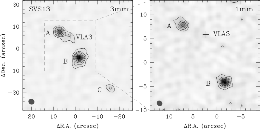
Figure 1: IRAM-PdBI mm dust continuum images of SVS 13. Contours start at $\sim$ 3 $\sigma$ (see Table 1) by steps of $\sim$ 2 $\sigma$. Crosses in the images mark the position of the radio source VLA 3 (Rodríguez et al. 1997). The synthesized PdBI beam is shown as grey oval in the images.

The 3 mm dust continuum image (see Fig. 1) shows three distinct sources in SVS 13. Following LMW2000, the sources are labeled A, B, and C, respectively. Source C, the weakest one, lies outside the field of view at 1.4 mm. The large-scale common envelope of the three sources, detected in the submm (Chandler & Richer 2000) and mm (Chini et al. 1997) single-dish maps, is resolved out by the interferometer at 3 mm and 1.4 mm. From Gaussian $uv$ plane fitting, we derive flux densities and FWHM sizes of the sources (see Table 2). The measured angular separations are 14$\farcs$6 $\pm$ 0$\farcs$2 between sources A and B, and 19$\farcs$8 $\pm$ 0$\farcs$2 between B and C. A weak emission peak, spatially coincident with the radio source VLA 3 (Rodríguez et al. 1997) and the 2.7 mm dust continuum source A2 (LMW2000), is detected in the 3 mm dust continuum image, but not seen in the higher-resolution 1.4 mm image (see Fig. 1). Hereafter, we refer to this weak 3 mm continuum source as VLA 3.

Assuming that the mm dust continuum emission is optically thin, the total gas mass in the circumstellar envelope was calculated with the same method described in Launhardt & Henning (1997). In the calculations, we adopt an interstellar hydrogen-to-dust mass ratio of 110 (Draine & Lee 1984) and a factor of 1.36 accounting for helium and heavier elements. For all sources, we use mass-averaged dust temperature and opacity of $T_{\rm d}$ = 20 K and $\kappa_{\rm 1.3mm}$ = 0.8 cm² g^-1 [a typical value suggested by Ossenkopf & Henning (1994) for coagulated grains in protostellar cores], respectively. From the 1.4 mm dust continuum image, the total gas masses of sources A and B are estimated to be 0.75 $\pm$ 0.12 $M_{\odot}$ and 1.05 $\pm$ 0.16 $M_{\odot}$, respectively. The gas masses estimated from the 3 mm dust continuum image are consistent with those derived from the 1.4 mm image with a dust spectral index of $\beta$ = 0.5 ($\kappa_{\nu}\propto\nu^{\beta}$). We note that this index is slightly smaller than the typical $\beta$ = 1, but agrees with values for beta found in other highly embedded objects (see Ossenkopf & Henning 1994).

3.1.2 N₂H⁺ (1–0) Emission

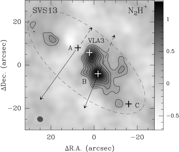
Figure 2: Image of the N₂H⁺(1–0) intensity integrated over the seven hyperfine line components for SVS 13. The unit of the scale is [Jy beam^-1 km s^-1]. Contours start at $\sim$ 3 $\sigma$ (see Table 1) with steps of $\sim$ 2 $\sigma$. Crosses represent the peaks of 3 mm dust continuum emission. Solid and dashed arrows show the direction of blue- and red-shifted outflows (see B98 and B2000). Dashed elliptical contour shows an approximate size of the large-scale common envelope. The synthesized PdBI beam is shown as grey oval.

Figure 2 shows the velocity-integrated N₂H⁺ intensity image of SVS 13, together with outflow information from B98 and B2000. The emission was integrated over all seven components of the N₂H⁺ line with frequency masks that completely cover velocity gradients within the object. A N₂H⁺ core, spatially associated with the mm continuum sources B and VLA 3, is found in the image. The core is elongated in the northeast-southwest direction and double-peaked: one peak is coinciding with source B and the other is located $\sim$ 2^′′ southwest to VLA 3. The FWHM radius of the whole core is measured to be $\sim$ 1520 AU. A jet-like extension is seen at the western edge of the core, which is $\sim$ 10^′′ in length and extending to northwest. Three smaller clumps (at $\sim$ 3–4 $\sigma$ level), one located close to source C and the other two located $\sim$ 10^′′ northeast of source A, are also seen in the image. We note that the small clumps towards northeast of source A are also seen in the BIMA + FCRAO N₂H⁺ image of NCG 1333 (see Walsh et al. 2007), and may be the remnant of a large-scale N₂H⁺ envelope (see $\S$ 4.4).

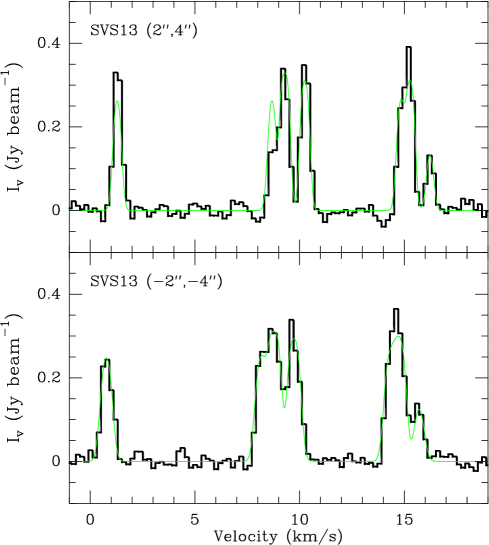
Figure 3: N₂H⁺ spectra at the two peak positions. Dotted curves show the results of hyperfine structure line fitting (see a color figure in the electronic version). Fit parameters are given in Table 3.

Figure 3 shows the N₂H⁺ (1–0) spectra at the two peak positions. All seven hyperfine lines of N₂H⁺ (1–0) have been detected. Using the hyperfine fitting program in CLASS, we derive LSR velocities ($V_{\rm LSR}$), intrinsic line widths ($\triangle$$v$; corrected for instrumental effects), total optical depth ($\tau_{\rm tot}$), and excitation temperatures ($T_{\rm ex}$) (see Table 3).

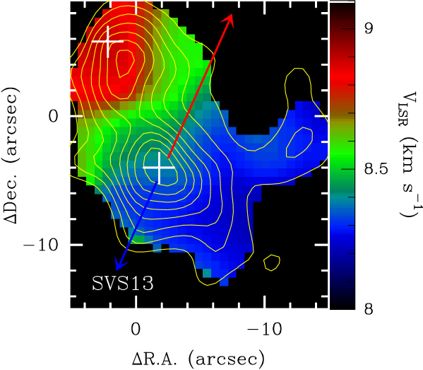
Figure 4: N₂H⁺ velocity field in SVS 13. Contours and crosses are the same as in Fig. 2. Red and blue arrows show the directions of red- and blue-shifted CO outflows.

By simultaneously fitting the seven hyperfine components with the routine described in Paper I, we derive the mean velocity field of SVS 13 (see Fig. 4). The outflow information (from B98) is also shown in the map. SVS 13 shows a well-ordered velocity field, with a smooth gradient from southwest to northeast. A least-squares fitting of the velocity gradient has been performed with the routine described in Goodman et al. (1993) and provides the following results: the mean core velocity is $\sim$ 8.6 km s^-1, the velocity gradient is 28.0 $\pm$ 0.1 km s^-1 pc^-1, and the position angle (P.A.) of the gradient is 51.3 $\pm$ 0.2 degree. The details of the velocity field are discussed in $\S$ 4.2.

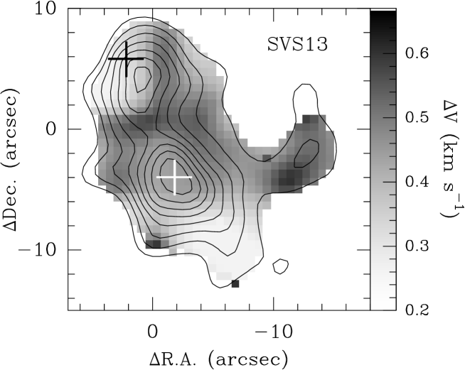
Figure 5: Spatial distribution of N₂H⁺ line widths in SVS 13, as derived from the HFS line fitting. Contours and crosses are the same as them in Fig. 2.

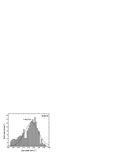
Figure 6: Distribution of N₂H⁺ line widths versus solid angle areas for SVS 13. Black solid curve and number show the results of Gaussian fitting to the distribution.

Figure 5 shows the spatial distribution of the N₂H⁺ line widths in the map. We find that the line widths are roughly constant within the core and large line widths are mainly seen in the gap between the two emission peaks and the jet-like extension at the core edge. The mean line width (0.48 $\pm$ 0.01 km s^-1) is derived from Gaussian fitting to the distribution of line widths versus solid angle area (see Fig. 6). The virial mass of the N₂H⁺ core is then estimated to be 0.7 $\pm$ 0.1 $M_{\odot}$, using the same method described in Paper II. The derived virial mass is slightly smaller than but still comparable to the total gas mass derived from the mm dust continuum images for source B.

3.2 Spitzer Results

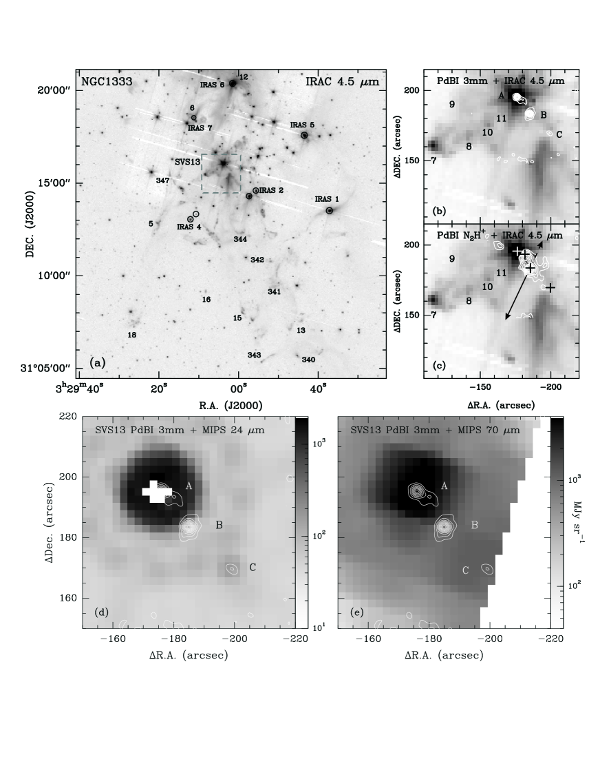
Figure 7: $Spitzer$ images of SVS 13. (a) $Spitzer$ IRAC band 2 (4.5 $\mu$m) image of SVS 13 (reference position at R.A.=03:29:17.49, DEC=31:12:48.54, J2000); (b) IRAC band 2 image overlaid with the PdBI 3 mm dust continuum contours; (c) Same as Fig. 7b, but overlaid with the PdBI N₂H⁺ intensity contours; (d) $Spitzer$ MIPS 1 (24 $\mu$m) image of SVS 13, overlaid with the PdBI 3 mm dust continuum contours; (e) Same as Fig. 7d, but for $Spitzer$ MIPS 2 (70 $\mu$m) image.

Figure 7 shows the $Spitzer$ images of SVS 13. In a wide-field IRAC 2 (4.5 $\mu$m) image shown in Fig. 7a, a number of HH objects are seen, implying active star formation in the NGC 1333 region. The HH objects that can be clearly distinguished are labeled by the same numbers as in Bally et al. (1996; for a comparison see optical image in their Figure 2). Figs. 7b and 7c show enlarged views of the 4.5 $\mu$m image, overlaid with the contours from the PdBI 3 mm dust continuum and N₂H⁺ images. In the IRAC maps, a strong infrared source is spatially coincident with the dust continuum source A. Located to the southeast of source A is the well-known HH chain 7$-$11 (see Fig. 7b), which is associated with a high-velocity blue-shifted CO outflow (B2000). Another collimated jet is found in the southern part of SVS 13 with the continuum source C being located at the apex (see Fig. 7b), but no near-infrared source is found at this position. Fig. 7c shows that the N₂H⁺ emission is not spatially associated with the infrared emission from source A, but extends roughly perpendicular to the directions of the jets/outflows.

In the MIPS 1 (24 $\mu$m) image, a strong infrared source (saturated in the image) is again found at the continuum source A, and another weak one is found at source C. In the MIPS 2 (70 $\mu$m) image, extended emission are seen at both sources A and C. It should be noted that no infrared emission is detected from source B in any IRAC or MIPS bands, suggesting that this source is a deeply embedded object. Flux densities of sources A and C are measured with aperture photometry in the IRAF APPHOT package, with the radii, background annuli, and aperture corrections recommended by the $Spitzer$ Science Center (see Table 4).

4 DISCUSSION

4.1 Spectral Energy Distributions and Evolutionary Stages

Figure 8 shows the spectral energy distributions (SEDs) of SVS 13 A, B, and C. IRAS far-infrared (only 100 $\mu$m data are used here) data are adopted from Jennings et al. (1987); SCUBA submm data from Chandler & Richer (2000); IRAM-30 m 1.3 mm data from Chini et al. (1997); BIMA 2.7 mm data from LMW2000; IRAM PdBI 3.1 mm data from this work and 3.5 mm data from B98. Since IRAS could not resolve SVS 13, the 100 $\mu$m flux ratio of A : B : C = 8:1:1 was inferred from the ratios at other wavelengths. For source B, the $Spitzer$ sensitivities at IRAC bands (also for source C) and MIPS bands are adopted.

In order to derive luminosities and temperatures, we first interpolated and then integrated the SEDs, always assuming spherical symmetry. Interpolation between the flux densities was done by a $\chi$² single-temperature grey-body fit to all points at $\lambda$ $\geq$ 100 $\mu$m, using the method described in Paper II. A simple logarithmic interpolation was performed between all points at $\lambda$ $\leq$ 100 $\mu$m. The fitting results are listed in Table 5.

The fitting results of sources B and C confirm the earlier suggestion (see e.g., Chandler & Richer 2000) that they are Class 0 protostars. For source A, the high bolometric temperature ($\sim$ 114 K) and low $L_{\rm submm}$/$L_{\rm bol}$ ratio ($\sim$ 0.8%) suggest it is a Class I young stellar object. Nevertheless, we want to note that source A resembles a Class 0 protostar in at least two aspects: (1) it is associated with a cm radio source (VLA 4; Rodríguez et al. 1999) and embedded in a large-scale dusty envelope, and (2) it is driving an extremely high velocity CO outflow (B2000), which is believed to be one of the characteristics of Class 0 protostars (see Bachiller 1996). We speculate that source A could be a Class 0/I transition object, which is visible at infrared wavelengths due to the high inclination angle (see B2000).

4.2 Gas Kinematics of the N₂H⁺ Core

4.2.1 Turbulence

Assuming that the kinetic gas temperature is equal to the dust temperature ($\sim$ 20 K; see Table 5), the thermal line widths of N₂H⁺ and an “average” particle of mass 2.33 m_H (assuming gas with 90% H₂ and 10% He) are $\sim$ 0.18 km s^-1 and $\sim$ 0.62 km s^-1, respectively. The latter line width represents the local sound speed. The non-thermal contribution to the N₂H⁺ line width ($\triangle v_{\rm NT}=\sqrt{\triangle v_{\rm mean}^{2}-\triangle v_{\rm th}^{2}}$) is then estimated to be $\sim$ 0.44 km s^-1, which is about two times larger than the thermal line width, but smaller than the local sound speed (i.e., subsonic).

It is widely accepted that turbulence is the main contribution to the non-thermal line width (Goodman et al. 1998), while infall, outflow, and rotation could also broaden the line width in protostellar cores. The spatial distribution of the line widths in SVS 13 (see Fig. 5) shows that large line widths ($\geq$ 0.45 km s^-1) only occur in the gap between sources B and VLA 3 and the jet-like extension at the edge of the core. At or around the two sources, line widths are relatively small (0.3 $-$ 0.4 km s^-1). Excluding the gap and extension, the re-estimated non-thermal line width would be $\sim$ 0.35 km s^-1. Although this is still larger than the thermal line width, it is fair to say that the turbulence in the SVS 13 core is at a low level.

4.2.2 Core Rotation

The velocity field map (Fig. 4) shows a clear velocity gradient across the core of $\sim$ 28 km s^-1 pc^-1 increasing from southwest to northeast, i.e., roughly along the connection line between sources B and VLA 3. As discussed in Paper I, systematic velocity gradients are usually dominated by either rotation or outflow. As seen in Fig. 4, the large angle ($>$ 70^∘) between the gradient and the outflow axis suggests that the observed velocity gradient in N₂H⁺ is due to core rotation rather than outflow.

The velocity gradient derived in SVS 13 is much larger than the results found in Papers I & II ($\sim$ 7 km s^-1 pc^-1) and other Class 0 objects, e.g., IRAM 04191 ($\sim$ 17 km s^-1 pc^-1; Belloche & André 2004), suggesting fast rotation of the N₂H⁺ core. With this gradient and the FWHM core size ($\sim$ 1520 AU), the specific angular momentum $J/M$ is calculated to be $\sim$ 0.47 $\times$ 10^-3 km s^-1 pc ($\sim$ 1.45 $\times$ 10¹⁶ m² s^-1), using the same method as described in Paper II. The ratio of the rotational energy to the gravitational potential energy is also calculated with the same method as described in Paper II, and the estimated $\beta_{\rm rot}$ value is $\sim$ 0.025 (uncorrected for inclination angle).

4.3 SVS 13 B and VLA 3: A Bound Protobinary System

Our observations show a weak 3 mm dust continuum source at the position of the radio source VLA 3 (see Fig. 1). This dust continuum source is embedded in the elongated N₂H⁺ core together with source B (see Fig. 2). The angular separation and flux ratio between sources B and VLA 3 are measured to be 10$\farcs$7 $\pm$ 0$\farcs$2 and $\sim$ 13 from the 3 mm dust continuum image, respectively.

The velocity field map shows a clear velocity gradient across the two sources, with sources VLA 3 and B being located in the red- and blue-shifted regions, respectively. As discussed above, we assume that this systematic velocity gradient is due to the core rotation. The two sources are thus probably forming a protobinary system that has originated from rotational fragmentation of the core that we now observe in the N₂H⁺ line.

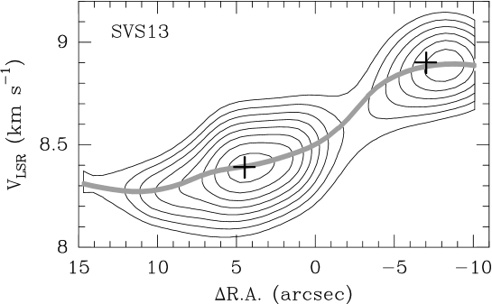
Figure 9: Position-velocity diagram of SVS 13 (along the connecting line between sources B and VLA 3). Crosses show the locations of sources B and VLA 3. The grey line marks the mean radial velocity.

Fig. 9 shows a position-velocity diagram, along the connecting-line between sources B and VLA 3. The radial velocity difference between the two sources is $\sim$ 0.5 km s^-1. Assuming that the two sources are in Keplerian rotation and that the orbit is circular and perpendicular to the plane to the sky, the velocity difference yields a combined binary mass of $\sim$ 1.1 $M_{\odot}$. Assuming a mass ratio of $\sim$ 13 ($M_{\rm B}$/$M_{\rm VLA3}$), the derived masses of sources B and VLA3 are 1.0 and 0.08 $M_{\odot}$, respectively. The estimated dynamical mass of source B is consistent with the total gas mass derived from the 1.4 mm dust continuum image (1.05 $M_{\odot}$). This in turn supports our assumption above that both sources B and VLA 3 are forming a bound binary system. Hereafter we refer to this binary protostar as the SVS 13 B/VLA 3 protobinary system. We also note that source A, which is much closer to VLA 3 in the 3 mm dust continuum image, is probably further away in foreground or background. This shows that 2-D images can be very misleading unless additional kinematic information like that derived from our N₂H⁺ observations is also considered.

4.4 Hierarchical Fragmentation in SVS 13:
Initial Fragmentation vs. Rotational Fragmentation

The 3 mm dust continuum image shows three distinct cores (A, B, and C) in SVS 13, which are roughly aligned along a line in the northeast-southwest direction (see Fig. 1). The morphology of the N₂H⁺ emission approximately follows this alignment. Nevertheless, there is an emission gap (hole) between the N₂H⁺ main core and the small clumps towards northeast of source A (see Fig. 2). This gap is possibly caused by an effect of the outflow, which releases great amounts of CO molecules and thus destroys N₂H⁺ around source A (see Aikawa et al. 2001 and also discussion in Paper II). The projected separations between sources A-B and B-C are $\sim$ 5000 AU and $\sim$ 7000 AU, respectively. Previous single-dish submm and mm maps show a large-scale common envelope with a radius of $\sim$ 20000 AU (0.1 pc), surrounding these three cores and elongated in the same direction (Chini et al. 1997; Chandler & Richer 2000). Based on these associated morphologies, we speculate that the three cores (A, B, and C) were formed by initial fragmentation of a large-scale filamentary prestellar core.

On the other hand, in the SVS 13 B sub-core, a binary protostar with a projected separation of 3800 AU is forming. The velocity field associated with this binary protostar is dominated by rotation and the ratio of rotational energy to gravitational energy is estimated to be $\beta_{\rm rot}$ $\sim$ 0.025. The $\beta_{\rm rot}$ value is believed to play an important role in the fragmentation process (see reviews by Bodenheimer et al. 2000 and Tohline 2002). Considering that magnetic fields support fragmentation, Boss (1999) has shown that rotating cloud cores fragment when $\beta_{\rm rot}$ $>$ 0.01 initially (but see also Machida et al. 2005). Based on this velocity structure, we suggest that the binary protostar in SVS 13 B is formed through rotational fragmentation of a single collapsing protostellar core.

Altogether we suggest a hierarchical fragmentation picture for SVS 13. (1) A large-scale filamentary prestellar core was initially fragmented into three sub-cores (sources A, B, and C) due to turbulence (see the review by Goodwin et al. 2007). (2) These sub-cores are continually contracting toward higher degrees of central condensation, and the rotation of the sub-cores is getting faster and dominates the gas motion instead of turbulence. (3) At a certain point, the condensations inside these sub-cores become gravitationally unstable and start to collapse separately to form either a binary protostar (e.g., SVS 13 A and B) if the rotational energy is larger than a certain level (e.g., $\beta_{\rm rot}$ $>$ 0.01) or a single protostar (e.g., SVS 13 C?) if the rotational energy is not high enough to trigger the fragmentation.

4.5 Accretion onto Protobinary: Simulations vs. Observations

Accretion onto a protobinary is one of the most important contributions to the final parameters of the system. Numerical simulations of accretion have found that the main dependencies are on the binary mass ratio and the relative specific angular momentum, $j_{\rm inf}$, of the infalling material (see Bate & Bonnell 1997 and Bate 2000). For unequal mass components, low $j_{\rm inf}$ material is accreted by the primary or its disk; for higher $j_{\rm inf}$, the infalling material can also be accreted by the secondary or its disk; when $j_{\rm inf}$ approaches the specific angular momentum of the binary system $j_{\rm B}$, circumbinary disk formation begins; when $j_{\rm inf}$ $\gg$ $j_{\rm B}$, the infalling material is accreted by neither component but only forms a circumbinary disk.

In our observations conducted at OVRO, ATCA and PdBI, we find in several protobinary systems that only one component is associated with a great amounts of circumstellar dust while the other is somewhat naked, e.g., SVS 13 B/VLA 3 (this work), CB 230 (Launhardt 2001; Launhardt et al. in prep.), and BHR 71 (Paper II). A similar situation was also found in the SVS 13 A protobinary system (Anglada et al. 2004). In fact, there is a trend derived from observations of only a very small number of sources (i.e., not a statistically significant sample) that unequal circumstellar masses (mass ratios below 0.5) protobinary systems are much more common than those equal masses systems (Launhardt 2004; Chen et al. in prep.). Since the detection bias goes towards equal-mass protobinary systems (e.g., sources VLA 1623, LMW2000 and L723 VLA2, Launhardt 2004), we consider this trend is not negligible. The large contrast between the two components implies that the accretion and hence development of a circumstellar disk occurs preferentially in only one component, with the disk absent or much less significant in the other one.

According to the definition in Bate & Bonnell (1997, hereafter BB97), we can calculate the specific orbital angular momenta of binary system as $j_{\rm B}$ = $\sqrt{GM_{\rm B}D}$ (where $G$, $M_{\rm B}$, and $D$ are the gravitational constant, total binary mass, and separation, respectively), and consider it as an unity. Taking SVS 13 B as an example, we assume $M_{\rm B}$ = 1.0 $M_{\odot}$ (see $\S$ 4.3) and $D$ = 3800 AU, and adopt the specifical angular momentum derived from the N₂H⁺ velocity field as $j_{\rm inf}$ ($\sim$ 1.5 $\times$ 10¹⁶ m² s^-1). We then derive $j_{\rm inf}$/$j_{\rm B}$ $\sim$ 0.1. This ratio is exactly corresponding to the simulated case that only circumprimary disk could be formed in an accreting protobinary system (see BB97). Therefore, the fact that only one component in a protobinary system is associated with a large amount of circumstellar material (or a circumstellar disk) could be explained by the relatively low specific angular momentum in the infalling envelope.

For a comparison, we list in Table 6 the corresponding parameters of L1551 IRS5, a well-studied protobinary system which we already knew the information of infalling gas and binary parameters (e.g., dynamical mass and separation). In contrast to SVS 13B, L1551 IRS5 apparently corresponds to a case of accretion of material with relatively higher angular momentum ($j_{\rm inf}$/$j_{\rm B}$ $\sim$ 1.0), and both components in the system are observed with a circumstellar disk (see Rodríguez et al. 1998), which is also consistent with the theoretical simulation in BB97. Nevertheless, so far the data which would reveal the link between specific angular momenta and formation of circumstellar disks are very rare, and no statistically significant correlations can be derived yet.

5 CONCLUSION

We present IRAM-PdBI observations in the N₂H⁺(1 $-$ 0) line and the 1.4 and 3 mm dust continuum toward the low-mass protostellar core SVS 13. Complementary infrared data from the Spitzer Space Telescope are also used in this work. The main results are summarized below:

(1) The 3 mm dust continuum image resolves four sources in SVS 13, named A, B, C, and VLA 3, respectively. Source C lies outside of the view at 1.4 mm, while source VLA 3 is not seen in the 1.4 mm continuum image. The separations between sources A-B and B-C are measured to be $\sim$ 5000 AU and $\sim$ 7000 AU, respectively. Assuming optically thin dust emission, we derive total gas masses of $\sim$ 0.2 $-$ 1.1 $M_{\odot}$ for the sources.

(2) N₂H⁺ (1–0) emission is detected in SVS 13. The emission is spatially associated with the dust continuum sources B and VLA 3. The excitation temperature of the N₂H⁺ line is $\sim$ 11 K. The FWHM radius of the N₂H⁺ core is $\sim$ 1520 AU. The line widths are roughly constant within the interiors of the core and large line widths only occur in the gap between the two dust continuum sources and a jet-like extension at the edge of the core. The observed mean line width is $\sim$ 0.48 km s^-1 and the derived virial mass of the N₂H⁺ core is $\sim$ 0.7 $M_{\odot}$.

(3) We derive the N₂H⁺ radial velocity field for SVS 13. The velocity field shows a systematic velocity gradient of $\sim$ 28 km s^-1 pc^-1 across the dust continuum sources B and VLA 3, which could be explained by rotation. We estimate the specific angular momentum of $\sim$ 0.47 $\times$ 10^-3 km s^-1 pc ($\sim$ 1.45 $\times$ 10¹⁶ m² s^-1) for this N₂H⁺ core. The ratio of rotational energy to gravitational energy is $\sim$ 0.025.

(4) Infrared emission from sources A and C is detected at $Spitzer$ IRAC bands and MIPS bands. Source A is driving a chain of HH objects, as seen in the IRAC 4.5 $\mu$m infrared image. No infrared emission is detected from source B in any $Spitzer$ bands, suggesting the source is deeply embedded.

(5) By fitting the spectral energy distributions, we derive the dust temperature, bolometric temperature, and bolometric luminosity for the sources A, B, and C. We find that sources B and C are Class 0 protostars, while source A could be a Class 0/I transition object.

(6) The velocity field associated with sources B and VLA 3 suggests that the two sources are forming a physically bound protobinary system embedded in a common N₂H⁺ core. The estimated dynamical mass of source B ($\sim$ 1.0 $M_{\odot}$) is consistent with its gas mass derived from the mm dust continuum images.

(7) Based on the morphologies and velocity structures, we suggest a hierarchical fragmentation picture for SVS 13: the three sources (A, B, and C) in SVS 13 were formed by initial fragmentation of a filamentary prestellar core, while the protobinary systems SVS 13 B/VLA 3 and SVS 13 A were formed by rotational fragmentation of the collapsing sub-cores.

(8) Our observations conducted at OVRO, ATCA, and PdBI find in several protobinary systems that only one component is associated with a large amount of circumstellar material while the other is somewhat naked, implying that the accretion and hence development of a circumstellar disk occurs preferentially in only one component, with the disk absent or much less significant in the other one. We find that this situation could be explained by the relatively low specific angular momentum in the infalling envelope, which is supported by both simulations and observations.

Table 1: IRAM-PdBI observation logs of SVS13.

Object	Other	R.A. & Dec. (J2000)a	Distance	Array	HPBWb	rmsc
Name	Name	[h : m : s, ${}^{\circ}:\,^{\prime}:\,^{\prime\prime}$]	[pc]	configuration	[arcsecs]	[mJy/beam]
SVS13	HH 7$-$11	03:29:03.20, 31:15:56.00	350	CD	2.8$\times$2.5, 1.2$\times$1.1	15.5, 0.62, 3.7

Table 2: PdBI mm dust continuum results for SVS 13.

Source	Positiona			$S_{\nu}$a,b [mJy]			FWHM sizes at 3 mma		$M_{\rm gas}$
	$\alpha$(J2000)	$\delta$(J2000)		$\lambda$3 mm	$\lambda$1.4 mm		maj.$\times$min.	P.A.	[$M_{\odot}$]
SVS 13 A	03:29:03.75	31:16:03.76		30.0$\pm$4.5	135$\pm$21		2$\farcs$4$\times$1$\farcs$4	–58$\pm$6°	0.75$\pm$0.12
B	03:29:03.07	31:15:52.02		42.4$\pm$6.4	193$\pm$30		2$\farcs$7$\times$1$\farcs$8	–46$\pm$5°	1.05$\pm$0.16
C	03:29:01.96	31:15:38.26		6.5$\pm$1.0	$--$		$\sim$ 0$\farcs$7	$--$	0.20$\pm$0.03

Table 3: Results of N₂H⁺ (1–0) spectra fitting^a

Peak [′′]	$V_{\rm LSR}$ [km s-1]	$\triangle$$v$ [km s-1]	$\tau_{\rm tot}$	$T_{\rm ex}$ [K]
(2, 4)	8.90$\pm$0.01	0.31$\pm$0.01	1.9$\pm$0.1	11.3$\pm$0.5
($-$2, $-$4)	8.39$\pm$0.01	0.46$\pm$0.02	2.2$\pm$0.1	10.1$\pm$0.5

Table 4: $Spitzer$ flux densities of SVS 13 A and SVS 13 C.

	R.A.a	Dec.a	$S(3.6\,\mu m)$	$S(4.5\,\mu m)$	$S(5.8\,\mu m)$	$S(8.0\,\mu m)$	$S(24\,\mu m)$	$S(70\,\mu m)$
Source	(J2000)	(J2000)	[mJy]	[mJy]	[mJy]	[mJy]	[Jy]	[Jy]
SVS 13 A	03:29:03.73	31:16:03.80	292$\pm$20	499$\pm$44	2470$\pm$140	2330$\pm$100	$>$ 21	112$\pm$3
C	03:29:01.98	31:15:38.17	$<$ 0.36b	$<$ 0.43b	$<$ 1.3b	$<$ 0.54b	0.22$\pm$0.01	$>$ 12

Table 5: Fitting results of the spectral energy distribution

Source	$T_{\rm dust}$	$T_{\rm bol}$	$L_{\rm bol}$	$L_{\rm submm}$	$L_{\rm submm}$/$L_{\rm bol}$	Class
	[K]	[K]	[$L_{\odot}$]	[$L_{\odot}$]	[%]
SVS 13 A	33	114	46.6	0.37	0.8	0/I(?)
B	22	28	5.6	0.28	5.0	0
C	20	36	4.9	0.13	2.7	0

Table 6: Specific angular momenta of envelopes and binaries

Source	Class	$j_{\rm inf}$a	Massb	Sepa.	$j_{\rm B}$	$j_{\rm inf}$/$j_{\rm B}$	Refs.c
		[m2 s-1]	[$M_{\odot}$]	[AU]	[m2 s-1]
L1551 IRS5	I	3.1$\times$$10^{16}$	1.2 (0.4)	40	3.0$\times$$10^{16}$	$\sim$1.0	1,2
SVS 13 B	0	1.5$\times$$10^{16}$	1.1 ($<$0.1)	3800	2.7$\times$$10^{17}$	$\sim$0.1	3

Figure 8: Spectral energy distributions of SVS 13 A (left), B (middle), and C (right). Error bars (1 $\sigma$) are indicated for all data points, but are mostly smaller than the symbol sizes. While most solid squares represent real observational data points, the 2.7$-$3.5 mm fluxes were measured from interferometric maps which resolved out the envelope and thus represent lower limits only. Open squares represent IRAS 100 $\mu$m data points, where flux densities are estimated for the three sources with ratios assumed in $\S$ 4.1. Open triangles represent the sensitivities of IRAC and MIPS. Solid lines show the best-fit for all points at $\lambda$ $\geq$ 100 $\mu$m using a grey-body model (see text). Dashed lines at $\lambda$ $\leq$ 100 $\mu$m show the simple logarithmic interpolation used to derive the luminosity. The fitting results are summarized in Table 5.

References

- Aikawa et al. (2001) Aikawa, Y., Ohashi, N., Inutsuka, S. I. et al. 2001, ApJ, 552, 639
- Anglada et al. (2004) Anglada, G. Rodríguez, L. F., & Osorio, M., et al. 2004, ApJ, 605, L137
- Anglada et al. (2000) Anglada, G. Rodríguez, L. F., & Torrelles, J. M. 2000, ApJ, 542, L123
- Bachiller (1996) Bachiller, R. 1996, ARA&A, 34, 111
- Bachiller et al. (2000) Bachiller, R., Gueth, F., Guilloteau, S., et al. 2000, A&A, 362, L33 (B2000)
- Bachiller et al. (1998) Bachiller, R., Guilloteau, S., Gueth, F., et al. 1998, A&A, 339, L49 (B98)
- Bally et al. (1996) Bally, J., Devine, D., & Reipurth, B. 1996, ApJ, 473, L49
- Bate (2000) Bate, M. R. 2000, MNRAS, 314, 33
- Bate & Bonnell (1997) Bate, M. R., & Bonnell, I. A. 1997, MNRAS, 285, 33
- Belloche & André (2004) Belloche, A., André, P. 2004, A&A, 419, L35
- Bodenheimer et al. (2000) Bodenheimer, P., Burkert, A., Klein, R. I., & Boss, A. P. 2000, in Protostars and Planets IV, ed. V. Mannings, A. P. Boss, & S. R. Russell (Tucson: Univ. Arizona Press), 675
- Boss (1999) Boss, A. P. 1999, ApJ, 520, 744
- (13) Chandler, C. J., & Richer, J. S. 2000, ApJ, 530, 851
- Chen et al. (2007) Chen, X. P., Launhardt, R., & Henning, Th. 2007, ApJ, 669, 1058 (Paper I)
- Chen et al. (2008) Chen, X. P., Launhardt, R., & Bourke, T., et al. 2008a, ApJ, 683, 862 (Paper II)
- Chen et al. (2008) Chen, X. P., Bourke, L. T., Launhardt, R., & Henning, Th., 2008b, ApJ, 686, L107
- Chini et al. (1997) Chini, R., Reipurth, B., & Sievers, A., et al. 1997, A&A, 325, 542
- Draine & Lee (1984) Draine, B. T., & Lee, H. M. 1984, ApJ, 285, 89
- Evans et al. (2003) Evans II, N. J., et al. 2003, PASP, 115, 965
- Goodman et al. (1998) Goodman, A. A., Barranco, J. A., Wilner, D. J., & Heyer, M. H. 1998, ApJ, 504, 223
- Goodman et al. (1993) Goodman, A. A., Benson, P. J., Fuller, G. A., & Myers, P. C. 1993, ApJ, 406, 528
- Goodwin et al. (2007) Goodwin, S., Kroupa, P., Goodman, A., & Burkert A. 2007, in Protostars and Planets V, ed. B. Reipurth, D. Jewitt, & K. Keil (Tucson: Univ. Arizona Press), 133
- Herbig (1974) Herbig, G. H. 1974, Lick Obs. Bull., 658
- Herbig & Jones (1983) Herbig, G. H. & Jones, B. F. 1983, AJ, 88, 1040
- Hirota et al. (2007) Hirota, T., Bushimata, T., & Choi, Y. K., et al. 2007, arXiv0709.1626
- Jennings et al. (1987) Jennings, R. E., Cameron, D. H. M., Cudlip, W., & Hirst, C. J. 1987, MNRAS, 226, 461
- Khanzadyan et al. (2003) Khanzadyan, T., Smith, M. D., Davis, C. J., et al., 2003, MNRAS, 338, 57
- Launhardt (2001) Launhardt R. 2001, in The Formation of Binary Stars, IAU Symp. 200, ed. H. Zinnecker, & R. D. Mathieu (San Francisco: ASP), 117
- Launhardt (2004) Launhardt, R. 2004, in IAU Symp. 221, Star Formation at High Angular Resolution, ed. M. G. Burton, R. Jayawardhana, & T. L. Bourke (San Francisco: ASP), 213
- Launhardt & Henning (1997) Launhardt, R., & Henning, Th. 1997, A&A, 326, 329
- Looney et al. (2000) Looney, L. W., Mundy, L. G., & Welch, W. J. 2000, ApJ, 529, 477 (LMW2000)
- Machida et al. (2005) Machida, M. N., Matsumoto, T., Hanawa, T., & Tomisaka, K. 2005, MNRAS, 362, 382
- Ossenkopf & Henning (1994) Ossenkopf, V., & Henning, Th. 1994, A&A, 291, 943
- Rodríguez (2004) Rodríguez, L. F. 2004, RevMexAA, 21, 93
- Rodríguez et al. (1997) Rodríguez, L. F., Anglada, G., & Curiel, S. 1997, ApJ, 480, L125
- Rodríguez et al. (1999) Rodríguez, L. F., Anglada, G., & Curiel, S. 1999, ApJS, 125, 427
- Rodríguez et al. (1998) Rodríguez, L. F. et al. 1998, Nature, 395, 355
- Saito et al. (1996) Saito, M., Kawabe, R., Kitamura, Y., & Sunada, K. 1996, ApJ, 473, 464
- Strom et al. (1974) Strom, S. E., Grasdalen, G. L., & Strom, K. M. 1974, ApJ, 191, 111
- Strom et al. (1976) Strom, S. E., Vrba, F. J., & Strom, K. M. 1976, AJ, 81, 314
- Tohline (2002) Tohline, J. E. 2002, ARA&A, 40, 349
- Walsh et al. (2007) Walsh, A. J., Myers, P., & Di Francesco, J. et al. 2007, ApJ, 655, 958