Pair vs many-body potentials: influence on elastic and plastic behavior in nanoindentation

Abstract

Molecular-dynamics simulation can give atomistic information on the processes occurring in nanoindentation experiments. In particular, the nucleation of dislocation loops, their growth, interaction and motion can be studied. We investigate how realistic the interatomic potentials underlying the simulations have to be in order to describe these complex processes. Specifically we investigate nanoindentation into a Cu single crystal. We compare simulations based on a realistic many-body interaction potential of the embedded-atom-method type with two simple pair potentials, a Lennard-Jones and a Morse potential. We find that qualitatively many aspects of nanoindentation are fairly well reproduced by the simple pair potentials: elastic regime, critical stress and indentation depth for yielding, dependence on the crystal orientation, and even the level of the hardness. The quantitative deficits of the pair potential predictions can be traced back (i) to the fact that the pair potentials are unable in principle to model the elastic anisotropy of cubic crystals; (ii) as the major drawback of pair potentials we identify the gross underestimation of the stable stacking fault energy. As a consequence these potentials predict the formation of too large dislocation loops, the too rapid expansion of partials, too little cross slip and in consequence a severe overestimation of work hardening.

I Introduction

Nanoindentation into crystalline materials is a complex process.Fischer-Cripps (2004); Gouldstone et al. (2007) When the indenter is moved into the surface, it deforms the substrate first elastically, until a sufficiently high pressure has been established and plasticity sets in. This so-called ‘critical indentation depth’ is characterized by the critical stress necessary for the nucleation of dislocations. Upon further indentation, the emerging plasticity will initially lead to a drop in the contact pressure felt by the indenter – the ‘load drop’ – but then the contact pressure will saturate; its value is then called the hardness of the material. As soon as dislocations have been generated, they will propagate, multiply, cross-slip, interact with each other, etc. The multitude of the processes which these dislocations undergo will eventually have a back reaction on the proceeding indenter: the indenter will not penetrate into virgin material but into work hardened material.

Molecular-dynamics simulation has been employed to obtain a detailed in-depth understanding of the processes occurring during nanoindentation, and in particular in the plastic regime.Landman et al. (1990); Kelchner et al. (1998); Smith et al. (2003); Van Vliet et al. (2003); Li (2007); Szlufarska (2006); Gouldstone et al. (2007) The advantage of this method is the detailed atomistic information it can provide on virtually all the processes occurring in the material, and in fact, since the 1990s, an increasing number of simulations have been performed and contributed to our understanding of nanoindentation and plasticity in general. The use of these simulations is impeded by the large simulation volumes which are necessary to host the defects formed, and the long time scales over which simulations need to be followed. Besides these problems, in principle, molecular-dynamics simulation allow a realistic simulation of the events as long as the interatomic interaction potential has been realistically chosen.

One of the objectives of understanding the physics of nanoindentation is to trace back the origin of the physical phenomena observed to the peculiarities of the interatomic interaction for the specific material under investigation. The question then rises which feature of the interatomic interaction potential is responsible for which phenomenon observed in the simulation. Such questions can usually be answered with the help of sensitivity studies, in which one or several features of the interatomic potential are systematically varied and their effect on the simulation results is studied. Unfortunately, realistic interaction potentials, such as they are used nowadays, do not allow for such systematic changes, since they are available either in the form of parameterized analytical formulae, in which the change of one parameter affects several physical material properties simultaneously, or even only in the form of numerical tables. Therefore, simpler generic potentials may be employed which allow the typical behavior of solids to be studied without reproducing too well the specific properties of one particular material.

In particular, pair potentials have been used to model nanoindentation of materials or the related phenomena of plasticity, work hardening and material failure.Hoover et al. (1990); Holian et al. (1991); Kallman et al. (1993); Abraham et al. (2002a, b); Ma and Yang (2003); Buehler et al. (2004, 2005); Shi and Falk (2005) It has been known for long that pair potentials are capable to model rare gas solids, but they have several deficits in modelling metallic materials. Thus they allow to prescribe only two – rather than three – elastic constants for solids, they model an outwards – rather than an inwards – surface relaxation, etc.Carlsson (1990); Daw et al. (1993) However, how well are these pair potentials able to model nanoindentation? In other words, which aspects in the elastic and plastic deformation of the material, in the nucleation and glide of dislocations are described qualitatively correctly, and which are not? How large will quantitative deviations between the predictions of a pair potential and that of realistic potentials be?

In the present paper, we wish to answer these questions for the specific case of nanoindentation into a Cu single crystal. For this material, a many-body potential is available, which is well characterized also with respect to the prediction of the mechanical properties, enjoys a rather wide acceptance in the community, and which has been repeatedly used for nanoindentation and plasticity simulations in the past. We shall use simulations with this potential as a reference case and contrast the results obtained with those predicted by using two simple pair potentials.

II Method

II.1 Potentials

We chose the potential developed by Mishin et al.Mishin et al. (2001) as the state-of-the-art reference potential for Cu; this potential has been often employed for molecular-dynamics simulations and has been well characterized.Zhu et al. (2004); Tschopp et al. (2007); Tschopp and McDowell (2008); Liu et al. (2008) This potential belongs to the class of embedded-atom-method (EAM) potentials,Daw and Baskes (1984); Daw et al. (1993) which incorporate many-body bonding effects in an appropriate form to describe metallic bonding. In the embedded-atom method, the total energy of a system is represented as

$$E_{\rm tot}=\sum_{\begin{subarray}{c}i,j\\ i\neq j\end{subarray}}V_{\rm EAM}(r_{ij})+\sum_{i}F(\rho_{i}),$$ (1)

where $V_{\rm EAM}(r_{ij})$ is a pair potential evaluated as a function of the distance $r_{ij}$ between atoms $i$ and $j$, and $F$ is the embedding energy, which depends on the so-called ’electron density’ $\rho_{i}$. The latter is given by

$$\rho_{i}=\sum_{j\neq i}g(r_{ij}),$$ (2)

where $g(r_{ij})$ is the contribution of atom $j$ to the total electron density at the site of atom $i$. The detailed form of the functions $V_{\rm EAM}$, $F$, and $g$ is presented in Ref. Mishin et al., 2001. We collect in Table I a number of basic characteristics of crystalline Cu: the cohesive energy $E_{\rm coh}$, the lattice constant $a$, the bulk modulus $B$, and the three elastic moduli $c_{11}$, $c_{12}$ and $c_{44}$. These properties are well reproduced by the Mishin potential.

We employ two well known pair potentials, the Morse and the Lennard-Jones (LJ) potential. The Morse potential

$$V_{\rm Morse}(r)=D\left[e^{-2\alpha(r-r_{0})}-2e^{-\alpha(r-r_{0})}\right]$$ (3)

is characterized by three parameters: the bond strength $D$, the equilibrium bond distance $r_{0}$, and the potential fall-off $\alpha$. We fit these parameters to three materials properties; these are traditionally chosen as the lattice constant $a$, the cohesive energy $E_{\rm coh}$, and the bulk modulus $B$. The latter is given in terms of the elastic moduli by

$$B=\frac{c_{11}+2c_{12}}{3}.$$ (4)

For Cu, the parameters read $D=0.3282$ eV, $r_{0}=2.8985$ Å, and $\alpha=1.3123$ Å^-1. As Table I, demonstrates, the two elastic constants $c_{11}$ and $c_{12}$ are reproduced rather well, within a 2 % error margin. Of course, since pair potentials obey the Cauchy relationship,Carlsson (1990) $c_{44}=c_{12}$, it is not possible to fit $c_{44}$ separately, and indeed the shear modulus is misrepresented by almost 60 %.

For the LJ potential,

$$V_{\rm LJ}(r)=4\epsilon\left[\left(\frac{\sigma}{r}\right)^{12}-\left(\frac{\sigma}{r}\right)^{6}\right],$$ (5)

only two material parameters can be fitted. As the length parameter $\sigma$ only sets the length scale, it is used to fit the lattice constant $a$. Conventionally, the energy parameter $\epsilon$ is fitted to the cohesive energy $E_{\rm coh}$;Brüesch (1982) for the present work, however, the elastic properties are more important, and we hence fit $\epsilon$ to the bulk modulus $B$. Our fit parameters thus read: $\epsilon=0.1515$ eV and $\sigma=2.338$ Å. Table I proves that the cohesive energy is severely underestimated in this potential, while the two elastic moduli $c_{11}$ and $c_{12}$ are reproduced fairly well, within 12 %. In the conventional fitting scheme, which reproduces $E_{\rm coh}$ by setting $\epsilon=0.45$ eV, the bulk modulus – and hence the elastic moduli in general – are overestimated by a factor of 3.

We note that the LJ potential obeys a simple scaling property, which allows us to extend the results obtained in the present study to other systems by scaling lengths to $\sigma$ and energies to $\epsilon$. In this sense the results obtained for the LJ potential are ‘universal’.

Both pair potentials are smoothly cut off at $r_{\rm cut}=6.4$ Å, i.e., after the 6th neighbour shell. We chose the following procedureVoter (1993) – here described for the LJ potential –

$$V(r)=V_{\rm LJ}(r)-V_{\rm LJ}(r_{\rm cut})+{V_{\rm LJ}}^{\prime}(r_{\rm cut})\frac{r_{\rm cut}}{m}\left[1-\left(\frac{r}{r_{\rm cut}}\right)^{m}\right],$$ (6)

where the prime $V_{\rm LJ}^{\prime}$ denotes differentiation with respect to $r$, and a value of $m=20$ has been adopted. For the Morse potential, we proceed analogously.

II.2 Generalized stacking fault energy

Dislocations in fcc metals consist of two partial dislocations between which a stacking fault extends. The ability of potentials to describe the formation and the energetics of a stacking fault is therefore crucial when modelling plasticity. These features are conventionally described with the help of the so-called ‘generalized stacking fault energy’ of the crystallographic (111) plane. It is defined as follows.Vitek (1968) Consider an ideal lattice with total energy $E_{0}$. We cut it along a (111) plane into two halves. The upper half is shifted parallel to the bounding (111) plane with respect to the lower half by a vector

$$\vec{f}=\alpha\vec{a}+\beta\vec{b}\qquad 0\leq\alpha,\beta<1.$$ (7)

Here the vectors $\vec{a}$ and $\vec{b}$ span the (111) surface: $\vec{a}=\frac{1}{2}[11\bar{2}]$, $\vec{b}=\frac{1}{2}[1\bar{1}0]$.

The generalized stacking fault energy is then defined in terms of the energy $E(\alpha,\beta)$ of the distorted crystal as

$$\gamma(\alpha,\beta)=E(\alpha,\beta)-E_{0}.$$ (8)

For calculating the energy of the distorted crystal, a conjugate-gradient method is used; quenching will lead to the same numerical results. All particles are constrained to move only in the normal direction. It is crucial to choose the crystal sufficiently large in the direction normal to the stacking-fault plane in order to obtain stable solutions; unstable solutions lead to a discontinuous energy surface. We chose a size of 10 unit cells in the lateral directions, and 25 unit cells for each half-crystal in normal direction.

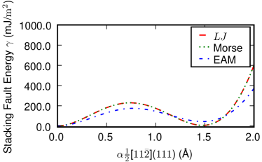
Figure 1: Generalized stacking fault energy $\gamma$ along the $\langle 11\bar{2}\rangle$ {111} direction.

In Fig. 1 we display the generalized stacking fault energy in $\langle 11\bar{2}\rangle$ {111} direction. The values of the stable stacking fault energy $\gamma_{s}$ and of the unstable stacking fault energy $\gamma_{u}$ – that is the energy barrier between the undistorted lattice position and the stacking fault position – are also assembled in table II. We note that the values for $\gamma_{u}$ predicted by the three potentials are not too far from each other; this demonstrates that the value of the bulk modulus – which has been chosen identical in the three potentials – has a major influence on the value of $\gamma_{u}$. Quantitatively, the Morse (LJ) potential predicts a value of $\gamma_{u}$ which is by 17 % (31 %) too high in comparison with the prediction of the EAM potential; we note that no experimental value for this quantity is available. The values of the stable stacking fault energy $\gamma_{s}$ vary quite dramatically from each other. We note that the EAM potential predicts a value which is quite close to the experimental valueCarter and Ray (1977) of 45 mJ/m². The values of $\gamma_{u}=5.9$ mJ/m² for the Morse potential and of 10.8 mJ/m² for the LJ potential are considerably too small. The fact that the stable stacking fault energy is so small is not untypical of pair potentials. For the LJ potential, for instance, it is well known that for infinite cutoff radius, $r_{\rm cut}=\infty$, the hcp phase has almost identical (in fact, even smaller) energy as the fcc phase;Barron and Domb (1955); Wallace and Patrick (1965) even though differences between the two phases become larger for finite cutoff radius,Jackson et al. (2002) this fact makes a small value of $\gamma_{s}$ plausible.

II.3 Simulation

We employ the method of classical molecular-dynamics to model the indentation process. Our substrate consists of an fcc crystal. In the case of a (100) surface, it has a side length of 70 lattice constants in all directions and contains 1,372,000 atoms. In the case of the (111) surface, similar crystal dimensions have been chosen, and the crystal contains 1,381,800 atoms. We checked in a series of simulations that our crystallite size is large enough to obtain reliable results for the indentation process by investigating the force and pressure depth curves, atomistic snapshots and the defect dynamics.

Lateral periodic boundary conditions have been applied. At the bottom, atoms in a layer of the width $r_{\rm cut}$ have been constrained to $F_{\rm normal}=0$; we checked that increasing the width of this layer to $(2\dots 3)r_{\rm cut}$ – as it is appropriate for the EAM potential – has no influence on the results of our indentation simulations. The simulations have been done in the microcanonical ensemble at $T=0$ K using a modified version of the LAMMPS code.LAM

We found that a careful relaxation of the crystal before starting the indentation process is crucial in order to obtain reliable and reproducible results. The substrate has been relaxed to $p_{ij}<10^{-5}$ GPa and temperatures $\ll 1$ K using a very low frictional force and pressure relaxation in a Nose-Hoover algorithm. Upon incomplete relaxation, we encountered artefacts like oscillations in the response functions during the indentation process and an overestimation of the material strength; these features are caused by the remaining internal stress fields in the crystal.

The indenter is modelled as a repulsive soft sphere. We chose a non-atomistic representation of the indenter, since we are not interested in the present study in any atomistic displacement processes occurring in the indenter, but only in the substrate. The interaction potential between the indenter and the substrate atoms is limited to distances $r<R$, where $R$ is the ‘indenter radius’. At $r<R$, the potential smoothly increases likeKelchner et al. (1998)

$$V(r)=\left\{\begin{array}[]{ll}k(R-r)^{3},&r<R,\\ 0,&r\geq R.\end{array}\right.$$ (9)

We call $k$ the indenter stiffness. For the results presented here, it has been set to $k=3$ eV/ų. We checked that our results are only weakly influenced by the exact value of the contact stiffness, as long as it is in the range of $1-10$ eV/ų. Only when decreasing $k$ to below 0.1 eV/ų, the results change sensitively; this can be understood since the decreased indenter stiffness translates into a smaller indenter ‘elastic modulus’.

Our indenter has a radius of $R=8$ nm. This value was chosen as a compromise; for larger indentation radii, the influence of the finite size of the simulation volume shows up, while with decreasing $R$, the atomistic nature of the indentation process leads to increased fluctuations, in particular in the contact area. We made sure in a series of simulations, that in the range of $R=3-15$ nm in the elastic regime, no systematic deviations from the Hertzian theory appear.

We tested two methods of indentation, a displacement-controlled and a velocity-controlled approach. When controlling the displacement, we advance the indenter every $\Delta t=2$ ps by a fixed amount of $\delta=0.256$ Å ($\ll$ lattice constant) instantaneously, corresponding to an average indentation speed of $v=12.8$ m/s. The substrate then relaxes for the ensuing time of $\Delta t$ to the new indenter position. In the velocity-controlled method, a fixed indentation speed of $v=12.8$ m/s is imposed on the indenter. We found no systematic differences in the material response nor in the induced plasticity between the simulation results obtained by the two methods. We prefer to use the former method. We note that in experiment, either displacement or force can be controlled.Fischer-Cripps (2004) In the following all ensemble properties are obtained by averaging over the $2$ ps relaxation cycle. All our simulations were performed without damping; the resulting energy input into the crystal amounted to less than 6 meV/atom.

III Results

III.1 Elastic regime: load-displacement curves

In Fig. 2 we display the basic information obtained from nanoindentation simulation, the force-displacement curves. For the two crystal surfaces studied, the (100) and the (111) surface, the three potentials give results which are qualitatively in agreement with each other. However, in detail deviations are visible which will be discussed in the following.

Let us first look at the elastic regime which is well described by the Hertzian law,Hertz (1882); Fischer-Cripps (2004)

$$F=\frac{4}{3}E_{r}d^{3/2}\sqrt{R}.$$ (10)

Here, $E_{r}$ is the so-called indentation modulus, which for an isotropic solid can be expressed as

$$E_{r}=\frac{E}{1-\nu^{2}}$$ (11)

in terms of the Young modulus $E$ and the Poisson ratio $\nu$ of the material. However, the material discussed here is strongly anisotropic. The anisotropy of cubic materials can be expressed in terms of the elastic moduli via

$$A=\frac{2c_{44}}{c_{11}-c_{12}},$$ (12)

Its value is presented in Table III. Due to the fact that the pair potentials do not model all three elastic constants, they predict wrong values for the anisotropy; however, in all potential models discussed here, Cu is strongly anisotropic.

Vlassak and NixVlassak and Nix (1993, 1994) have shown that in an anisotropic solid, the Hertzian force-displacement law (10) remains valid if an orientation-dependent indentation modulus $E_{r}(\mathbf{\Omega})$ is appropriately chosen; they give numerical tables to evaluate $E_{r}(\mathbf{\Omega})$ as a function of the elastic constants. We collect the results evaluated for our potentials in Table III. It is seen that the (111) surface is stiffer than the (100) surface. As expected, the EAM results are in close agreement with the moduli calculated using the experimental data. For the (100) direction, the Morse potential yields indentation moduli which fairly well reproduce those of the EAM potential, while the LJ potential is considerably – by 41% – too stiff. For the (111) surface also the Morse prediction overestimates (by 40 %) the indentation modulus; this is due to the fact that the anisotropy $A$, which is only poorly represented by the pair potentials, sensitively enters the modulus in this direction.

In table III, we also display fit values $E_{r}^{\rm fit}$ for the indentation moduli, which have been obtained by fitting Fig. 2 to the Hertzian law, Eq. (10). We perform this fit only for the initial part of the indentation curve ($d<2$ Å) in order to stay in the regime of linear elasticity. When we compare with the indentation moduli, we see an overall fair agreement with at most 12 % deviation. We attribute these minor deviations to (i) the atomistic nature of the indentation process, which for the indenter radius of 8 nm is not fully captured by continuum elasticity; (ii) the possible onset of nonlinear elastic processes – as these tend to make the material respond more stiffly to the applied force,Zhu et al. (2004) this would agree with our finding that most fitted moduli are larger than the theoretical prediction; (iii) the numerical problem of fitting the molecular-dynamics data to the Hertzian law – note that besides the elastic deformation also a finite offset in the displacement has to be fitted. We conclude that the Vlassak-Nix indentation moduli give an at least semi-quantitatively correct representation of the elastic behavior of the three potentials, and allows us to understand the trends in the elastic part of the force-displacement curves in Fig. 2.

III.2 Onset of plasticity

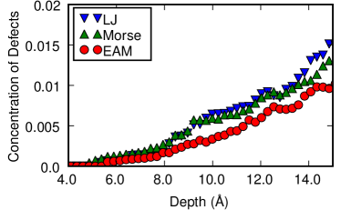
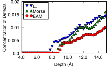
Figure 10: Concentration of Stacking Faults, i.e., fraction of atoms occupying stacking-fault sites. Crystal orientation: a) (100) b) (111).

In order to discuss the onset of plasticity and hardness, the evolution of the contact pressure is displayed in Fig. 3. These data are obtained from the forces $F$ of Fig. 2 by dividing through the pertinent projected contact areas. For the (111) surface, the critical indentation depth $d_{\rm yield}$ can be quite clearly identified at around $8-10$ Å; after this indentation, plasticity sets in (see also Fig. 10 below). The contact pressure at $d_{\rm yield}$ is called the critical stress $\sigma_{\rm cr}$. When $d_{\rm yield}$ is exceeded, a quite considerable load drop is experienced for the (111) surface, which corresponds to a softening of the material due to the production of mobile defects. For the (100) surface, the onset of plasticity is not as sharp and already starts at around 5 Å, cf. also Fig. 10 discussed below.

These principal features of the two surfaces are qualitatively well reproduced by all three potentials. The origin of the abrupt onset of plasticity for the (111) surface is twofold: (i) the primary glide systems $\langle 1\bar{1}0\rangle$ {111} are located at quite oblique angles to the direction of the indentation force acting normally to the surface; the corresponding Schmid factor is only $s_{111}=\sqrt{2/27}=0.27$. For the (100) surface these glide systems are more easily activated, since $s_{100}=1.5s_{111}=1/\sqrt{6}=0.41$. (ii) When finally the critical indentation depth has been reached, a considerable elastic energy has built up due to the high stiffness of this surface. Then, upon dislocation nucleation, a stronger dislocation avalanche and consequently a larger plastic displacement jump are achieved.

The values of the critical stresses obtained in the simulation are assembled in table IV. At these stresses, the resolved shear stress on the slip plane exceeds the theoretical shear strength – that is the maximum shear stress that a defect-free solid can sustain without yielding – of the crystal. The theoretical strength $\tau_{\rm th}$ of an fcc single crystal has been calculated by FrenkelFrenkel (1926); Kelly and Macmillan (1986) as

$$\tau_{\rm th}=\frac{1}{\sqrt{2}}\frac{1}{2\pi}{G_{r}}^{\prime},$$ (13)

where ${G_{r}}^{\prime}$ is the (so-called ‘relaxed’)Kelly and Macmillan (1986); Roundy et al. (1999) shear modulus for the preferred glide system $\langle 1\bar{1}0\rangle$ {111} that is calculated from the elastic constants asFrenkel (1926); Kelly and Macmillan (1986)

$${G_{r}}^{\prime}=\frac{3c_{44}(c_{11}-c_{12})}{4c_{44}+c_{11}-c_{12}}.$$ (14)

In Eq. (13) we also take the fact into account that the interplanar distance of the glide planes is larger than the partial Burgers vector by a factor of $1/\sqrt{2}$.Kelly and Macmillan (1986)

Recent ab initio calculations of the theoretical strength of Cu (and other fcc metals) indicate that Frenkel’s estimate (13) is quite accurate; they only substitute the prefactor $1/\sqrt{2}2\pi=0.11$ by 0.085;Roundy et al. (1999); Ogata et al. (2002, 2004) for the present purposes it will be sufficient to stay with Frenkel’s original estimate (13). The values of ${G_{r}}^{\prime}$ and $\tau_{\rm th}$ predicted by the potentials are included in table IV.

For an anisotropic crystal, it is a nontrivial task to establish a quantitative relationship between the theoretical strength $\tau_{\rm th}$ of the solid – that is the maximum shear stress that a defect-free solid can sustain without yielding – and the critical stress $\sigma_{\rm cr}$, as it is applied in a nanoindentation experiment on the surface of the crystal. For isotropic solids, this relationship has been analyzed and it has been found that for a material with a Poisson ratio of 0.3, the maximum shear stress occurs along the axis of symmetry at a depth of approximately $a/2$, where $a$ is the radius of the contact area.Tabor (1951); Johnson (1985); Fischer-Cripps (2007) At this point, the shear stress is given by

$$\tau=0.47\sigma,$$ (15)

where $\sigma$ is the contact pressure, i.e., the mean stress on the surface. This maximum shear acts on planes inclined to the surface at $45^{\circ}$. Since this resembles the situation of a solid under uniaxial stress, the Schmid factor might be expected to provide a valid though rough estimate of the maximum resolved shear stress on the slip planes underneath the indenter. This reasoning would lead to the prediction that the critical stresses should behave in inverse proportion to the relevant Schmid factors

$$\frac{\sigma_{\rm cr}(111)}{\sigma_{\rm cr}(100)}=\frac{s_{100}}{s_{111}}=1.5.$$ (16)

As Table IV shows, indeed $\sigma_{\rm cr}(111)>\sigma_{\rm cr}(100)$, but the ratio is only around $1.2-1.3$, rather than 1.5. Since the Schmid factors simply express the geometric orientation of the slip systems with respect to the surface plane, the disagreement of the molecular-dynamics results with the prediction (16) indicates that the stress state inside an anisotropic material looks rather different from the above simple reasoning. If we nevertheless attempt to use the isotropic result (15) to connect the external average stress on the surface to the internally active shear stress, and naively include the Schmid factor to take the surface orientation into account, we arrive at

$$\sigma_{\rm cr}=\frac{1}{0.47s}\tau_{\rm th}=\left\{\begin{array}[]{ll}5.2\tau_{\rm th},&(100),\\ 7.9\tau_{\rm th},&(111).\end{array}\right.$$ (17)

A comparison with table IV shows that this result allows to explain satisfactorily the order of magnitude of the critical stresses observed. When we consider furthermore the value of the critical stresses for the different potentials, we see that the critical stress of the LJ potential is highest (this fact agrees with the overestimation of the elastic properties), while those of the Morse and the EAM potentials are quite similar, despite the difference in the unstable stacking fault energies in these potentials.

The critical indentation depths for the different potentials show the inverse behavior. Since the contact pressure rises strongest for the LJ potentials the critical indentation depth is the smallest, while for Morse and EAM potential it has almost the same value. Overall, the differences in the critical indentation depths are not as pronounced as those for the critical stresses.

For the (100) surface, the discussion of the critical indentation depth is not useful due to the very smooth onset of dislocation nucleation. We note, however, that at a depth of around $8-10$ Å, also for this surface the maximum stress is observed for the EAM and LJ potentials, which is of similar size as the critical stress in the (111) surface. Upon further indentation, however, no load drop is experienced, but only a drop in contact pressure. This feature is due to the considerable increase in dislocations observed at this point, see also Fig. 10 below.

III.3 Hardness

The contact pressure which has been established after the critical indentation depth has been exceeded and a possible load drop has occurred, stays rather constant with increasing indentation; this defines the hardness of the material. Fluctuations in this regime are due to the atomistic resolution of the processes and immediately reflect the generation and interaction of dislocations with each other. Note that the hardness for the EAM potential remains rather constant, while that of the pair potentials tends to increase somewhat with increasing indentation depth. This feature is particularly pronounced for the LJ potential and reflects the work hardening of the material due to the high density of partial dislocations with extended stacking faults, cf. Sect. III.4 below.

III.4 Atomistic Snapshots

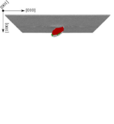
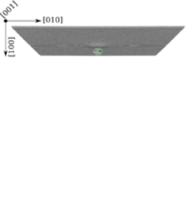
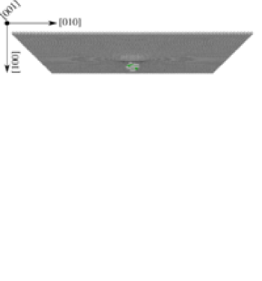
Figure 4: Snapshots of embryonic plasticity ($d=5.6$ Å) for (100) Cu. a) LJ b) Morse c) EAM potential.

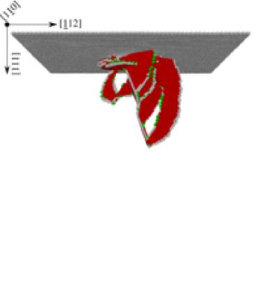
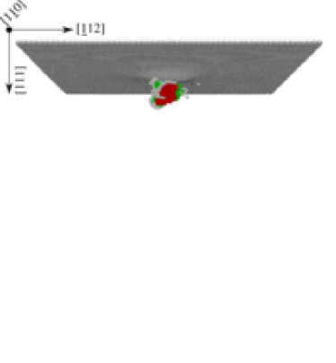
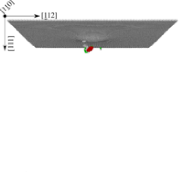
Figure 5: Snapshots of embryonic plasticity ($d=8.7$ Å) for (111) Cu. a) LJ b) Morse c) EAM potential.

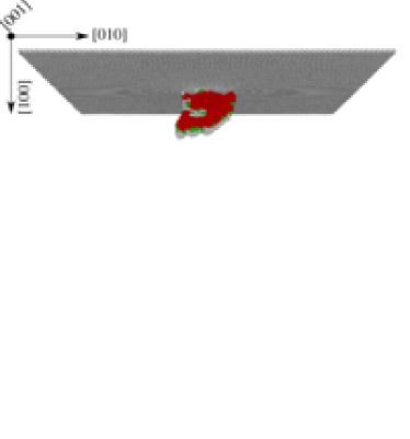
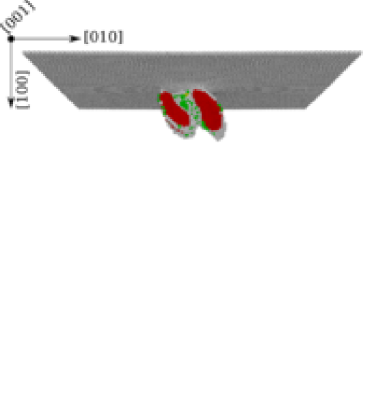
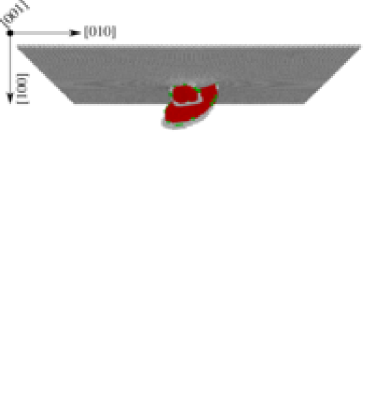
Figure 6: Snapshots of emerging plasticity ($d=8.2$ Å) for (100) Cu. a) LJ b) Morse c) EAM potential.

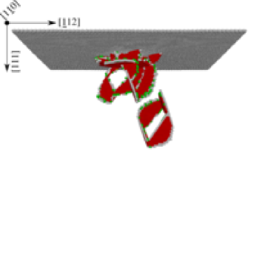
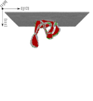
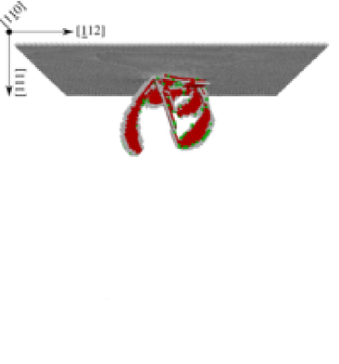
Figure 7: Snapshots of emerging plasticity ($d=9$ Å) for (111) Cu. a) LJ b) Morse c) EAM potential.

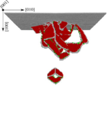
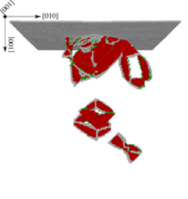
Figure 8: Snapshots of fully developed plasticity ($d=14.1$ Å) for (100) Cu. a) LJ b) Morse c) EAM potential.

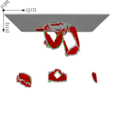
Figure 9: Snapshots of fully developed plasticity ($d=14.1$ Å) for (111) Cu. a) LJ b) Morse c) EAM potential.

We present in Figs. 4 – 9 atomistic views of the defects created in the material during the indentation process. These views have been obtained at different penetration depths: (i) ’Embryonic plasticity’, obtained immediately at the critical indentation depth, Figs. 4 and 6; (ii) ‘emerging plasticity’, where the dislocations formed are clearly discernible, but are still, more or less, localized under the indenter; and (iii) ’fully-developed plasticity’, where the dislocations have started to glide away from their point of production and fill the simulation volume. The plots have been generated using the recently developed algorithm by Ackland and Jones.Ackland and Jones (2006) This algorithm classifies all atoms according to their atomic neighborhood. In our case, we have fcc atoms (these constitute the vast majority of atoms and are not displayed for clarity), surface atoms (grey), and stacking fault atoms with a local hcp structure (red). All other atoms are categorized as atoms of lower symmetry and plotted in green. The boundaries of dislocations, positions where dislocations interact, and also embryonic defects are shown in this color.

Fig. 4 captures embryonic plasticity for the (100) surface just at the stage of homogeneous dislocation nucleation. For the Morse and EAM potential, the nucleating defect structures have not even formed stacking faults that could have been recognized by the detection algorithm. In the LJ potential, nucleation occurred somewhat earlier but at higher stresses than in the EAM case, cf. Fig. 10 discussed below. In all cases the nucleation process is seen to start homogeneously under the indenter, viz. in the region of highest shear stress on the (111) slip planes with highest resolved shear stress. For the (111) surface, Fig. 5, an instance of time has been selected where the nucleated dislocations are clearly discernible by their stacking fault planes. A comparison of Fig. 4 and 5 demonstrates that indeed the LJ system develops the largest stacking fault planes. This is connected to the extremely low stable stacking fault energy $\gamma_{s}$ of the LJ potential, which allows partial dislocations to propagate more easily.

The indentation depths of Figs. 6 and 7 have been chosen such that the dislocations are still localized in the region of highest shear stress under the indenter. Here, again the unrealistically large stacking fault planes obtained for the LJ potential (Fig. 6a) are seen; in Fig. 7b also the Morse potential has formed large stacking faults. Note, however, that for the (111) surface the defect structures for the three potentials look more similar to each other. Characteristically, for the realistic EAM potential, the emission of a prismatic loop is already seen at this stage, Fig. 6c. This already points at an easier possibility for cross slip occurring under this potential and is connected to the fact that work hardening occurs in the defective region. This feature will show up again in the case of fully developed plasticity.

For fully developed plasticity, Figs. 8 and 9, the emission of prismatic loops is observed for all potentials. For the LJ potential depicted in Fig. 9a a strikingly large number of prismatic loops is emitted. Again, dislocations in the LJ system are characterized by huge stacking faults. In the case of the pair potentials, in addition an exceptionally high number of V-shaped dislocations at the surface an be seen: a small one in Fig. 8a, and huge ones in Fig. 9b. These dislocations are prismatic loops moving parallel to the surface, and contain a higher core energy density than those in bulk material.

In summary, we can rationalize our atomistic results on the development of plasticity for the potentials investigated here using two concepts: (i) The extremely low stable stacking fault energy of pair potentials, in particular for the LJ potential, allows for the formation of large stacking fault planes in these systems. (ii) In the realistic EAM potential, on the other side, dislocations are more compact, have smaller dissociation widths, interact less with each other and have a higher chance of cross-slipping, leading to less work hardening in this system.

In Fig. 10 we quantify the amount of dislocations formed. To this end, we plot the fraction of atoms classified as stacking fault atoms (colored red in Figs. 4 – 6). Consistently with our atomistic snapshots, the number of stacking faults formed is considerably smaller for the realistic EAM potential than for the pair potentials. Furthermore, the LJ potential exhibits the highest number of stacking faults. This plot thus characterizes the influence of the stacking fault energy $\gamma_{s}$ on the amount of plasticity formed.

IV Conclusions

We investigate the influence of the form of the interatomic potential on the emergence of plasticity in nanoindentation. Specifically, we model indentation into a Cu single crystal. Two pair potentials, LJ and Morse, are compared with an EAM many-body potential. We took care that in all potentials, the lattice constant – as a measure of the atomistic depth scale in nanoindentation – and the bulk modulus – as a measure of the elastic stiffness of the material – take identical values. We find:

1. In zeroth order, the force-displacement curves obtained for the three potentials coincide surprisingly well. We find that qualitatively many aspects of nanoindentation are fairly well reproduced by simple pair potentials. This applies to the elastic Hertzian deformation, the onset of plasticity, and the gross value of the hardness. This general qualitative agreement makes pair potentials useful for parameter and sensitivity studies.

2. Among the correctly represented features is also the influence of the crystal orientation; even though the numerical value of the crystal anisotropy is not modelled exactly, pair potentials correctly predict the fact that the load drop is larger for the (111) than for the (100) surface, as well as the location of the critical indentation depth.

3. However, in detail, important quantitative deviations appear, which can be traced back to the potentials used.

   1. Pair potentials – and here in particular the LJ potential – fail in giving a quantitative representation of the elastic part of the indentation curve; this is due to the fact that pair potentials are in principle unable to model all three elastic moduli of a cubic crystal; in the case of a LJ potential, only one elastic constant can be modelled.

   2. As a consequence, the elastic anisotropy is wrongly modelled in pair potentials; thus, the elastic response of the various crystal orientations is not correctly reproduced. Pair potentials which allow for the independent representation of two elastic constants (like the Morse potentials) fare better than those in which only one elastic constant is correctly modelled (like the LJ potentials).

   3. Since the theoretical strength of a material can be expressed approximately as a linear function of the elastic constants, the pair potentials predict quantitatively slightly wrong values of the theoretical strength and hence the hardness of the material.

   4. Similarly the critical stress, i.e., the contact pressure at the critical indentation depth, is wrongly predicted by the pair potentials; it is overestimated in our case.

4. As a major result we could identify the influence of the stable and unstable stacking fault energies on the plasticity and dislocation activity in the plastic regime. In the cases investigated, the unstable stacking fault energy roughly coincided (within 30 %) for the three potentials; this correlates well with the fact that the critical stress for plastic yielding was roughly similar. However, the stable stacking fault energy differed by an order of magnitude; in particular, the pair potentials had a considerably lower stable stacking fault energy than that predicted by the EAM potential (which is close to experimental data). As a result, dislocations simulated by these pair potentials tend to have large stacking faults, exhibit a faster expansion of partials and consequently a stronger dislocation interaction, resulting in a stronger work hardening. In contrast, the EAM potential with its more realistic stacking fault energy leads to earlier generation of prismatic loops, easier cross slip of dislocations and less work hardening. Thus, in particular the modelling of fully developed plasticity will show unrealistic features when modelled using pair potentials.

Potential	$E_{\rm coh}$ (eV)	$a$ (Å)	$B$(GPa)	$c_{11}$ (GPa)	$c_{12}$ (GPa)	$c_{44}$ (GPa)
LJ	1.19	3.615*	138.2*	193.5	110.5	$=c_{12}$
Morse	3.54*	3.615*	138.2*	172.3	121.2	$=c_{12}$
EAM	3.54*	3.615*	138.4*	169.9*	122.6*	76.2*
Experiment	3.54	3.615	138.3	170.0	122.5	75.8

Table 1: Lattice properties of Cu as represented by the potentials employed in comparison with experimental data. The values marked with an asterisk have been used for fitting the respective potential. Experimental data taken from Ref. Mishin et al., 2001 and the references quoted therein.

Potential	$\gamma_{u}$ (mJ/m2)	$\gamma_{s}$ (mJ/m2)
LJ	229.2	10.8
Morse	204.0	5.9
EAM	174.4	43.3

Table 2: Stable and unstable stacking fault energies.

Potential	$A$	$E_{r}(100)$ (GPa)	$E_{r}^{\rm fit}(100)$ (GPa)	$E_{r}(111)$ (GPa)	$E_{r}^{\rm fit}(111)$ (GPa)
LJ	2.66	185.9	185	216.0	235
Morse	4.74	157.6	145	203.0	195
EAM	3.22	135.0	134	151.9	171
experiment	3.19	131.5	$-$	153.8	$-$

Table 3: Anisotropy $A$, orientation-dependent indentation modulus $E_{r}$ predicted by the theory of Vlassak and NixVlassak and Nix (1993, 1994) and the moduli $E_{r}^{\rm fit}$, as obtained from a fit of the force-displacement data of Fig. 2 to the Hertzian law (10).

Potential	${G_{r}}^{\prime}$ (GPa)	$\tau_{\rm th}$ (GPa)	$\sigma_{\rm cr}(100)$ (GPa)	$\sigma_{\rm cr}(111)$ (GPa)	$\sigma_{\rm cr}(100)/\tau_{\rm th}$	$\sigma_{\rm cr}(111)/\tau_{\rm th}$	$\sigma_{\rm cr}(111)/\sigma_{\rm cr}(100)$
LJ	52.4	5.90	23.9	27.9	4.1	4.8	1.17
Morse	34.7	3.90	18.8	23.5	4.8	6.0	1.25
EAM	30.7	3.46	16.5	22.0	4.8	6.4	1.33
Experiment	30.8	3.47	$-$	$-$	$-$	$-$	$-$

Table 4: Shear moduli ${G_{r}}^{\prime}$, Eq. (14), theoretical strengths $\tau_{\rm th}$, Eq. (13), and critical shear stresses $\sigma_{\rm cr}$ taken from Fig. 3.

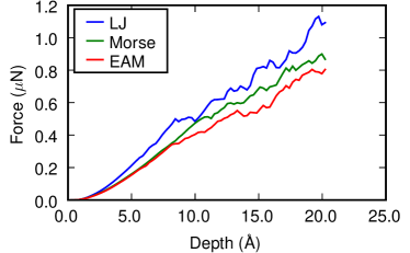
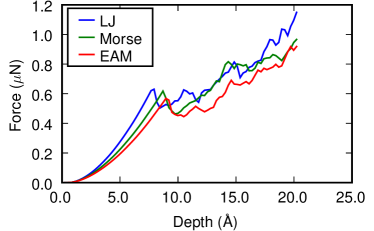
Figure 2: Force $F$ vs displacement $d$ for Cu. Crystal orientation: a) (100) b) (111).

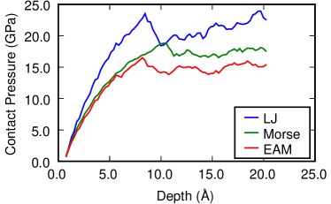
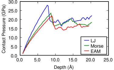
Figure 3: Contact pressure vs displacement $d$ for Cu. Crystal orientation: a) (100) b) (111).