Linear Time Encoding of LDPC Codes

Abstract

In this paper, we propose a linear complexity encoding method for arbitrary LDPC codes. We start from a simple graph-based encoding method “label-and-decide.” We prove that the “label-and-decide” method is applicable to Tanner graphs with a hierarchical structure—pseudo-trees— and that the resulting encoding complexity is linear with the code block length. Next, we define a second type of Tanner graphs—the encoding stopping set. The encoding stopping set is encoded in linear complexity by a revised label-and-decide algorithm—the ”label-decide-recompute.” Finally, we prove that any Tanner graph can be partitioned into encoding stopping sets and pseudo-trees. By encoding each encoding stopping set or pseudo-tree sequentially, we develop a linear complexity encoding method for general LDPC codes where the encoding complexity is proved to be less than $4\cdot M\cdot(\overline{k}-1)$, where $M$ is the number of independent rows in the parity check matrix and $\overline{k}$ represents the mean row weight of the parity check matrix.

I Introduction

Low Density Parity Check (LDPC) codes [1] are excellent error correcting codes with performance close to the Shannon Capacity [2]. The key weakness of LDPC codes is their apparently high encoding complexity. The conventional way to encode LDPC codes is to multiply the data words $\overrightarrow{s}$ by the code generator matrix $\mathbf{G}$, i.e., the code words are $\overrightarrow{x}=\mathbf{G}\cdot\overrightarrow{s}$. Though the parity-check matrix $\mathbf{H}$ for LDPC codes is sparse, the associated generator matrix $\mathbf{G}$ is not. The encoding complexity of LDPC codes is $\mathcal{O}(n^{2})$ where $n$ is the block length of the LDPC code. For moderate to high code block length $n$, this quadratic behavior is very significant and it severely affects the application of LDPC codes. For example, LDPC codes have advantages over turbo codes [3] in almost every aspect except that LDPC codes have $\mathcal{O}(n^{2})$ encoding complexity, while turbo codes have $\mathcal{O}(n)$ encoding complexity. It is highly desirable to reduce the $\mathcal{O}(n^{2})$ encoding complexity of LDPC codes.

Several authors have addressed the issue of speeding encoding of LDPC codes and, largely speaking, they follow three different paths. The first path designs efficient encoding methods for particular types of LDPC codes. We list a few typical representers. Reference [4] proposes a linear complexity encoding method for cycle codes—LDPC codes with column weight 2. Reference [5] presents an efficient encoder for quasi-cyclic LDPC codes. In [6], an efficient encoding approach is proposed for Reed-Solomon-type array codes. Reference [7] shows that there exists a linear time encoder for turbo-structured LDPC codes. Reference [8] constructs LDPC codes based on finite geometries and proves that this type of structured LDPC codes can be encoded in linear time. In [9, 11], two families of irregular LDPC Codes with cyclic structure and low encoding complexity are designed. In addition, an approximately lower triangular ensemble of LDPC Codes [10] was proposed to facilitate almost linear complexity encoding. The above low complexity encoders are only applicable to a small subset of LDPC codes, and some of the LDPC codes discussed above have performance loss when compared to randomly constructed LDPC codes. The second path borrows the decoder architecture and encodes LDPC codes iteratively on their Tanner graphs [12, 13]. The iterative LDPC encoding algorithm is easy to implement. However, there is no guarantee that iterative encoding will successfully get the codeword. In particular, the iterative encoding method will get trapped at the stopping set. The third path utilizes the sparseness of the parity check matrix to design a low complexity encoder. In [14], the authors present an algorithm named “greedy search” that reduces the coefficient of the quadratic term. This encoding method is relatively efficient. Its computation complexity and matrix storage need to be further reduced for most practical applications.

In this paper, we develop an exact linear complexity encoding method for arbitrary LDPC codes. We start from two particular Tanner graph structures—“pseudo-tree” and “encoding stopping set”— and prove that both the pseudo-tree and the encoding stopping set LDPC codes can be encoded in linear time. Next, we prove that any LDPC code with maximum column weight three can be decomposed into pseudo-trees and encoding stopping sets. Therefore, LDPC codes with maximum column weight three can be encoded in linear time and the encoding complexity is no more than $2\cdot M\cdot(\overline{k}-1)$ where $M$ denotes the number of independent rows of the parity check matrix and $\overline{k}$ represents the average row weight. Finally, we extend the $\mathcal{O}(n)$ complexity encoder to LDPC codes with arbitrary row weight distributions and column weight distributions. For arbitrary LDPC codes, we achieve $\mathcal{O}(n)$ encoding complexity, not exceeding $4\cdot M\cdot(\overline{k}-1)$.

The remaining of the paper is organized as follows. In Section II, we introduce relevant definitions and notation. Section III proposes a simple encoding algorithm “label-and-decide” that directly encodes an LDPC code on its Tanner graph. Section IV presents a particular type of Tanner graph with multi-layers—“pseudo-tree” and proves that any pseudo-tree can be encoded successfully in linear time by the label-and-decide algorithm. Section V studies the complement of the pseudo-tree—“encoding stopping set.” Section VI proves that the encoding stopping set can also be encoded in linear time by an encoding method named “label-decide-recompute.” Section VII demonstrates that any LDPC code with column weight at most three can be decomposed into pseudo-trees and encoding stopping sets. By encoding each pseudo-tree or encoding stopping set sequentially using the label-and-decide or the label-decide-recompute algorithms, we achieve linear complexity encoding for LDPC codes with maximum column weight three. Finally, we extend in this Section this linear time encoding method to LDPC codes with arbitrary column weight distributions and row weight distributions. Section VIII concludes the paper.

II Notation

LDPC codes. LDPC codes can be described by their parity-check matrix or their associated Tanner graph [15]. In the Tanner graph, each bit becomes a bit node and each parity-check constraint becomes a check node. If a bit is involved in a parity-check constraint, there is an edge connecting the bit node and the corresponding check node. The degree of a check node in a Tanner graph is equivalent to the number of one’s in the corresponding row of the parity check matrix, or, in another words, the row weight of the corresponding row. We will use the term “degree of a check node” and “row weight” interchangeably in this paper. Similarly, the degree of a bit node in a Tanner graph is equivalent to the column weight of the corresponding column of the parity check matrix, and we will interchangeably use the term “degree of a bit node” and “column weight” in this paper. The LDPC codes discussed in this paper may be irregular, i.e., different columns of the parity check matrix have different column weights and different rows of the parity check matrix have different row weights. The parity check matrix of an LDPC code may not be of full rank. If a row in the parity check matrix can be written as the binary sums of some other rows in the parity check matrix, this row is said to be dependent on the other rows. Otherwise, it is an independent row.

Arithmetic over the binary field. We represent by “$\oplus$” the summation over the binary field, i.e., an XOR operation. For example, $0\oplus 1=\mod(0+1\,,\,2)=1$. Similarly, we have $0\oplus 0=0$, $1\oplus 0=1$, $1\oplus 1=0$. In addition, we have the following equation $-x=x$ in the binary field.

Generalized parity check equation. A conventional parity check equation is shown in (1). The right-hand side of the parity check equation is always 0.

$$x_{1}\oplus x_{2}\oplus\ldots\oplus x_{k}=0$$ (1)

In this paper, we define the generalized parity check equation, as shown in (2)

$$x_{1}\oplus x_{2}\oplus\ldots\oplus x_{k}=b$$ (2)

On the right-hand side of equation (2), $b$ is a constant that can be either 0 or 1.

Let $C$ be a standard parity check equation. If the values of some of the bits in the left-hand side of $C$ are already known, then $C$ can be equivalently rewritten as a generalized parity check equation. For example, if the values of the bits $x_{p+1},x_{p+2},\ldots,x_{k}$ are known, we move these bits from the left-hand side of equation (1) to its right-hand side and rewrite it as follows.

$$x_{1}\oplus x_{2}\oplus\ldots\oplus x_{p}=x_{p+1}\oplus x_{p+2}\oplus\ldots\oplus x_{k}=b$$ (3)

Let $C_{1}$, $C_{2}$, $\ldots$, $C_{p}$ be $p$ generalized parity check equations, as shown in (4)

$$\begin{array}[]{c}\begin{array}[]{ccccccccc}C_{1}:&x_{1,1}&\oplus&x_{1,2}&\oplus&\ldots&x_{1,a_{1}}&=&b_{1}\\ C_{2}:&x_{2,1}&\oplus&x_{2,2}&\oplus&\ldots&x_{2,a_{2}}&=&b_{2}\\ \vdots&&\vdots&&&\vdots&&\vdots\\ C_{p}:&x_{p,1}&\oplus&x_{p,2}&\oplus&\ldots&x_{p,a_{p}}&=&b_{p}\end{array}\end{array}$$ (4)

We say $C_{1}$, $C_{2}$, $\ldots$, $C_{p}$ are dependent on each other if the corresponding homogeneous equations in (5) are dependent on each other.

$$\begin{array}[]{c}\begin{array}[]{ccccccccc}x_{1,1}&\oplus&x_{1,2}&\oplus&\ldots&x_{1,a_{1}}&=&0\\ x_{2,1}&\oplus&x_{2,2}&\oplus&\ldots&x_{2,a_{2}}&=&0\\ \vdots&&\vdots&&&\vdots&&\vdots\\ x_{p,1}&\oplus&x_{p,2}&\oplus&\ldots&x_{p,a_{p}}&=&0\end{array}\end{array}$$ (5)

From equations (4) and (5), we derive that

$$b_{1}\oplus b_{2}\oplus\ldots\oplus b_{p}=0$$ (6)

when the $p$ generalized parity check equations $C_{1}$, $C_{2}$, $\ldots$, $C_{p}$ are dependent on each other.

Connected graph. A graph is connected if there exists a path from any vertex to any other vertices in the graph. If a graph is not connected, we call it a disjoint graph.

Relative complement of a subgraph $\mathcal{S}$ in a Tanner graph $\mathcal{G}$. Let $\mathcal{G}$ be a Tanner graph and $\mathcal{S}$ be a subgraph of $\mathcal{G}$, i.e., $\mathcal{S}\subset\mathcal{G}$. We use the symbol $\mathcal{G}\backslash\mathcal{S}$ to denote the subgraph that contains the nodes and edges in $\mathcal{G}$, but not in $\mathcal{S}$. For example, let $C_{1}$, $C_{2}$, $\ldots$, $C_{k}$ be $k$ check nodes in a Tanner graph $\mathcal{G}$. The subgraph $\mathcal{G}\backslash\{C_{1},C_{2},\ldots,C_{k}\}$ represents the remaining graph after deleting check nodes $C_{1}$, $C_{2}$, $\ldots$, $C_{k}$ from $\mathcal{G}$. Assume $\mathcal{G}_{1}$, $\mathcal{G}_{2}$, $\ldots$, $\mathcal{G}_{k}$ are $k$ subgraphs in a Tanner graph $\mathcal{G}$. The notation $\mathcal{G}\backslash\{\mathcal{G}_{1}\cup\mathcal{G}_{2}\cup\ldots\cup\mathcal{G}_{k}\}$ represents the subgraph where nodes and edges are in $\mathcal{G}$, but not in $\mathcal{G}_{i}$, $1\leq i\leq k$.

III “Label-and-decide” Encoding Algorithm

Initially, Tanner graphs [15] were developed to explain the decoding process for LDPC codes; in fact, they can be used for the encoding of LDPC codes as well [12]. To encode an LDPC code using its Tanner graph, we identify information bits and parity bits through a labeling process on the graph. After determining the information bits and the parity bits, we start by assigning numerical values to the bit nodes labeled as information bits and then in a second step, calculate the missing values of the parity bits sequentially. This encoding approach is named label-and-decide. It is described in Algorithm 1.

Algorithm 1 Label-and-decide algorithm

  Preprocessing (carry out only once):

  Label every bit node either as information bit or parity bit on the Tanner graph.

  Encoding:

  $Flag\leftarrow 0$;

  Get the values of all the bits labeled as information bits;

  while there are parity bits undetermined do

     if there exists one undetermined parity bit $x$ that can be uniquely computed from the values of the information bits and the already determined parity bits then

        Compute the value of $x$.

     else

        $Flag\leftarrow 1$, exit the while loop.

     end if

  end while

  if $Flag=1$ then

     Encoding is unsuccessful.

  else

     Output the encoded codeword.

  end if

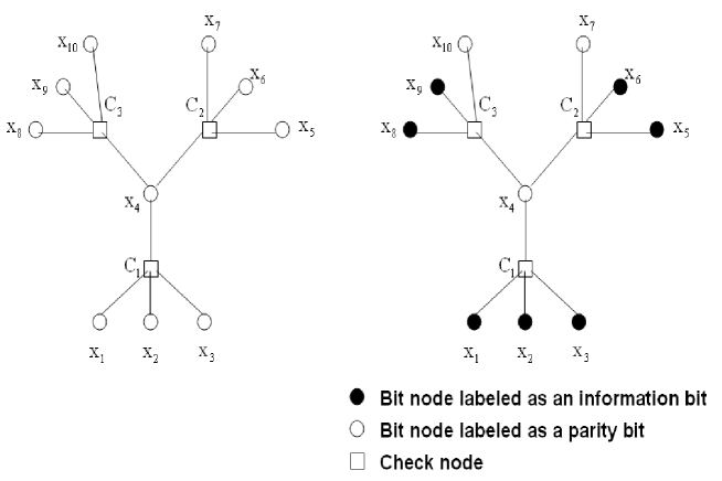
Figure 1: Left: A Tanner graph. Right: Labeling bit nodes on the Tanner graph shown on the left.

Example. Figure 1 shows on the left an LDPC code whose Tanner graph is a tree. Initially, all its bit nodes are unlabeled. First, we randomly pick bit nodes $x_{1}$, $x_{2}$, and $x_{3}$ to be information bits. According to the parity check equation $C_{1}$, the value of bit $x_{4}$ depends on the values of the bits $x_{1}$, $x_{2}$, and $x_{3}$ such that $x_{4}=x_{1}\oplus x_{2}\oplus x_{3}$. Therefore, $x_{4}$ should be labeled as a parity bit. Similarly, we label bits $x_{5}$, $x_{6}$, $x_{8}$, $x_{9}$ as information bits and label bits $x_{7}$, $x_{10}$ as parity bits. We represent information bits by solid circles and parity bits by empty circles. The labeling result is shown on the right in Figure 1.

By the above labeling process, we decide the systematic component of the code word $\overrightarrow{x}=(x_{1}\,\,x_{2}\,\,x_{3}\,\,x_{4}\,\,x_{5}\,\,x_{6}\,\,x_{7}\,\,x_{8}\,\,x_{9}\,\,x_{10})$ to be $\overrightarrow{s}=(x_{1}\,\,x_{2}\,\,x_{3}\,\,x_{5}\,\,x_{6}\,\,x_{8}\,\,x_{9})$ and the parity component to be $\overrightarrow{p}=(x_{4}\,\,x_{7}\,\,x_{10})$. The label-and-decide encoding on the code in Figure 1 then has the following steps:

• Get the values of the information bits $x_{1}$, $x_{2}$, $x_{3}$, $x_{5}$, $x_{6}$, $x_{8}$, and $x_{9}$ from the encoder input;

• Compute the parity bit $x_{4}$ from the parity check equation $C_{1}:x_{4}=x_{1}\oplus x_{2}\oplus x_{3}$;

• Compute the parity bit $x_{7}$ from the parity check equation $C_{2}$: $x_{7}=x_{4}\oplus x_{5}\oplus x_{6}$; compute the parity bit $x_{10}$ from the parity check equation $C_{3}$: $x_{10}=x_{4}\oplus x_{8}\oplus x_{9}$.

In fact, any tree code (whose Tanner graph is cycle-free) can be encoded in linear complexity by the label-and-decide algorithm. We will prove this fact in Corollary 2 in Section V. Further, the label-and-decide algorithm can be used to encode a particular type of Tanner graphs with cycles, i.e., the pseudo-tree we propose in the next section.

IV Pseudo-tree

A pseudo-tree is a connected Tanner graph that satisfies the following conditions (A1) through (A4).

• It is composed of $2P+1$ tiers where $P$ is a positive integer. We number these tiers from 1 to $2P+1$, starting from the top. The $(2i-1)$-th tier ($i=1,2,\ldots P+1$) contains only bit nodes, while the $(2i)$-th tier ($i=1,2,\ldots P$) contains only check nodes.

• Each bit node in the first tier has degree one and is connected to one and only one check node in the second tier.

• For each check node $C_{\alpha}$ in the $(2i)$-th tier, where $i$ can take any value from 1 to $P$, there is one and only one bit node $x_{\alpha}$ in the $(2i-1)$-th tier (immediate upper tier) that connects to $C_{\alpha}$, and there are no other bit nodes in the upper tiers that connect to $C_{\alpha}$. We call $x_{\alpha}$ the parent of $C_{\alpha}$ and $C_{\alpha}$ the child of $x_{\alpha}$.

• For each bit node $x_{\beta}$ in the $(2i-1)$-th tier, where $i$ can take any value from 2 to $P$, there is at most one check node $C_{\beta}$ in the $(2i)$-th tier (immediate lower tier) that connects to $x_{\beta}$, and there are no other check nodes in the lower tiers that connect to $x_{\beta}$.

For example, Figure 2 shows a pseudo-tree with seven tiers. It contains many cycles. Each check node $C_{i}$ in the pseudo-tree is connected to a unique bit node in the immediate upper tier, while each bit node $x_{i}$ in the pseudo-tree may connect to multiple check nodes in the upper tiers.

An important characteristic of a pseudo-tree is that it can be encoded in linear complexity by the label-and-decide algorithm. This is proved in the following lemma.

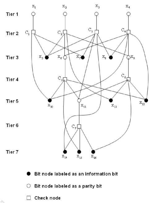
Figure 2: A pseudo-tree.

Lemma 1

Any LDPC code whose Tanner graph is a pseudo-tree is linear time encodable.

Proof: Let a pseudo-tree contain $2P+1$ tiers, $N$ bit nodes, and $M$ check nodes. Condition (A3) guarantees that each check node is connected to one and only one parent bit node in the immediate upper tier. Condition (A4) guarantees that different check nodes are connected to different parent bit nodes. Therefore, there are $M$ parent bit nodes for the check nodes. We label these $M$ parent bit nodes as parity bits and the other $N-M$ bit nodes as information bits.

The inputs of the encoder provide the values for all the information bits. The task of the encoder is to compute the values for all the parity bits. Let $x_{\alpha}$ be an arbitrary parity bit in the $(2i-1)$-th tier. By conditions (A3) and (A4), there is only one check node $C_{\alpha}$ in the lower tiers that connects to $x_{\alpha}$. The value of $x_{\alpha}$ is uniquely determined by the parity check equation represented by $C_{\alpha}$. According to condition (A3), all the bit nodes constrained by $C_{\alpha}$ except for $x_{\alpha}$ are in tiers below the $(2i-1)$-th tier. Therefore, the value of $x_{\alpha}$ depends only on the values of the bit nodes below the $(2i-1)$-th tier. For example, as shown in Figure 2, parity bit $x_{9}$ is the parent bit node of the check node $C_{6}$. From the parity check equation $C_{6}$, we see that the value of $x_{9}$ is computed from the values of $x_{11}$, $x_{12}$, $x_{16}$, and $x_{13}$, which are located below $x_{9}$. We compute the values of the parity bits tier by tier, starting from the $(2P-1)$-th tier (bottom tier) and then progressing upwards. Each time we compute the value of a parity bit, we only need the values of those bits (both information bits and parity bits) in lower tiers, which are already known. Hence, this encoding process can proceed. The encoding process is repeated until the values of all the parity bits in the first tier are known.

We evaluate the computation complexity of the above encoding process. Let $k_{i}$, $i=1,2,\dots,M$, denote the number of bits contained in the $i$-th parity check equation. The $i$-th parity check equation determines the value of a parity bit with $(k_{i}-2)$ XOR operations. So, $\sum_{i=1}^{M}(k_{i}-2)$ XOR operations are required to obtain all the $M$ parity bits. Let $\overline{k}=\frac{1}{M}\sum_{i=1}^{M}k_{i}$ denote the average number of bits in the $M$ parity check equations, then the encoding complexity is $\mathcal{O}(M(\overline{k}-2))$. For LDPC codes with uniform row weight $k$, the encoding complexity is $\mathcal{O}(M(k-2))$. The above analysis shows that the encoding process is accomplished in linear time. This completes the proof. $\Box$

We look at an example. We encode the pseudo-tree in Figure 2 as follows:

• Determine the values of all the information bits $x_{14}$, $x_{15}$, $x_{16}$, $x_{10}$, $x_{12}$, $x_{13}$, $x_{5}$, $x_{7}$, and $x_{8}$;

• Compute the parity bit $x_{11}$ from the parity check equation $C_{7}:x_{11}=x_{14}\oplus x_{15}\oplus x_{16}$;

• Compute the parity bit $x_{6}$ from the parity check equation $C_{5}:x_{6}=x_{10}\oplus x_{15}\oplus x_{11}\oplus x_{13}$; compute the parity bit $x_{9}$ from the parity check equation $C_{6}:x_{9}=x_{11}\oplus x_{12}\oplus x_{16}\oplus x_{13}$;

• Compute the parity bits $x_{1}$, $x_{2}$, $x_{3}$, and $x_{4}$ in the first tier by the parity check equations $C_{1}$, $C_{2}$, $C_{3}$, and $C_{4}$ respectively: $x_{1}=x_{10}\oplus x_{5}\oplus x_{7}$, $x_{2}=x_{5}\oplus x_{6}\oplus x_{12}\oplus x_{9}$, $x_{3}=x_{5}\oplus x_{7}\oplus x_{11}\oplus x_{14}\oplus x_{8}$, $x_{4}=x_{6}\oplus x_{8}\oplus x_{10}\oplus x_{9}\oplus x_{13}$.

The above encoding process requires only 21 XOR operations.

V Encoding Stopping Set

An encoding stopping set in a Tanner graph is a connected subgraph such that:

• If a check node $C$ is in an encoding stopping set, then all its associated bit nodes and the edges that are incident on $C$ are also in the encoding stopping set.

• Any bit node in an encoding stopping set is connected to at least two check nodes in the encoding stopping set.

• All the check nodes included in an encoding stopping set are independent of each other, i.e., any parity check equation can not be represented as the binary sums of other parity check equations.

The number of check nodes in an encoding stopping set is called its size. If a connected Tanner graph satisfies conditions (B1) and (B2) but not condition (B3), we call this Tanner graph a pseudo encoding stopping set. For example, the Tanner graph shown in Figure 3 is not an encoding stopping set but a pseudo encoding stopping set since it satisfies conditions (B1) and (B2) but not condition (B3). The Tanner graph shown in Figure 4 is an encoding stopping set. Its size is 9. Every bit node in this encoding stopping set has degree greater than or equal to 2, and every check node is independent of each other. Please note that the “encoding stopping set” defined in this paper is different from the “stopping set” defined in [16]. Stopping sets are used for the finite-length analysis of LDPC codes on the binary erasure channel, while encoding stopping sets are used here to develop efficient encoding methods for LDPC codes.

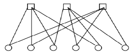
Figure 3: A pseudo encoding stopping set.

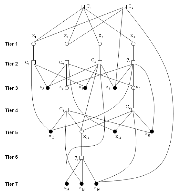
Figure 4: An encoding stopping set whose proper subgraph is a pseudo-tree shown in Figure 2.

From the above definitions of pseudo-tree and encoding stopping set, we have the following lemma.

Lemma 2

Any pseudo-tree or union of pseudo-trees does not contain encoding stopping sets.

The proof of Lemma 2 is straightforward. We omit it here.

We will show next that the label-and-decide algorithm can not successfully encode encoding stopping sets.

Theorem 1

An encoding stopping set can not be encoded successfully by the label-and-decide algorithm.

Proof: Let $\mathcal{E_{s}}$ be an encoding stopping set and suppose $\mathcal{E_{s}}$ can be encoded successfully by the label-and-decide algorithm. Let $x_{\alpha}$ be the last parity bit being determined during the encoding process. Since $\mathcal{E_{s}}$ is an encoding stopping set, $x_{\alpha}$ is connected to at least two check nodes $C_{\beta}$ and $C_{\gamma}$ by condition (B2). Further, by condition (B3), all the check nodes in $\mathcal{E_{s}}$, including $C_{\beta}$ and $C_{\gamma}$, are independent of each other. Hence, for certain encoder inputs, $C_{\beta}$ and $C_{\gamma}$ provide different values for the parity bit $x_{\alpha}$. This contradicts the fact that every parity bit can be uniquely determined successfully by the label-and-decide algorithm. Hence, the label-and-decide algorithm can not encode an encoding stopping set. This completes the proof. $\Box$

Conversely, if a Tanner graph does not contain any encoding stopping set, there must exist a linear complexity encoder for the corresponding code.

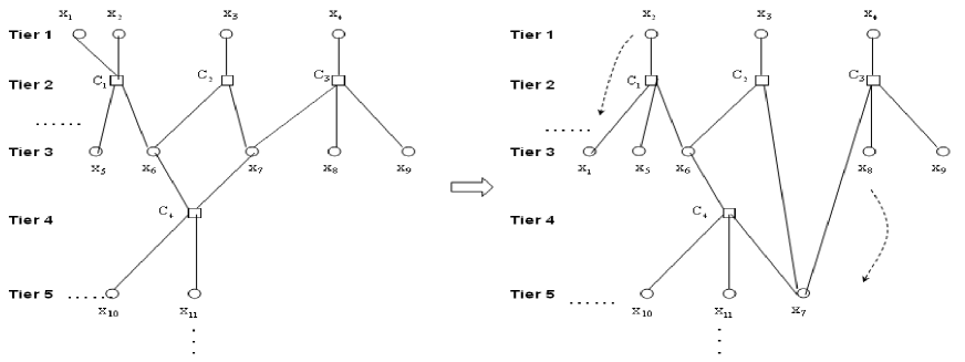
Figure 5: Left: A multi-layer structure but not a pseudo-tree. (Note that $C_{4}$ has two parents $x_{6}$ and $x_{7}$ and $C_{1}$ has two parents $x_{1}$ and $x_{2}$.) Right: The pseudo-tree that evolves from the multi-layer structure shown on the left.

Theorem 2

If a Tanner graph $\mathcal{G}$ does not contain any encoding stopping set, then it can be encoded in linear time by the label-and-decide algorithm.

Proof: We first delete all redundant check nodes (i.e., dependent on other check nodes) from the Tanner graph $\mathcal{G}$. Next, we restrict our attention to the case that $\mathcal{G}$ is a connected graph. We will show that $\mathcal{G}$ can be equivalently transformed into a pseudo-tree if it is free of any encoding stopping set. Since $\mathcal{G}$ does not contain any encoding stopping set, $\mathcal{G}$ itself is not an encoding stopping set. Hence, there exist some degree-one bit nodes in $\mathcal{G}$. We generate a multi-layer graph $\mathcal{T}$ and place those degree-one bit nodes in the first tier of $\mathcal{T}$. Next, the check nodes that connect to the degree-one bit nodes in the first tier of $\mathcal{T}$ are placed in the second tier of $\mathcal{T}$. Notice that there exist at least one bit node $x_{\alpha}$ in $\mathcal{G}\backslash\mathcal{T}$ such that $x_{\alpha}$ connects to at most one check node in $\mathcal{G}\backslash\mathcal{T}$. This statement is true. Otherwise, $\mathcal{G}\backslash\mathcal{T}$ becomes an encoding stopping set, which contradicts the fact that $\mathcal{G}$ does not contain any encoding stopping set. We pick all the bit nodes in $\mathcal{G}\backslash\mathcal{T}$ that connect to at most one check node in $\mathcal{G}\backslash\mathcal{T}$ and place them in the third tier of $\mathcal{T}$. Correspondingly, those check nodes in $\mathcal{G}\backslash\mathcal{T}$ that connect to the bit nodes in the third tier of $\mathcal{T}$ are placed in the fourth tier of $\mathcal{T}$. Each time we find bit nodes in $\mathcal{G}\backslash\mathcal{T}$ that connect to at most one check node in $\mathcal{G}\backslash\mathcal{T}$, we place those bit nodes in a new tier $2s+1$ of $\mathcal{T}$ and place the check nodes connecting to those bit nodes in the following new tier $2s+2$ of $\mathcal{T}$. We continue finding such bit nodes and increasing tiers till all the nodes in $\mathcal{G}$ are included in $\mathcal{T}$. Up to now, the multi-layer structure constructed so far satisfies the conditions (A1), (A2), and (A4). Condition (A3) may fail to be satisfied. For example, as shown on the left in Figure 5, the check node $C_{4}$ in tier 4 is connected to two bit nodes $x_{6}$ and $x_{7}$ in tier 3, which contradicts condition (A3). To satisfy condition (A3), we further adjust the positions of the bit nodes. If a check node in tier $2i$ is connected to $k$ bit nodes in the upper tiers of $\mathcal{T}$, we pick one bit node in tier $2i-1$ from these $k$ bit nodes and leave its position unchanged. Next, we drag the other $k-1$ bit nodes from their initial positions in tier $2i-1$ to the ($2i+1$)-th tier. To illustrate, let us focus on Figure 5 again. We drag the bit node $x_{7}$ from tier 3 to tier 5 and drag the bit node $x_{1}$ from tier 1 to tier 3. The newly formed graph is shown on the right in Figure 5, which follows condition (A3). By tuning the positions of the bit nodes in this way, the resulting hierarchical graph satisfies conditions (A1) to (A4). In this way, we transform $\mathcal{G}$ into a pseudo-tree. By Lemma 1, a pseudo-tree is linear time encodable. Therefore, the encoding complexity of $\mathcal{G}$ is $\mathcal{O}(M)$ where $M$ denotes the number of independent check nodes contained in $\mathcal{G}$.

We now prove the case that $\mathcal{G}$ is a disjoint graph. Let $\mathcal{G}$ contain $p$ connected subgraphs: $\mathcal{G}_{1},\mathcal{G}_{2},\ldots,\mathcal{G}_{p}$. By the above analysis, the complexity of encoding $\mathcal{G}_{i}$ is $\mathcal{O}(M_{i}),i=1,2,\ldots,p$, where $M_{i}$ denotes the number of independent check nodes contained in $\mathcal{G}_{i}$. Since $\mathcal{G}=\mathcal{G}_{1}\cup\mathcal{G}_{2}\cup\ldots\cup\mathcal{G}_{p}$, then the encoding complexity of $\mathcal{G}$ is $\sum_{i=1}^{p}\mathcal{O}(M_{i})=\mathcal{O}(\sum_{i=1}^{p}M_{i})=\mathcal{O}(M)$ where $M$ is the number of independent check nodes in $\mathcal{G}$. This completes the proof. $\Box$

From Theorem 2, we easily derive the following corollaries.

Corollary 1

If a Tanner graph does not contain any encoding stopping set, then it can be represented by a union of pseudo-trees.

The proof of Corollary 1 can be found in the proof of Theorem 2.

Corollary 2

The label-and-decide algorithm can encode any tree LDPC codes (whose Tanner graphs are cycle-free) with linear complexity.

Proof: Let $\mathcal{T}$ be the Tanner graph of a tree LDPC code and $\mathcal{S}$ be an arbitrary subgraph of $\mathcal{T}$. Since the Tanner graph $\mathcal{T}$ is a tree, its subgraph $\mathcal{S}$ is either a tree or a union of trees. Therefore, the graph $\mathcal{S}$ contains at least one bit leaf node with degree one. Since the graph $\mathcal{S}$ contains a degree-one bit node, $\mathcal{S}$ can not be an encoding stopping set. Since no subgraph of $T$ is an encoding stopping set, by Theorem 2, the tree code $\mathcal{T}$ can be encoded in linear complexity by the label-and-decide algorithm. This completes the proof. $\Box$

Corollary 3

A regular LDPC code with column weight 2 (cycle code) can be encoded in linear complexity by the label-and-decide algorithm.

Proof: We prove Corollary 3 by showing that a cycle code does not contain any encoding stopping set. Assume the cycle code contains an encoding stopping set $\mathcal{E_{s}}$. By the definition of cycle code and condition (B2), all the bit nodes in $\mathcal{E_{s}}$ have uniform degree two. It follows that the binary sum of all the parity check equations in $\mathcal{E_{s}}$ is a vector of 0’s. Then, at least one check node in $\mathcal{E_{s}}$ is dependent on the other check nodes. This contradicts condition (B3) that all the check nodes in an encoding stopping set are independent of each other. Hence, a cycle code does not contain any encoding stopping set. By Theorem 2, a cycle code is linear time encodable by the label-and-decide algorithm. This completes the proof. $\Box$

An alternative proof can be found in [4].

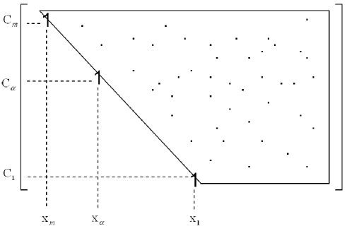
Figure 6: A parity check matrix in upper triangular form.

Corollary 4

Let $\bf H$ be the parity check matrix of an LDPC code. If $\bf H$ can be transformed into an upper triangular matrix $\bf U$ by row and column permutations, then the LDPC code can be encoded in linear time by the label-and-decide algorithm.

Proof: We label the rows of the upper triangular matrix $\bf U$ one by one as $C_{1}$, $C_{2}$, $\ldots$, $C_{m}$, from the bottom to the top, as shown in Figure 6. We notice that if $i>j$, then there exists at least one bit that is contained in $C_{i}$ but not in $C_{j}$. Assume the Tanner graph of the code contains an encoding stopping set $\mathcal{E_{s}}$ that contains check nodes $C_{i_{1}}$, $C_{i_{2}}$, $\ldots$, $C_{i_{p}}$. Let $q=\max(i_{1},i_{2},\ldots,i_{p})$. There exists at least one bit node $x_{q}$ in $\mathcal{E_{s}}$ that only connects to $C_{q}$. This contradicts the fact that every bit node in an encoding stopping set is connected to at least two check nodes in the encoding stopping set. Hence, $\mathcal{E_{s}}$ is not an encoding stopping set. Since the Tanner graph of the LDPC code does not contain any encoding stopping set, by Theorem 2 it is linear time encodable. This completes the proof. $\Box$

Theorems 1 and 2 show that encoding stopping sets prevent the application of the label-and-decide algorithm. However, we will show in the next section that encoding stopping sets can also be encoded in linear complexity.

VI Linear complexity encoding approach for encoding stopping sets

Let $\mathcal{E_{s}}$ be an encoding stopping set. We say $\mathcal{E_{s}}$ is a k-fold-constraint encoding stopping set if the following two conditions hold.

• There exist $k$ check nodes $C_{1}$, $C_{2}$, $\ldots$, $C_{k}$ in $\mathcal{E_{s}}$ such that $\mathcal{E_{s}}\backslash\{C_{1},C_{2},\ldots,C_{k}\}$ does not contain any encoding stopping set. We call the $k$ check nodes $C_{1}$, $C_{2}$, $\ldots$, $C_{k}$ key check nodes.

• For any $k-1$ check nodes $C_{1}$, $C_{2}$, $\ldots$, $C_{k-1}$ in $\mathcal{E_{s}}$, $\mathcal{E_{s}}\backslash\{C_{1},C_{2},\ldots,C_{k-1}\}$ contains an encoding stopping set.

The notation $\mathcal{E_{s}}\backslash\{C_{1},C_{2},\ldots,C_{k}\}$ denotes the remaining graph after deleting check nodes $C_{1}$, $C_{2}$, $\ldots$, $C_{k}$ from $\mathcal{E_{s}}$. Figure 4 shows a 2-fold-constraint encoding stopping set. After deleting the two key check nodes $C_{8}$ and $C_{9}$ from this encoding stopping set, the Tanner graph turns into a pseudo-tree, see Figure 2. We will focus on 1-fold-constraint and 2-fold-constraint encoding stopping sets in this paper, since we will show later that all types of LDPC codes can be decomposed into 1-fold or 2-fold constraint encoding stopping sets and pseudo-trees.

Let us first look at a 2-fold-constraint encoding stopping set $\mathcal{E_{s}}$ of size $M$. By definition, there exist two key check nodes $C_{\alpha}$ and $C_{\beta}$ in $\mathcal{E_{s}}$ such that $\mathcal{E_{s}}\backslash\{C_{\alpha},C_{\beta}\}$ does not contain any encoding stopping set. We encode $\mathcal{E_{s}}$ in three steps. In the first step, we encode $\mathcal{E_{s}}\backslash\{C_{\alpha},C_{\beta}\}$ using the label-and-decide algorithm according to Theorem 2. During encoding, $M-2$ bit nodes are labeled as parity bits and the remaining bit nodes are labeled as information bits. In the second step, we verify the two key check nodes $C_{\alpha}$ and $C_{\beta}$ based on the bit values acquired in Step 1. The key check nodes $C_{\alpha}$ and $C_{\beta}$ indicate that two bits $x_{\gamma}$ and $x_{\delta}$ that were previously labeled as information bits are actually parity bits, and their values are determined by $C_{\alpha}$ and $C_{\beta}$. We call the two bits $x_{\gamma}$ and $x_{\delta}$ reevaluated bits. The bits $x_{\gamma}$ and $x_{\delta}$ satisfy the following three conditions.

• $x_{\gamma}$ is constrained by the parity check equation $C_{\alpha}$.

• $x_{\delta}$ is constrained by the parity check equation $C_{\beta}$.

• $x_{\gamma}$ and $x_{\delta}$ are not both contained in $C_{\alpha}$ and $C_{\beta}$.

Since $C_{\alpha}$, $C_{\beta}$, and the other check nodes in $\mathcal{E_{s}}$ are independent of each other, there must exist bit nodes $x_{\gamma}$ and $x_{\delta}$ that satisfy conditions (D1) to (D3). An algorithm for finding reevaluated bits $x_{\gamma}$ and $x_{\delta}$ from a 2-fold-constraint encoding stopping set is presented in Appendix A. Notice that the work load to find the two key check nodes and the two reevaluated bits is a preprocessing step that is carried out only once. Assume in step 1 that $x_{\gamma}$ and $x_{\delta}$ are randomly assigned initial values $x_{\gamma}^{0}$ and $x_{\delta}^{0}$, respectively. If the parity check equations $C_{\alpha}$ and $C_{\beta}$ are both satisfied, the initial values $x_{\gamma}^{0}$ and $x_{\delta}^{0}$ are the correct values for $x_{\gamma}$ and $x_{\delta}$. If $C_{\alpha}$, or $C_{\beta}$, or both, are not satisfied, we need to recompute the values of $x_{\gamma}$ and $x_{\delta}$ from the values of the key check nodes $C_{\alpha}$ and $C_{\beta}$. Let $\triangle x_{\gamma}=\widetilde{x_{\gamma}}-x_{\gamma}^{0}$ and $\triangle x_{\delta}=\widetilde{x_{\delta}}-x_{\delta}^{0}$ where $\widetilde{x_{\gamma}}$ and $\widetilde{x_{\delta}}$ are the correct values of $x_{\gamma}$ and $x_{\delta}$, respectively, and let $\widetilde{C_{\alpha}}$ and $\widetilde{C_{\beta}}$ be the values of the key check nodes $C_{\alpha}$ and $C_{\beta}$, respectively. If $x_{\gamma}$ is contained in both $C_{\alpha}$ and $C_{\beta}$, and $x_{\delta}$ is only contained in $C_{\beta}$, we derive the following equations.

$$\begin{array}[]{c}\begin{array}[]{ccccc}\triangle x_{\gamma}&=&-\widetilde{C_{\alpha}}=\widetilde{C_{\alpha}}\\ \triangle x_{\gamma}\oplus\triangle x_{\delta}&=&-\widetilde{C_{\beta}}=\widetilde{C_{\beta}}\end{array}\end{array}$$ (7)

If $x_{\delta}$ is contained in both $C_{\alpha}$ and $C_{\beta}$, and $x_{\gamma}$ is only contained in $C_{\alpha}$, we derive the following equations.

$$\begin{array}[]{c}\begin{array}[]{ccccc}\triangle x_{\gamma}\oplus\triangle x_{\delta}&=&-\widetilde{C_{\alpha}}=\widetilde{C_{\alpha}}\\ \triangle x_{\delta}&=&-\widetilde{C_{\beta}}=\widetilde{C_{\beta}}\par\end{array}\end{array}$$ (8)

If $x_{\gamma}$ is only contained in $C_{\alpha}$ and $x_{\delta}$ is only contained in $C_{\beta}$, we have the following equations.

$$\begin{array}[]{c}\begin{array}[]{ccccc}\triangle x_{\gamma}&=&-\widetilde{C_{\alpha}}=\widetilde{C_{\alpha}}\\ \triangle x_{\delta}&=&-\widetilde{C_{\beta}}=\widetilde{C_{\beta}}\par\end{array}\end{array}$$ (9)

From equations (7) to (9), we can get the correct values of $x_{\gamma}$ and $x_{\delta}$. In the third step, we recompute those parity bits that are affected by the new values of $x_{\gamma}$ and $x_{\delta}$. This encoding method is named label-decide-recompute and is described in Algorithm 2.

Algorithm 2 Label-decide-recompute algorithm for a 2-fold-constraint encoding stopping set $\mathcal{E_{s}}$ of size $M$

  Preprocessing (carry out only once):

  Find two check nodes $C_{\alpha}$ and $C_{\beta}$ such that $\mathcal{E_{s}}\backslash\{C_{\alpha},C_{\beta}\}$ does not contain any encoding stopping set;

  Using Algorithm 8 to pick two information bits $x_{\gamma}$ and $x_{\delta}$ that satisfy conditions (D1) to (D3).

  Determine the parity bits $x_{p_{1}}$, $x_{p_{2}}$, $\ldots$, $x_{p_{s}}$ that are affected by the values of $x_{\gamma}$ and $x_{\delta}$;

  Encoding:

  Fill the values of the information bits except for $x_{\gamma}$ and $x_{\delta}$;

  Assign $x_{\gamma}=0$ and $x_{\delta}=0$;

  Encode $\mathcal{E_{s}}\backslash\{C_{\alpha},C_{\beta}\}$ using Algorithm 1. Compute the values of the $M-2$ parity bits;

  Compute the values $\widetilde{C_{\alpha}}$ and $\widetilde{C_{\beta}}$ of the key check nodes $C_{\alpha}$ and $C_{\beta}$, respectively;

  if $\widetilde{C_{\alpha}}\neq 0$ or $\widetilde{C_{\beta}}\neq 0$ then

     Recompute the values of $x_{\gamma}$ and $x_{\delta}$ from $\widetilde{C_{\alpha}}$ and $\widetilde{C_{\beta}}$ by equations (7) to (9);

     for $i$ = 1 to $s$ do

        Recompute the value of the parity bit $x_{p_{i}}$ based on the new values of $x_{\gamma}$ and $x_{\delta}$;

     end for

  end if

  Output the encoding result.

Next, we analyze the computation complexity of the label-decide-recompute algorithm when encoding a 2-fold-constraint encoding stopping set. Every check node except for the two key check nodes $C_{\alpha}$ and $C_{\beta}$ are computed at most twice in the label-decide-recompute encoding (label-and-decide step and recompute step) while the two key check nodes $C_{\alpha}$ and $C_{\beta}$ need to be computed only once. In addition, we need one extra XOR operation to compute the two reevaluated bits $x_{\gamma}$ and $x_{\delta}$ by equations (7) to (9). Hence, the encoding complexity of the label-decide-recompute algorithm is less than or equal to $2\cdot\sum_{i=1}^{M-2}(k_{i}-2)+(k_{\alpha}-1)+(k_{\beta}-1)+1$ where $k_{i}$, $1\leq i\leq M-2$, are the degrees of the check nodes other than $C_{\alpha}$, $C_{\beta}$ and $k_{\alpha}$, $k_{\beta}$ are the degrees of the check nodes $C_{\alpha}$ and $C_{\beta}$, respectively. The encoding complexity of the label-decide-recompute algorithm can be further simplified to be less than $2\cdot M\cdot(\overline{k}-1)$ where $M$ is the number of check nodes in the encoding stopping set and $\overline{k}$ is the average number of bit nodes contained in each check node in the encoding stopping set. This shows that the label-decide-recompute algorithm encodes any 2-fold-constraint encoding stopping set in linear time. The pre-processing (determining key check nodes, reevaluated bits, and parity bits affected by the reevaluated bits) is done offline and does not count towards encoder complexity.

We look at an example. Figure 4 shows a 2-fold-constraint encoding stopping set $\mathcal{E_{s}}$. After deleting the two check nodes $C_{8}$ and $C_{9}$, $\mathcal{E_{s}}$ becomes the pseudo-tree shown in Figure 2. In addition, the value of the bit node $x_{5}$ affects $C_{8}$ and the value of the bit node $x_{8}$ affects $C_{9}$. Hence, the two bits $x_{5}$ and $x_{8}$ are reevaluated bits. We use the label-decide-recompute algorithm to encode $\mathcal{E_{s}}$ as follows.

• Assign $x_{5}=0$ and $x_{8}=0$. Encode the pseudo-tree part following the procedures on page 10.

• Compute the values of the key check nodes $C_{8}$ and $C_{9}$, e.g., $\widetilde{C_{8}}=x_{1}\oplus x_{2}\oplus x_{3}\oplus x_{4}$ and $\widetilde{C_{9}}=x_{1}\oplus x_{2}\oplus x_{8}\oplus x_{16}$.

  • If $\widetilde{C_{8}}=0$ and $\widetilde{C_{9}}=0$, stop encoding and output the codeword $[x_{1}\,\,x_{2}\,\,\ldots\,\,x_{16}]$.

  • If $\widetilde{C_{8}}=1$ or $\widetilde{C_{9}}=1$, recompute the values of $x_{5}$ and $x_{8}$ as follows: $x_{5}=\widetilde{C_{8}}$ and $x_{8}=\widetilde{C_{9}}$, where $\widetilde{C_{8}}$ and $\widetilde{C_{9}}$ are the values of the parity check equations $C_{8}$ and $C_{9}$, respectively. Recompute the parity bits $x_{1}$, $x_{2}$, $x_{3}$, and $x_{4}$ based on the new values of $x_{5}$ and $x_{8}$. Output the codeword $[x_{1}\,\,x_{2}\,\,\ldots\,\,x_{16}]$.

The label-decide-recompute algorithm can be further simplified. We restudy the third step of the label-decide-recompute method. Assume $p_{1}$, $p_{2}$, $\ldots$, $p_{m}$ are the parity bits whose values need to be updated. In order to get the new values of the parity bits $p_{1}$, $p_{2}$, $\ldots$, $p_{m}$, we need to recompute those parity check equations that relate to $p_{1}$, $p_{2}$, $\ldots$, $p_{m}$. In fact, instead of recomputing the parity check equations relating to $p_{1}$, $p_{2}$, $\ldots$, $p_{m}$, we can directly flip the values of the parity bits $p_{1}$, $p_{2}$, $\ldots$, $p_{m}$ since in the binary field the value of a bit is either 0 or 1. For example, if the correct value of $x_{\gamma}$ is different from its original value $x_{\gamma}^{0}$, we simply flip the values of those parity bits that are affected by $x_{\gamma}$. We name the above encoding method label-decide-flip and describe it in Algorithm 3. The encoding complexity of Algorithm 3 is $M\cdot(\overline{k}-1)$ XOR operations plus two vector flipping operations.

Algorithm 3 Label-decide-flip algorithm for a 2-fold-constraint encoding stopping set $\mathcal{E_{s}}$ of size $M$

  Preprocessing (carry out only once):

  Find two check nodes $C_{\alpha}$ and $C_{\beta}$ such that $\mathcal{E_{s}}\backslash\{C_{\alpha},C_{\beta}\}$ does not contain any encoding stopping set;

  Using Algorithm 8 to pick two information bits $x_{\gamma}$ and $x_{\delta}$ that satisfy conditions (D1) to (D3).

  Determine the parity bits $x_{u_{1}}$, $x_{u_{2}}$, $\ldots$, $x_{u_{r}}$ that are affected by the value of $x_{\gamma}$ and group $x_{u_{1}}$, $x_{u_{2}}$, $\ldots$, $x_{u_{r}}$ in a vector $\overrightarrow{X_{\gamma}}=[x_{u_{1}}\,\,x_{u_{2}}\,\,\ldots\,\,x_{u_{r}}]$. Determine the parity bits $x_{p_{1}}$, $x_{p_{2}}$, $\ldots$, $x_{p_{s}}$ that are affected by the value of $x_{\delta}$ and group $x_{p_{1}}$, $x_{p_{2}}$, $\ldots$, $x_{p_{s}}$ in a vector $\overrightarrow{X_{\delta}}=[x_{p_{1}}\,\,x_{p_{2}}\,\,\ldots\,\,x_{p_{s}}]$. Determine the parity bits $x_{q_{1}}$, $x_{q_{2}}$, $\ldots$, $x_{q_{t}}$ that are affected by the value of $x_{\gamma}\oplus x_{\delta}$ and group $x_{q_{1}}$, $x_{q_{2}}$, $\ldots$, $x_{q_{t}}$ in a vector $\overrightarrow{X_{\epsilon}}=[x_{q_{1}}\,\,x_{q_{2}}\,\,\ldots\,\,x_{q_{t}}]$.

  Encoding:

  Fill the values of the information bits except for $x_{\gamma}$ and $x_{\delta}$;

  Assign $x_{\gamma}=0$ and $x_{\delta}=0$;

  Encode $\mathcal{E_{s}}\backslash\{C_{\alpha},C_{\beta}\}$ using Algorithm 1. Compute the values of the $M-2$ parity bits;

  Compute the values $\widetilde{C_{\alpha}}$ and $\widetilde{C_{\beta}}$ of the parity check equations $C_{\alpha}$ and $C_{\beta}$, respectively;

  if $\widetilde{C_{\alpha}}\neq 0$ or $\widetilde{C_{\beta}}\neq 0$ then

     Recompute the values of $x_{\gamma}$ and $x_{\delta}$ from $\widetilde{C_{\alpha}}$ and $\widetilde{C_{\beta}}$ by equations (7) to (9);

     if $x_{\gamma}=1$ then

        Flip the vector $\overrightarrow{X_{\gamma}}$.

     end if

     if $x_{\delta}=1$ then

        Flip the vector $\overrightarrow{X_{\delta}}$.

     end if

     if $x_{\gamma}\oplus x_{\delta}=1$ then

        Flip the vector $\overrightarrow{X_{\epsilon}}$.

     end if

  end if

  Output the encoding result.

We, again, look at an example. The 2-fold-constraint encoding stopping set shown in Figure 4 can be encoded by Algorithm 3 as follows.

• Assign $x_{5}=0$ and $x_{8}=0$. Encode the pseudo-tree part following the procedures on page 10.

• Compute the values of the parity check equations $C_{8}$ and $C_{9}$, e.g., $\widetilde{C_{8}}=x_{1}\oplus x_{2}\oplus x_{3}\oplus x_{4}$ and $\widetilde{C_{9}}=x_{1}\oplus x_{2}\oplus x_{8}\oplus x_{16}$.

  • If $\widetilde{C_{8}}=0$ and $\widetilde{C_{9}}=0$, stop encoding and output the codeword $[x_{1}\,\,x_{2}\,\,\ldots\,\,x_{16}]$.

  • If $\widetilde{C_{8}}=1$ or $\widetilde{C_{9}}=1$, recompute the values of $x_{5}$ and $x_{8}$ as the following: $x_{5}=\widetilde{C_{8}}$ and $x_{8}=\widetilde{C_{9}}$ where $\widetilde{C_{8}}$ and $\widetilde{C_{9}}$ are the values of the parity check equations $C_{8}$ and $C_{9}$, respectively. If $x_{5}=1$, flip the vector $[x_{1}\,\,x_{2}\,\,x_{3}]$ to be $[\sim x_{1}\,\,\sim x_{2}\,\,\sim x_{3}]$. If $x_{8}=1$, flip the vector $[x_{3}\,\,x_{4}]$. If $x_{5}\oplus x_{8}=1$, flip the vector $[x_{4}]$. Output the codeword $[x_{1}\,\,x_{2}\,\,\ldots\,\,x_{16}]$.

It is easy to revise Algorithm 2 and Algorithm 3 to encode a 1-fold-constraint encoding stopping set. For example, Algorithm 4 shows the label-decide-recompute algorithm for a 1-fold-constraint encoding stopping set. The encoding complexity of Algorithm 4 is less than $2\cdot M\cdot(\overline{k}-1)$ where $M$ is the number of check nodes in the encoding stopping set and $\overline{k}$ is the average number of bit nodes contained in each check node in the encoding stopping set.

Algorithm 4 Label-decide-recompute algorithm for a 1-fold-constraint encoding stopping set $\mathcal{E_{s}}$ of size $M$

  Preprocessing (carry out only once):

  Find a check node $C^{*}$ such that $\mathcal{E_{s}}\backslash C^{*}$ does not contain any encoding stopping set.

  Pick an information bit $x^{*}$ that is constrained by the parity check equation $C^{*}$.

  Determine the parity bits $x_{p_{1}}$, $x_{p_{2}}$, $\ldots$, $x_{p_{s}}$ that are affected by $x^{*}$.

  Encoding:

  Fill the values of the information bits except for $x^{*}$.

  Assign $x^{*}=0$.

  Encode $\mathcal{E_{s}}\backslash C^{*}$ using Algorithm 1, compute the values of the $M-1$ parity bits.

  Verify the parity check equation $C^{*}$.

  if the parity check equation $C^{*}$ is not satisfied then

     $x^{*}\leftarrow 1$.

     for $i$ = 1 to s do

        Recompute the value of the parity bit $x_{p_{i}}$ based on the new value of $x^{*}$;

     end for

  end if

  Output the encoding result.

VII Linear complexity encoding for general LDPC codes

In this section, we propose a linear complexity encoding method for general LDPC codes. We will show that any Tanner graph can be decomposed into pseudo-trees and encoding stopping sets that are 1-fold-constraint or 2-fold-constraint. By encoding each pseudo-tree or encoding stopping set using Algorithm 1 or Algorithm 2, we achieve linear time encoding for arbitrary LDPC codes.

To proceed, we provide the following definition. Given a Tanner graph $\mathcal{G}$ and its subgraph $\mathcal{S}$, we call the bit nodes in $\mathcal{G}$ but not in $\mathcal{S}$ the outsider nodes of $\mathcal{S}$. For example, Figure 7 shows a Tanner graph $\mathcal{G}$ and its subgraph $\mathcal{S}$. Since in Figure 7 the two bit nodes $x_{1}$ and $x_{2}$ are in $\mathcal{G}$ but not in $\mathcal{S}$, $x_{1}$ and $x_{2}$ are outsider nodes of $\mathcal{S}$. The check node $C_{2}$ contains two outsider nodes of $\mathcal{S}$, i.e., is connected to two outsider nodes. The check node $C_{1}$ contains zero outsider nodes of $\mathcal{S}$.

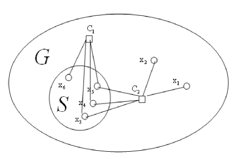
Figure 7: Outsider nodes.

We start from LDPC codes with maximum column weight 3 by proving the following lemma.

Lemma 3

Assume the maximum bit node degree of a Tanner graph $\mathcal{G}$ is three, then one of the following statements must be true.

• There are no pseudo encoding stopping sets or encoding stopping sets in $\mathcal{G}$.

• There exists a pseudo encoding stopping set in $\mathcal{G}$. All the bit nodes in the pseudo encoding stopping set have uniform degree 2.

• There exists a 1-fold-constraint or a 2-fold-constraint encoding stopping set in $\mathcal{G}$.

Proof: We only need to prove either condition (E2), or condition (E3), is true if $\mathcal{G}$ contains a pseudo encoding stopping set, or an encoding stopping set, respectively. We prove this statement by constructing a subgraph $\mathcal{S}$ from the Tanner graph $\mathcal{G}$. Initially $\mathcal{S}$ is empty. We pick a check node $C_{1}$ from $\mathcal{G}$ that contains the smallest number of bit nodes. Next, we add $C_{1}$ and all the bit nodes contained in $C_{1}$ to $\mathcal{S}$. We keep adding check nodes and their associated bit nodes to $\mathcal{S}$ till $\mathcal{S}$ contains a pseudo encoding stopping set or an encoding stopping set. Each time we add a check node to $\mathcal{S}$, we always pick the check node that contains the fewest outsider nodes of $\mathcal{S}$. If $\mathcal{S}$ contains an encoding stopping set, we also add all the check nodes in $\mathcal{G}\backslash\mathcal{S}$ that contain zero outsider nodes to $\mathcal{S}$. Next, we discuss two different cases.

$\mathcal{S}$ contains an encoding stopping set. Assume $\mathcal{S}$ contains $k$ check nodes and the $j$-th added check node $C_{j}$ is the last check node that introduces outsider nodes to $\mathcal{S}$. We will show that $k-j\leq 2$. Assume $C_{j}$ adds $p$ outsider nodes $x_{j_{1}}$, $x_{j_{2}}$, $\ldots$, $x_{j_{p}}$ to $\mathcal{S}$. We will prove that the $(j+1)$-th added check node $C_{j+1}$ connects to all the $p$ bit nodes $x_{j_{1}}$, $x_{j_{2}}$, $\ldots$, $x_{j_{p}}$. If $C_{j+1}$ does not connect to all the $p$ bit nodes, then $C_{j+1}$ contains a smaller number of outsider nodes than $C_{j}$ and should be added earlier than $C_{j}$ since we always pick the check node that contains the smallest number of outsider nodes and add it first to $\mathcal{S}$. This contradicts the fact that $C_{j+1}$ is added to $\mathcal{S}$ after $C_{j}$. Therefore, $C_{j+1}$ should connect to all the $p$ bit nodes $x_{j_{1}}$, $x_{j_{2}}$, $\ldots$, $x_{j_{p}}$. Similarly, $C_{j+2}$, $\ldots$, $C_{k}$ connect to all the $p$ bit nodes $x_{j_{1}}$, $x_{j_{2}}$, $\ldots$, $x_{j_{p}}$. Since any bit node can connect to at most three check nodes, it follows that $k-j\leq 2$, which means at most two check nodes are added to $\mathcal{S}$ after $C_{j}$. Notice that $\mathcal{S}$ does not contain any encoding stopping set before adding $C_{j+1}$. Hence, the encoding stopping set in $\mathcal{S}$ is either a 1-fold-constraint encoding stopping set or a 2-fold-constraint encoding stopping set. Condition (E2) is satisfied.

$\mathcal{S}$ is a pseudo encoding stopping set. It follows that the binary sum of all the check nodes in $\mathcal{S}$ is zero. So, the degree of every bit node in $\mathcal{S}$ is an even number. Since the maximum bit node degree is three, the degree of each bit node in $\mathcal{S}$ is two. Condition (E3) is satisfied.

This completes the proof. $\Box$

We detail the method of determining a pseudo encoding stopping set or an encoding stopping set in Algorithm 5.

Algorithm 5 Find a pseudo encoding stopping set or an encoding stopping set (1-fold-constraint or 2-fold-constraint) from a Tanner graph $\mathcal{G}$ with maximum bit node degree 3.

  $\mathcal{S}=\phi$.

  $Flag\leftarrow 0$.

  $i=1$.

  while $Flag=0$ and $\mathcal{G}\neq\mathcal{S}$ do

     Find a check node $C_{i}$ in $\mathcal{G}\backslash\mathcal{S}$ that contains the smallest number of outsider nodes of $\mathcal{S}$.

     Add $C_{i}$ and all its associated outsider nodes to $\mathcal{S}$.

     if $C_{i}$ does not introduce new bit nodes to $\mathcal{S}$ then

        $\mathcal{A}\leftarrow\mathcal{S}$.

        while there exists a bit node $x$ of degree one in $\mathcal{A}$ do

           Delete the degree-one bit node $x$ and the check node connecting to $x$ from $\mathcal{A}$.

        end while

        if $\mathcal{A}=\phi$ then

           $\mathcal{S}$ does not contain any pseudo encoding stopping set or encoding stopping set.

        else

           $Flag\leftarrow 1$.

        end if

     end if

     $i=i+1$.

  end while

  if $Flag=1$ then

     if all the bit nodes in $\mathcal{A}$ are of degree 2 then

        The subgraph $\mathcal{A}$ is a pseudo encoding stopping set.

     else

        The subgraph $\mathcal{A}$ is an encoding stopping set.

     end if

     Output $\mathcal{A}$.

  else

     The Tanner graph $\mathcal{G}$ does not contain pseudo encoding stopping sets or encoding stopping sets.

  end if

Theorem 3

Let $\mathcal{G}$ be the Tanner graph of an LDPC code. If the maximum bit node degree of $\mathcal{G}$ is three, then the LDPC code can be encoded in linear time and the encoding complexity is less than $2\cdot M\cdot(\overline{k}-1)$ where $M$ is the number of independent check nodes in $\mathcal{G}$ and $\overline{k}$ is the average number of bit nodes contained in each check node.

Proof: If the Tanner graph $\mathcal{G}$ does not contain any encoding stopping set, then the corresponding LDPC code can be encoded in linear time by Theorem 2. Therefore, we only need to prove Theorem 3 for the case that $\mathcal{G}$ contains encoding stopping sets. Since the maximum bit node degree of $\mathcal{G}$ is three, by Lemma 3 there exists a pseudo encoding stopping set or an encoding stopping set $\mathcal{G}_{1}$ in $\mathcal{G}$. If $\mathcal{G}_{1}$ is a pseudo encoding stopping set, we simply delete a redundant check node from $\mathcal{G}_{1}$ and $\mathcal{G}_{1}$ becomes a pseudo-tree. If $\mathcal{G}_{1}$ is an encoding stopping set, it is either a 1-fold-constraint or a 2-fold-constraint encoding stopping set by Lemma 3.

Next, we look at the subgraph $\mathcal{G}\backslash\mathcal{G}_{1}$. We first transform the parity check equations in $\mathcal{G}\backslash\mathcal{G}_{1}$ into generalized parity check equations by moving the bits contained in $\mathcal{G}_{1}$ from the left-hand side of the equation to the right-hand side of the equation. Let a parity check equation $C$ contain $k$ bit nodes $x_{1}$, $x_{2}$, $\ldots$, $x_{k}$ where the bits $x_{q+1}$, $\ldots$, $x_{k}$ are also in $\mathcal{G}_{1}$, then the parity check equation $C$ can be rewritten as

$$x_{1}\oplus x_{2}\oplus\ldots\oplus x_{k}=0\Longrightarrow x_{1}\oplus x_{2}\oplus\ldots\oplus x_{q}=x_{q+1}\oplus x_{q+2}\oplus\ldots\oplus x_{k}=b$$ (10)

In equation (10), $b$ becomes a constant after we encode $\mathcal{G}_{1}$ and get the values of all the bits in $\mathcal{G}_{1}$. Since the maximum bit node degree of $\mathcal{G}\backslash\mathcal{G}_{1}$ is less than or equal to three, we, again, find a pseudo encoding stopping set or an encoding stopping set $\mathcal{G}_{2}$ from $\mathcal{G}\backslash\mathcal{G}_{1}$. If $\mathcal{G}_{2}$ is an encoding stopping set, $\mathcal{G}_{2}$ is either a 1-fold-constraint or a 2-fold-constraint encoding stopping set by Lemma 3. If $\mathcal{G}_{2}$ is a pseudo encoding stopping set and we assume $\mathcal{G}_{2}$ contains the following $m$ generalized parity check equations,

$$\begin{array}[]{c}\begin{array}[]{ccccccccc}x_{1,1}&\oplus&x_{1,2}&\oplus&\ldots&x_{1,a_{1}}&=&b_{1}\\ x_{2,1}&\oplus&x_{2,2}&\oplus&\ldots&x_{2,a_{2}}&=&b_{2}\\ \vdots&&\vdots&&&\vdots&&\vdots\\ x_{m,1}&\oplus&x_{m,2}&\oplus&\ldots&x_{m,a_{m}}&=&b_{m}\end{array}\end{array}$$ (11)

we derive that

$$b_{1}\oplus b_{2}\oplus\ldots\oplus b_{m}=0$$ (12)

Hence, we can replace any generalized parity check equation in (11) by the new parity check equation (12). From the above analysis, we can delete any check node from $\mathcal{G}_{2}$ to make $\mathcal{G}_{2}$ a pseudo-tree. To maintain the code structure, we also generate a new check node $C^{*}$ that represents the parity check equation (12). Since the parity check equation (12) only contains bits in $\mathcal{G}_{1}$, we add the new check node $C^{*}$ to $\mathcal{G}_{1}$ and regenerate encoding stopping sets or pseudo-trees in the graph $\mathcal{G}_{1}\cup C^{*}$.

Generally, we can find a pseudo encoding stopping set or an encoding stopping set $\mathcal{G}_{i+1}$ from the subgraph $\mathcal{G}\backslash\{\mathcal{G}_{1}\cup\mathcal{G}_{2}\cup\ldots\cup\mathcal{G}_{i}\}$. If $\mathcal{G}_{i+1}$ is an encoding stopping set, $\mathcal{G}_{i+1}$ is either a 1-fold-constraint or a 2-fold-constraint encoding stopping set by Lemma 3. If $\mathcal{G}_{i+1}$ is a pseudo encoding stopping set, we operate in three steps. In the first step, we sum up all the generalized parity check equations in $\mathcal{G}_{i+1}$ to generate a new parity check equation $C^{*}$. In the second step, we delete one check node from $\mathcal{G}_{i+1}$ to make $\mathcal{G}_{i+1}$ a pseudo-tree. In the third step, we add the new check node $C^{*}$ to $\mathcal{G}_{i}$ and regenerate pseudo-tree or encoding stopping sets in $\mathcal{G}_{i}\cup C^{*}$. Notice that the new parity check equation $C^{*}$ in (12) does not incur extra cost to compute variables $b_{1}$, $b_{2}$, $\ldots$, $b_{m}$ since these variables have already been computed in those generalized parity check equations in $\mathcal{G}_{i+1}$, as shown in (11). Practically, we can compute these variables $b_{1}$, $b_{2}$, $\ldots$, $b_{m}$ only once and store them. Later, we can apply the stored values $b_{1}$, $b_{2}$, $\ldots$, $b_{m}$ to both equation (12) and equation (11). Hence, the new parity check equation $C^{*}$ only needs $m-1$ additional XOR operations to compute the summation of $b_{1}$, $b_{2}$, $\ldots$, $b_{m}$. Since the cost of encoding the pseudo-tree $\mathcal{G}_{i+1}$ is $(m-1)\cdot(\overline{k}-2)$ where $\overline{k}$ is the average degree of the remaining $m-1$ check nodes in $\mathcal{G}_{i+1}$, the overall cost of encoding $\mathcal{G}_{i+1}$ and the new parity check equation $C^{*}$ is $(m-1)\cdot(\overline{k}-1)$.

By continuing to find pseudo-tree or encoding stopping sets in this way, we reach the stage where $\mathcal{G}\backslash\{\mathcal{G}_{1}\cup\mathcal{G}_{2}\cup\ldots\cup\mathcal{G}_{i}\}=\phi$ or $\mathcal{G}\backslash\{\mathcal{G}_{1}\cup\mathcal{G}_{2}\cup\ldots\cup\mathcal{G}_{i}\}$ does not contain pseudo encoding stopping sets or encoding stopping sets.

By the above analysis, we decompose the Tanner graph $\mathcal{G}$ into a sequence of $p$ subgraphs $\mathcal{G}_{1}$, $\mathcal{G}_{2}$, $\ldots$, $\mathcal{G}_{p}$ where $\mathcal{G}_{i}$, $1\leq i\leq p$, is either a 1-fold-constraint encoding stopping set, a 2-fold-constraint encoding stopping set, or a pseudo-tree. If $\mathcal{G}_{i}$ is a 1-fold-constraint or a 2-fold-constraint encoding stopping set, we apply Algorithm 2 or Algorithm 4 to encode $\mathcal{G}_{i}$ and the resulting encoding complexity is less than $2\cdot M_{i}\cdot(\overline{k_{i}}-1)$ where $M_{i}$ denotes the number of independent check nodes in $\mathcal{G}_{i}$ and $\overline{k_{i}}$ denotes the average number of bit nodes contained in each check node in $\mathcal{G}_{i}$. If $\mathcal{G}_{i}$ is a pseudo-tree, we apply Algorithm 1 to encode $\mathcal{G}_{i}$ and the corresponding encoding complexity is less than $M_{i}\cdot(\overline{k_{i}}-1)$. The overall computation complexity of encoding $\mathcal{G}$ is linear on the number of independent check nodes $M$ in $\mathcal{G}$ and is bounded by $\sum_{i=1}^{p}(2\cdot M_{i}\cdot(\overline{k_{i}}-1))=2\cdot M\cdot(\overline{k}-1)$ where $\overline{k}$ denotes the average number of bits contained in each independent check node of $\mathcal{G}$. This completes the proof. $\Box$

We summarize the algorithm of decomposing a Tanner graph with maximum bit node degree 3 into pseudo-trees and encoding stopping sets in Algorithm 6 and the algorithm to encode such LDPC codes in Algorithm 7.

Algorithm 6 Decompose a Tanner graph $\mathcal{G}$ with maximum bit node degree 3 into 1-fold-constraint encoding stopping sets, 2-fold-constraint encoding stopping sets, and pseudo-trees.

  Find a pseudo encoding stopping set or an encoding stopping set $\mathcal{G}_{1}$ from $\mathcal{G}$ using Algorithm 5.

  $\mathcal{G}=\mathcal{G}\backslash\mathcal{G}_{1}$.

  if $\mathcal{G}_{1}$ is a pseudo encoding stopping set then

     Delete a check node in $\mathcal{G}_{1}$. $\mathcal{G}_{1}$ becomes a pseudo-tree.

  end if

  $i=1$.

  while there exists a pseudo encoding stopping set or an encoding stopping set in $\mathcal{G}$ do

     Find a pseudo encoding stopping set or an encoding stopping set $\mathcal{G}_{i+1}$ from $\mathcal{G}$ using Algorithm 5. Assume $\mathcal{G}_{i+1}$ contain $m$ check nodes $C_{1},C_{2},\ldots,C_{m}$.

     $\mathcal{G}=\mathcal{G}\backslash\mathcal{G}_{i+1}$

     if $\mathcal{G}_{i+1}$ is a pseudo encoding stopping set then

        $\mathcal{G}_{i+1}=\mathcal{G}_{i+1}\backslash C_{m}$. $\mathcal{G}_{i+1}$ becomes a pseudo-tree.

        Generate a new check node $C^{*}=C_{1}\oplus C_{2}\oplus\ldots\oplus C_{m}$.

        Add $C^{*}$ to $\mathcal{G}_{i}$ and regenerate pseudo-trees and encoding stopping sets in $\mathcal{G}_{i}\cup C^{*}$.

     end if

     $i=i+1$.

  end while

  $\mathcal{G}_{i+1}=\mathcal{G}$.

  Output a sequence of subgraphs $\mathcal{G}_{1}$, $\mathcal{G}_{2}$, $\ldots$, $\mathcal{G}_{p}$ where $\mathcal{G}_{i}$, $1\leq i\leq p$, is either a pseudo-tree or an encoding stopping set (1-fold-constraint or 2-fold-constraint.)

Algorithm 7 linear complexity encoding algorithm for LDPC codes with maximum bit node degree 3

  Preprocessing (carry out only once):

  Apply Algorithm 6 to decompose the Tanner graph $\mathcal{G}$ of the code into $p$ subgraphs $\mathcal{G}_{1}$, $\mathcal{G}_{2}$, $\ldots$, $\mathcal{G}_{p}$ where $\mathcal{G}_{i}$, $i=1,2,\ldots,p$, is either a pseudo-tree or a 1-fold-constraint encoding stopping set or a 2-fold-constraint encoding stopping set.

  Encoding:

  for $i$ = 1 to $p$ do

     Compute the constants on the right-hand side of the generalized parity check equations of $\mathcal{G}_{i}$ based on the already known bit values of $\mathcal{G}_{1}$, $\mathcal{G}_{2}$, $\ldots$, $\mathcal{G}_{i-1}$.

     if $\mathcal{G}_{i}$ is a pseudo-tree then

        Encode $\mathcal{G}_{i}$ using Algorithm 1.

     else

        Encode $\mathcal{G}_{i}$ using Algorithm 2.

     end if

  end for

  Output the encoded codeword.

Next, we extend the linear time encoding method described in Theorem 3 to LDPC codes with arbitrary column weight and row weight.

Theorem 4

Any LDPC code $\mathcal{C}$ with arbitrary column weight distribution and row weight distribution can be encoded in linear time, and the encoding complexity is less than $4\cdot M\cdot(\overline{k}-1)$ where $M$ is the number of independent check nodes in $\mathcal{C}$ and $\overline{k}$ is the average degree of check nodes.

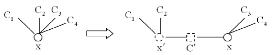
Figure 8: Transform a bit node of degree 4 into two bit nodes of degree 3 and an auxiliary check node.

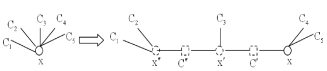
Figure 9: Transform a bit node of degree 5 into three bit nodes of degree 3 and two auxiliary check nodes.

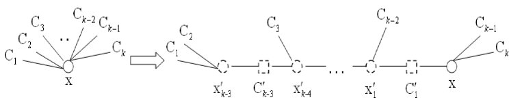
Figure 10: Transform a bit node of degree k into $k-2$ bit nodes of degree 3 and $k-3$ auxiliary check node.

Proof: We first show that an LDPC code with arbitrary column weight distribution and row weight distribution can be equivalently transformed into an LDPC code with maximum column weight three. For example, Figure 8 on the left shows a bit node $x$ of degree 4. It can be split into two bit nodes $x$ and $x^{\prime}$ of degree 3 and an auxiliary check node $C^{\prime}$, as shown on the right in Figure 8. The auxiliary check node $C^{\prime}$ is represented as $x\oplus x^{\prime}=0$, which means $x$ is equivalent to $x^{\prime}$. Originally the bit node $x$ connects to four check nodes $C_{1}$, $C_{2}$, $C_{3}$, and $C_{4}$. After node splitting, $x^{\prime}$ connects to $C_{1}$, $C_{2}$, and $x$ connects to $C_{3}$, $C_{4}$. Hence, the Tanner graph on the left in Figure 8 is equivalent to the Tanner graph on the right in Figure 8. Similarly, a bit node of degree 5 can be split into three bit nodes $x$, $x^{\prime}$, and $x^{\prime\prime}$ and two auxiliary check nodes $C^{\prime}$ and $C^{\prime\prime}$, as shown in Figure 9. Generally, a bit node of degree $k$ can be equivalently transformed into $k-2$ bit nodes of degree 3 and $k-3$ auxiliary check nodes, as shown in Figure 10. Assume an LDPC code $\mathcal{C}$ contains $M$ check nodes and $N$ bit nodes. The $M$ check nodes have degrees $k_{1}$, $k_{2}$, $\ldots$, $k_{M}$, respectively. The $N$ bit nodes have degrees $j_{1}$, $j_{2}$, $\ldots$, $j_{N}$, respectively. Among the $N$ bit nodes in $\mathcal{C}$, there are $s$ bit nodes whose degrees are greater than 3 and their degrees are $j_{1}$, $j_{2}$, $\ldots$, $j_{s}$. This LDPC code can be equivalently transformed into another LDPC code $\mathcal{C^{\prime}}$ with maximum column weight 3. The new code $\mathcal{C^{\prime}}$ has $M+\left(\sum_{i=1}^{s}j_{i}-3s\right)$ check nodes and $N+\left(\sum_{i=1}^{s}j_{i}-3s\right)$ bit nodes. By Theorem 3, the LDPC code $\mathcal{C^{\prime}}$ can be encoded in linear time and the encoding complexity is less than $2\cdot M^{\prime}\cdot(\overline{k^{\prime}}-1)$. where $M^{\prime}$ is the number of independent check nodes in $\mathcal{C^{\prime}}$ and $\overline{k^{\prime}}$ is the average degree of independent check nodes in $\mathcal{C^{\prime}}$. Since there are $\sum_{i=1}^{s}j_{i}-3s$ auxiliary check nodes in $\mathcal{C^{\prime}}$ that have degree 2, we derive that

$$2\cdot M^{\prime}\cdot(\overline{k^{\prime}}-1) = 2\cdot\left(M\cdot(\overline{k}-1)+\left(\sum_{i=1}^{s}j_{i}-3s\right)\cdot(2-1)\right)$$ (13)

$$< 2\cdot\left(M\cdot(\overline{k}-1)+\left(\sum_{i=1}^{N}j_{i}-N\right)\right)$$

$$< 2\cdot\left(M\cdot(\overline{k}-1)+\left(\sum_{i=1}^{M}k_{i}-M\right)\right)$$

$$= 4\cdot M\cdot(\overline{k}-1)$$

Therefore, the overall computation cost of encoding $\mathcal{C}^{\prime}$ is less than $4\cdot M\cdot(\overline{k}-1)$. As the LDPC code $\mathcal{C}$ is equivalent to the LDPC code $\mathcal{C}^{\prime}$, the complexity of encoding $\mathcal{C}$ is less than $4\cdot M\cdot(\overline{k}-1)$. This completes the proof. $\Box$

Let’s look at an example. The parity check matrix of a (13,26) LDPC code with column weight 3 is shown in (14). Assume the values of the 13 information bits are 0, 1, 1, 1, 0, 1, 1, 0, 0, 1, 0, 1, and 1. We apply the proposed linear complexity encoding method to encode this code.

$$\mathbf{H}=\begin{array}[]{c}\left[\begin{array}[]{cccccccccccccccccccccccccc}1&0&0&0&0&0&0&0&1&0&0&0&1&0&0&0&0&0&0&0&1&1&1&0&0&0\\ 0&0&0&1&0&0&0&1&0&0&0&1&0&0&0&1&0&1&0&0&0&0&1&0&0&0\\ 0&0&1&0&0&0&0&0&0&0&1&0&0&0&1&0&0&0&0&1&0&0&0&0&1&1\\ 0&0&0&0&0&0&1&1&0&1&0&0&0&1&0&0&0&0&0&0&1&0&0&1&0&0\\ 0&0&0&0&0&1&0&0&0&0&0&0&0&0&1&0&0&0&1&1&0&0&0&0&1&1\\ 0&0&0&0&1&0&1&0&0&0&0&1&1&0&0&0&1&0&0&0&0&0&1&0&0&0\\ 0&0&0&0&1&0&0&0&1&0&0&0&1&1&0&1&0&1&0&0&0&0&0&0&0&0\\ 0&0&1&0&0&1&0&0&0&0&1&0&0&0&0&0&0&0&1&0&0&0&0&1&1&1\\ 0&1&0&1&0&0&1&0&0&0&0&0&0&0&0&1&0&0&0&0&0&1&0&1&0&0\\ 0&1&0&0&0&0&0&0&1&1&0&1&0&1&0&0&0&1&0&0&0&0&0&0&0&0\\ 0&0&1&0&0&1&0&0&0&0&1&0&0&0&1&0&0&0&1&1&0&0&0&0&0&0\\ 1&1&0&0&0&0&0&1&0&0&0&0&0&0&0&0&1&0&0&0&1&0&0&0&0&0\\ 1&0&0&1&1&0&0&0&0&1&0&0&0&0&0&0&1&0&0&0&0&1&0&0&0&0\end{array}\right]\end{array}$$ (14)

Preprocessing. We construct an encoding stopping set from (14) using Algorithm 5. We start from an empty graph $\mathcal{S}$ and add check nodes and their associated bit nodes to $\mathcal{S}$. Each time we add a check node, we always pick the check node that contains the smallest number of outsider nodes of $\mathcal{S}$. After adding 7 check nodes, the resulting graph is a pseudo-tree, as shown in Figure 11. When 9 check nodes are considered, we get the 2-fold-constraint encoding stopping set $\mathcal{E}_{1}$ shown in Figure 12. The bits $x_{9},\,\,x_{13},\,\,x_{22},\,\,x_{23},\,\,x_{5},\,\,x_{16},\,\,x_{4},\,\,x_{12},\,\,x_{17}$ are information bits. The two check nodes $C_{10}$ and $C_{12}$ are key check nodes, and the two bit nodes $x_{1}$ and $x_{18}$ are reevaluated bits.

After finding the encoding stopping set $\mathcal{E}_{1}$, the remaining Tanner graph of the code can be constructed to be a 2-fold-constraint encoding stopping set $\mathcal{E}_{2}$, as shown in Figure 13. Therefore, the LDPC code can be partitioned into two encoding stopping sets $\mathcal{E}_{1}$ and $\mathcal{E}_{2}$ that are shown in Figure 13. The bits $x_{11},\,\,x_{15},\,\,x_{19},\,\,x_{25}$ in the encoding stopping set $\mathcal{E}_{2}$ are information bits. The two check nodes $C_{3}$ and $C_{5}$ are key check nodes of $\mathcal{E}_{2}$, and the two bit nodes $x_{3}$ and $x_{6}$ are reevaluated bits of $\mathcal{E}_{2}$.

Encoding.

• Fill the values of the information bits, i.e., $[x_{9}\,\,x_{13}\,\,x_{22}\,\,x_{23}\,\,x_{5}\,\,x_{16}\,\,x_{4}\,\,x_{12}\,\,x_{17}]$ = [0    1    1    1    0    1    1    0    0]. Assign $x_{1}=0$ and $x_{18}=0$.

• Encode the pseudo-tree shown in Figure 11. Compute the parity bits $x_{21}$, $x_{14}$, $x_{8}$, $x_{7}$, $x_{10}$, $x_{24}$, $x_{2}$ as follows.

  $$x_{21} = x_{1}\oplus x_{9}\oplus x_{13}\oplus x_{22}\oplus x_{23}=1$$

  $$x_{14} = x_{9}\oplus x_{13}\oplus x_{5}\oplus x_{16}\oplus x_{18}=0$$

  $$x_{8} = x_{23}\oplus x_{16}\oplus x_{18}\oplus x_{4}\oplus x_{12}=1$$

  $$x_{7} = x_{13}\oplus x_{23}\oplus x_{5}\oplus x_{12}\oplus x_{17}=0$$

  $$x_{10} = x_{1}\oplus x_{22}\oplus x_{5}\oplus x_{4}\oplus x_{17}=0$$

  $$x_{24} = x_{21}\oplus x_{14}\oplus x_{8}\oplus x_{7}\oplus x_{10}=0$$

  $$x_{2} = x_{22}\oplus x_{24}\oplus x_{16}\oplus x_{7}\oplus x_{4}=1$$

• Compute the values of the parity check equations $C_{10}$ and $C_{12}$. $\widetilde{C_{10}}=x_{2}\oplus x_{9}\oplus x_{10}\oplus x_{12}\oplus x_{14}\oplus x_{18}=1$, and $\widetilde{C_{12}}=x_{1}\oplus x_{2}\oplus x_{8}\oplus x_{17}\oplus x_{21}=1$.

• Since $\widetilde{C_{10}}=1$ and $\widetilde{C_{12}}=1$, the correct values of $x_{1}$ and $x_{18}$ are $x_{1}=\widetilde{C_{10}}=1$ and $x_{18}=\widetilde{C_{12}}=1$.

• Recompute the parity bits $x_{21}$, $x_{14}$, $x_{8}$, and $x_{10}$ based on the new values of $x_{1}$ and $x_{18}$. We derive that $x_{21}=0$, $x_{14}=1$, $x_{8}=0$, $x_{10}=1$.

• Fill the values of the information bits, i.e., $[x_{11}\,\,x_{15}\,\,x_{19}\,\,x_{25}]$ = [1    0    1    1]. Assign $x_{3}=0$ and $x_{6}=0$.

• Compute the parity bits $x_{20}$, $x_{26}$ as follows.

  $$x_{20} = x_{3}\oplus x_{6}\oplus x_{11}\oplus x_{15}\oplus x_{19}=0$$

  $$x_{26} = x_{3}\oplus x_{6}\oplus x_{11}\oplus x_{19}\oplus x_{25}\oplus x_{24}=1$$

  Notice that the value of the parity bit $x_{26}$ is based on the value of the bit $x_{24}$ in $\mathcal{E}_{1}$.

• Compute the values of the parity check equations $C_{3}$ and $C_{5}$. $\widetilde{C_{3}}=x_{3}\oplus x_{20}\oplus x_{11}\oplus x_{15}\oplus x_{26}\oplus x_{25}=1$, and $\widetilde{C_{5}}=x_{6}\oplus x_{20}\oplus x_{15}\oplus x_{19}\oplus x_{26}\oplus x_{25}=1$.

• Since $\widetilde{C_{3}}=1$ and $\widetilde{C_{5}}=1$, the correct values of $x_{3}$ and $x_{6}$ are $x_{3}=\widetilde{C_{3}}=1$ and $x_{6}=\widetilde{C_{5}}=1$.

The encoded codeword is

$[x_{9}\,\,x_{13}\,\,x_{22}\,\,x_{23}\,\,x_{5}\,\,x_{16}\,\,x_{4}\,\,x_{12}\,\,x_{17}\,\,x_{1}\,\,x_{18}\,\,x_{21}\,\,x_{14}\,\,x_{8}\,\,x_{7}\,\,x_{10}\,\,x_{24}\,\,x_{2}\,\,x_{11}\,\,x_{15}\,\,x_{19}\,\,x_{25}\,\,x_{3}\,\,x_{6}\,\,x_{20}\,\,x_{26}]=[0\,\,1\,\,1\,\,1\,\,0\,\,1\,\,1\,\,0\,\,0\,\,1\,\,1\,\,0\,\,1\,\,0\,\,0\,\,1\,\,0\,\,1\,\,1\,\,0\,\,1\,\,1\,\,1\,\,1\,\,0\,\,1]$

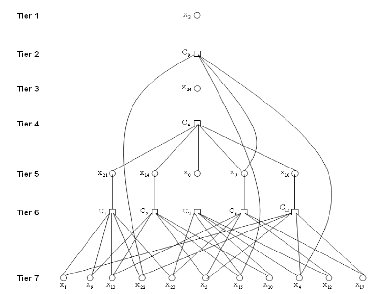
Figure 11: A pseudo-tree built from the LDPC code described in (14).

Figure 12: An encoding stopping set developed from the LDPC code described in (14).

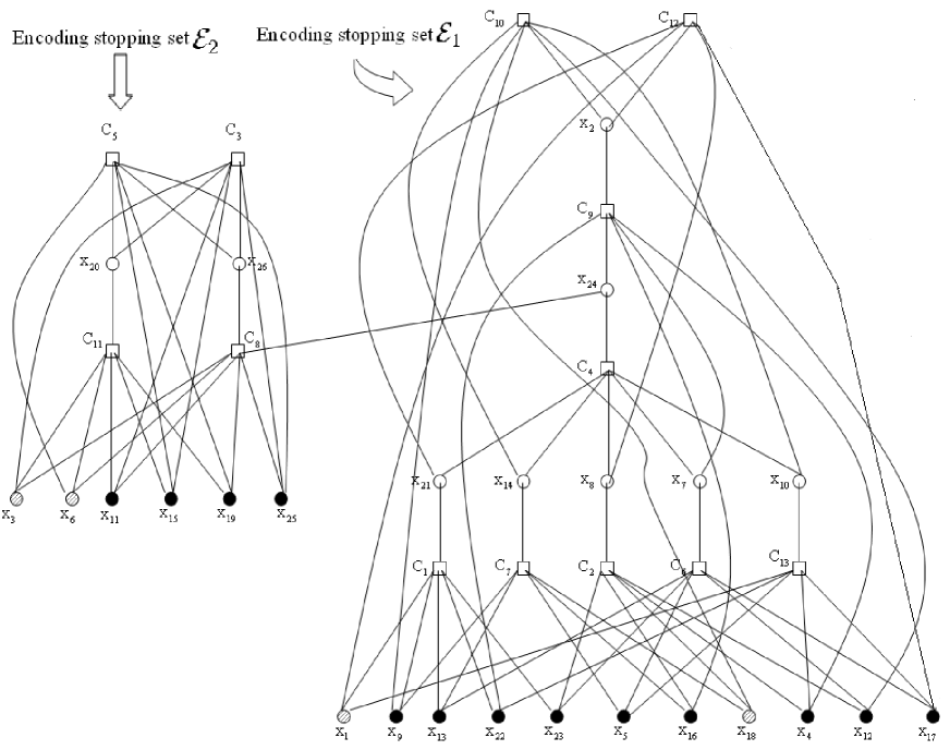
Figure 13: Two encoding stopping sets developed from the LDPC code described in (14).

VIII Conclusion

This paper proposes a linear complexity encoding method for general LDPC codes by analyzing and encoding their Tanner graphs. We show that two particular types of Tanner graphs–pseudo-trees and encoding stopping sets can be encoded in linear time. Then, we prove that any Tanner graph can be decomposed into pseudo-trees and encoding stopping sets. By encoding the pseudo-trees and encoding stopping sets in a sequential order, we achieve linear complexity encoding for arbitrary LDPC codes. The proposed method can be applied to a wide range of codes; it is not limited to LDPC codes. It is applicable to both regular LDPC codes and irregular LDPC codes. It is also good for both “low density” parity check nodes and “medium-to-high density” parity check nodes. In fact, the proposed linear time encoding method is applicable to any type of block codes. It removes the problem of high encoding complexity for all long block codes that historically are commonly encoded by matrix multiplication.

Appendix A
Finding reevaluated bits $x_{\gamma}$ and $x_{\delta}$ in a 2-fold-constraint encoding stopping set

The details are described in Algorithm 8.

Algorithm 8 Finding reevaluated bits $x_{\gamma}$ and $x_{\delta}$ in a 2-fold-constraint encoding stopping set

  Represent the two key check equations $C_{\alpha}$ and $C_{\beta}$ as functions of the information bits only. Assume $C_{\alpha}$ is associated with $q$ information bits $x_{\alpha_{1}}$, $x_{\alpha_{2}}$, $\ldots$, $x_{\alpha_{q}}$ and $C_{\beta}$ is associated with $p$ information bits $x_{\beta_{1}}$, $x_{\beta_{2}}$, $\ldots$, $x_{\beta_{p}}$.

  $Flag\leftarrow 0$.

  for $i$ = 1 to $q$ do

     if $x_{\alpha_{i}}$ is contained in $C_{\alpha}$ but not in $C_{\beta}$ then

        $Flag\leftarrow 1$.

        Choose the reevaluated bit $x_{\gamma}$ to be $x_{\gamma}=x_{\alpha_{i}}$.

        exit the for loop.

     end if

  end for

  if $Flag=1$ then

     Choose the reevaluated bit $x_{\delta}$ to be $x_{\delta}=x_{\beta_{p}}$.

  else

     Choose the reevaluated bit $x_{\gamma}$ to be $x_{\gamma}=x_{\alpha_{q}}$.

     for $i$ = 1 to $p$ do

        if $x_{\beta_{i}}$ is contained in $C_{\beta}$ but not in $C_{\alpha}$ then

           Choose the reevaluated bit $x_{\delta}$ to be $x_{\delta}=x_{\beta_{i}}$.

           exit the for loop.

        end if

     end for

  end if

  Output the two chosen reevaluated bits $x_{\gamma}$ and $x_{\delta}$.

References

• [1] R. G. Gallager, Low-Density Parity Check Codes, MIT Press, Cambridge, MA, 1963.
• [2] D. J. C. Mackay, “Good error-correcting codes based on very sparse matrices,” IEEE Trans. Inform. Theory, vol. 45, no. 2, pp. 399–431, March 1999.
• [3] G. Berrou and A. Glavieux and P. Thitimajshima, “Near Shannon limit error-correcting coding: Turbo codes,” Proc. 1993 International Conf. Comm, pp. 1064-1070, Geneva, Switzerland, May, 1993.
• [4] J. Lu, José M. F. Moura, and H. Zhang, “Efficient encoding of cycle codes: a graphical approach,” Proc. of 37th Asilomar Conference on Signals, Systems, and Computers, pp. 69-73, PACIFIC GROVE, CA, Nov. 9-12, 2003.
• [5] Z. Li, L. Chen, L. Zeng, S. Lin, and W. H. Fong, “Efficient encoding of quasi-cyclic low-density parity-check codes,” IEEE Trans. Comm., vol. 54, no. 1, pp. 71–81 Jan. 2006.
• [6] T. Mittelholzer, “Efficient encoding and minimum distance bounds of Reed-Solomon-type array codes,” Proc. of ISIT 2002, pp. 282, Lausanne, Switzerland, 2002.
• [7] J. Lu and José M. F. Moura, “TS-LDPC codes: Turbo-structured codes with large girth,” IEEE Trans. Inform. Theory, vol. 53, no. 3, pp. 1080–1094, Mar. 2007.
• [8] Y. Kou, S. Lin, and M. P. C. Fossorier, “Low-density parity-check codes based on finite geometries: a rediscovery and new results,” IEEE Trans. Inform. Theory, vol. 47, no. 7, pp. 2711–2736, Nov. 2001.
• [9] S. J. Johnson and S. R. Weller “A Family of irregular LDPC codes with low encoding complexity,” IEEE Comm. Letters, vol. 7, no. 2, pp. 79–81, Feb. 2003.
• [10] S. Freundlich, D. Burshtein, and S. Litsyn, “Approximately lower triangular ensembles of LDPC codes with linear encoding complexity,” IEEE Trans. Inform. Theory, vol. 53, no. 4, pp. 1484–1494, Apr. 2007.
• [11] M. Yang, W. E. Ryan, and Y. Li “Design of efficiently encodable moderate-length high-rate irregular LDPC codes,” IEEE Trans. Comm., vol. 52, no. 4, pp. 564–570, Apr. 2004.
• [12] D. Haley, A. Grant, and J. Buetefuer, “Iterative encoding of low-density parity-check codes,” in Proc. of IEEE Globecom 2002, vol. 2, pp. 1289–1293, Taipei, Taiwan, R.O.C., Nov. 2002.
• [13] D. Haley and A. Grant, “High rate reversible LDPC codes,” Proc. of 5th Australian Communications Theory Workshop, pp. 114 -117, Newcastle, Australia, Feb. 2004.
• [14] T. J. Richardson and R. L. Urbanke, “Efficient encoding of low-density parity-check codes,” IEEE Trans. Inform. Theory, vol. 47, no. 2, pp. 638-656, Feb. 2001.
• [15] R. M. Tanner, “A recursive approach to low complexity codes,” IEEE Trans. Inform. Theory, vol. IT-27, no. 5, pp. 533–547, Sep. 1981.
• [16] C. Di, D. Proietti, E. Telatar, T. Richardson, and R. Urbanke, “Finite-length analysis of low-density parity-check codes on the binary erasure channel,” IEEE Trans. Inform. Theory, vol. 48, no. 6, pp. 1570–1579, June 2002.