Shells, jets, and internal working surfaces in the molecular outflow from IRAS 04166+2706

Abstract

Context. IRAS 04166+2706 in Taurus is one of the most nearby young stellar objects whose molecular outflow contains a highly collimated fast component.

Aims. The high symmetry and pristine appearance of this outflow suggests that its study could offer unique clues on the nature of the still mysterious underlying driving wind.

Methods. We have observed the IRAS 04166+2706 outflow with the IRAM Plateau de Bure interferometer in CO(J=2–1) and SiO(J=2–1) achieving angular resolutions between $2^{\prime\prime}$ and $4^{\prime\prime}$. To improve the quality of the CO(2–1) images, we have added single dish data to the interferometer visibilities.

Results. The outflow consists of two distinct components. At velocities $<10$ km s^-1, the gas forms two opposed, approximately conical shells that have the YSO at their vertex. These shells coincide with the walls of evacuated cavities and seem to result from the acceleration of the ambient gas by a wide-angle wind. At velocities $>30$ km s^-1, the gas forms two opposed jets that travel along the center of the cavities and whose emission is dominated by a symmetric collection of at least 7 pairs of peaks. The velocity field of this component presents a sawtooth pattern with the gas in the tail of each peak moving faster than the gas in the head. This pattern, together with a systematic widening of the peaks with distance to the central source, is consistent with the emission arising from internal working surfaces traveling along the jet and resulting from variations in the velocity field of ejection. We interpret this component as the true protostellar wind, and we find its composition consistent with a chemical model of such type of wind.

Conclusions. Our results support outflow wind models that have simultaneously wide-angle and narrow components, and suggest that the EHV peaks seen in a number of outflows consist of internally-shocked wind material.

1 Introduction

Bipolar outflows powered by young stellar objects (YSOs) still pose a number of puzzles almost three decades after their discovery (Snell et al. 1980). Although it is now well accepted that most of the moving gas seen in an outflow consists of molecular ambient material accelerated by a primary wind, inferring the properties of this wind from observations of the accelerated gas has proven a difficult task (e.g., Bachiller 1996). Part of this difficulty results from the large variety of observed shapes and velocity patterns seen in the outflow accelerated gas, that range from the almost parabolic shells of low velocity material seen in L1551 and Mon R2 (Moriarty-Schieven et al. 1987; Meyers-Rice & Lada 1991) to the collimated jets of fast gas observed towards L1448-mm and HH211 (Bachiller et al. 1990; Gueth & Guilloteau 1999). In addition to the molecular data, optical observations of outflows often reveal an atomic component of higher excitation and collimation, probably resulting from recently shocked material either in the wind itself or at the interface between the wind and the cloud. This atomic component is clearly related to the molecular gas, as the two coincide in sense and direction when both are seen, but the exact connection between these components still remains unclear (Pety et al. 2006). The presence of this component reveals that the outflow phenomenon is both long lived and highly time variable (see Reipurth & Bally 2001 for a review).

A number of wind geometries and kinematics have been proposed over the years to explain outflow observations, and most of the models can be classified as either wide-angle components (e.g., Shu et al. 1991) or highly collimated jets (e.g., Masson & Chernin 1993). Each of these simple geometries has proven successful explaining a subset of the observed outflows: wide-angle winds can easily explain shell outflows, while jets have been used to model highly collimated flows. None of these models, however, seems capable of explaining simultaneously all types of outflows (Lee et al. 2002), and this suggests that each of them only provides a partial description of the outflow phenomenon.

In recent years, a new generation of outflow models with both collimated and wide-angle wind components has been presented (Banerjee & Pudritz 2006; Shang et al. 2006; Machida et al. 2008). At the same time, a significant increase in the sensitivity and resolution of millimeter and submillimeter interferometers such as the PdBI, SMA, or CARMA has started to allow mapping the relatively weak emission from outflows with a detail approaching that of the optical and IR observations of Herbig-Haro objects and jets. This combination of theoretical and observational advances has opened the possibility of carrying out a new generation of outflow studies that may finally reach a consistent picture of outflows. Such a picture should not only describe the variety of observed morphologies and kinematics, but bring together, in a single evolutionary sequence, both the molecular outflows from the most embedded objects and the optical jets of some TTauri stars.

Previous studies of low-mass outflows have shown that those from the youngest stellar objects display the simplest geometry and kinematics, probably due to their limited distortion by anisotropies in the surrounding environment (Arce et al. 2007). These youngest outflows often present in the spectra a distinct secondary component at velocities over 30 km s^-1, which is often referred to as the extremely high velocity (EHV) gas (Bachiller 1996). Because of their pristine appearance, these young outflows are ideal targets to attempt inferring properties of the invisible wind from the observation of the accelerated gas. Among the youngest protostars known, IRAS 04166+2706 (I04166 hereafter) stands out for its close location (Taurus molecular cloud, at 140 pc), simple environment (the B213 filament), and high symmetry of its bipolar outflow. The flow from this 0.4 L_⊙ object was first reported by Bontemps et al. (1996), who mapped its low velocity gas towards the vicinity of the YSO. Further observations with the IRAM 30m telescope by Tafalla et al. (2004) (TSJB04 hereafter) revealed a spectacular outflow extending over at least $400^{\prime\prime}$ ($>0.25$ pc) and presenting a component of EHV gas that contains half of the outflow total momentum and 80% of its kinetic energy, and so collimated that could not be resolved with a beam of $\approx 11^{\prime\prime}$ FWHM. In this paper, we present new high resolution interferometric observations of the central $\approx 0.1$ pc of the outflow. These new data allow us to separate the distributions of the EHV gas and the lower velocity component, and their analysis provides new clues on the nature of the outflow driving wind.

2 Observations

We observed the inner part ($\sim 200^{\prime\prime}\times 40^{\prime\prime}$) of the I04166 bipolar outflow using the IRAM Plateau de Bure Interferometer (PdBI) in its CD configuration during the winters of 2004-05 (blue lobe) and 2005-06 (red lobe). The receivers were tuned simultaneously to SiO(J=2–1) (86.8 GHz) and CO(J=2–1) (230.5 GHz), and the correlator was configured to provide velocity resolutions of 1.6 and 1.1 km s^-1 for the two transitions, respectively. A broad band mode of the correlator was also used to provide 1 GHz of bandwidth at each frequency for making maps of the continuum emission. In order to cover the extended emission of the outflow, each lobe was observed with a mosaic of 18 fields, and the central two fields around I04166 were observed in the two epochs to check and ensure the consistency of the calibration (found to be better than 10% for the continuum at both 1 and 3 mm).

The observations of I04166 were interspersed with observations of nearby quasars to track possible variations of the instrumental gains during the observation. These calibrator observations were used to correct the I04166 data, and the calibrated visibilities were inverted and CLEANed to generate maps using the GILDAS software. Comparing the resulting interferometer spectra with single dish observations from the IRAM 30m telescope, we estimate that the interferometer observations recover close to 100% of the flux from the SiO(2–1) emission. For CO(2–1), the interferometer data recover about 40% of the flux at the highest velocities and close to 20% at the lowest speeds. To correct for this flux loss, we used the CO(2–1) data presented in TSJB04. From these data, we generated a set of short-spacing visibilities that were added to the PdBI visibilities, and a new series of maps was made. Before merging the data, we found that it was necessary to offset the single dish map by ($4^{\prime\prime}$, -$3^{\prime\prime}$) in order to align the two data sets. Natural or robust weighting provided the best compromise between resolution and sensitivity, and they were used accordingly to generate the final maps. The FWHM of the synthesized beam is about $4^{\prime\prime}\times 3^{\prime\prime}$ for SiO(2–1) and the 3.5 mm continuum and $2^{\prime\prime}\times 2^{\prime\prime}$ for CO(2–1) and the 1.3 mm continuum.

3 Continuum data

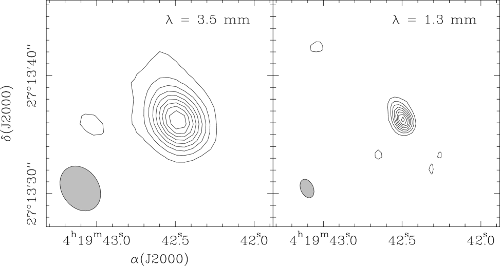
Figure 1: Continuum maps of the vicinity of IRAS 04166+2706 for wavelengths 3.5 mm (left) and 1.3 mm (right). Only the central part of the map is shown because no additional mm sources were detected in the region (see Fig. 3 for the full extent of the map). First contour and contour interval is 1 mJy beam^-1 for 3.5 mm and 7.5 mJy beam^-1 for 1.3 mm. The FWHM of the synthesized beam, indicated with a grey ellipse in each panel, is $4\aas@@fstack{\prime\prime}1\times 3\aas@@fstack{\prime\prime}1$ at 3.5 mm and $1\aas@@fstack{\prime\prime}7\times 1\aas@@fstack{\prime\prime}1$ at 1.3 mm.

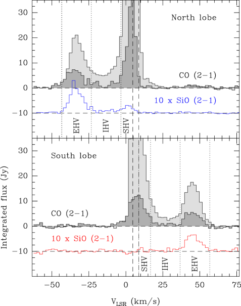
Figure 2: CO(2–1) and SiO(2–1) spectra integrated over the north (blue) and south (red) lobes of the I04166 outflow illustrating the distinct appearance of the EHV, IHV, and SHV regimes (see text). Note how the EHV gas forms well-defined secondary maxima shifted by about 40 km s^-1 to the blue and red of the ambient component (centered at $V_{\mathrm{L}SR}=6.7$ km s^-1). The brighter CO(2–1) spectra in the plot result from combining interferometer and single-dish data, while the weaker counterparts correspond to interferometer-only data. The SiO(2–1) spectra have been scaled and shifted downwards for clarity.

Figure 1 shows maps of the 3.5 and 1.3 mm continuum emission towards the vicinity of I04166. In both panels, the emission presents a well-defined single peak near the nominal IRAS position, and no other mm peak is detected in the mapped region. We interpret this mm peak as the counterpart of the IRAS source, and we determine its location by fitting the visibilities at both wavelengths. The results of these fits, which agree better than one arcsec, indicate that the source is located at $\alpha(J2000)=4^{h}19^{m}42\aas@@fstack{s}5,$ $\delta(J2000)=+27^{\circ}13^{\prime}36^{\prime\prime}$.

The analysis of the interferometer visibilities also shows that the mm emission from the central peak is not resolved by the observations. This means that the region responsible for this emission must be smaller than our beam, which for the 1.3 mm observations is of $1\aas@@fstack{\prime\prime}4$, or about 200 AU at the distance of Taurus. Given this small size, the dust is most likely located in a disk around the protostar, although a contribution from the inner protostellar envelope cannot be totally ruled out (Jørgensen et al. 2007; Chiang et al. 2008). For disk emission in Taurus, it is possible to obtain a reasonably accurate estimate of the disk mass by assuming that the emitting dust is approximately isothermal at a temperature of 20 K (Andrews & Williams 2007). According to the disk model of D’Alessio et al. (1998), this temperature is reached in the disk mid plane within the inner 50 AU from the central object, so the 20 K radius lies well inside our interferometer beam. Assuming a 20 K temperature and a 1.3 mm dust emissivity of 0.01 cm² g^-1 (Ossenkopf & Henning 1994), our measured 1.3 mm flux of $59\pm 2$ mJy implies a disk (gas + dust) mass of approximately 0.02 M_⊙.

Information on the dust physical properties can be derived from the frequency dependence of the dust emissivity. Assuming optically thin emission from 20 K dust and using the above 1.3 mm flux together with the measured 3.5 mm flux of $11\pm 0.5$ mJy, our observations imply a power-law index for the dust emissivity of $\beta=-0.1\pm 0.1$ ($\kappa_{\nu}\sim\nu^{\beta}$). Such a value of $\beta$ is much lower than the canonical ISM value of 2 (Draine & Lee 1984), but it is similar to the values found in other YSOs in Taurus, and it can be understood as resulting from grain growth at the high densities expected in the disk interior (Beckwith & Sargent 1991).

4 Overall outflow morphology

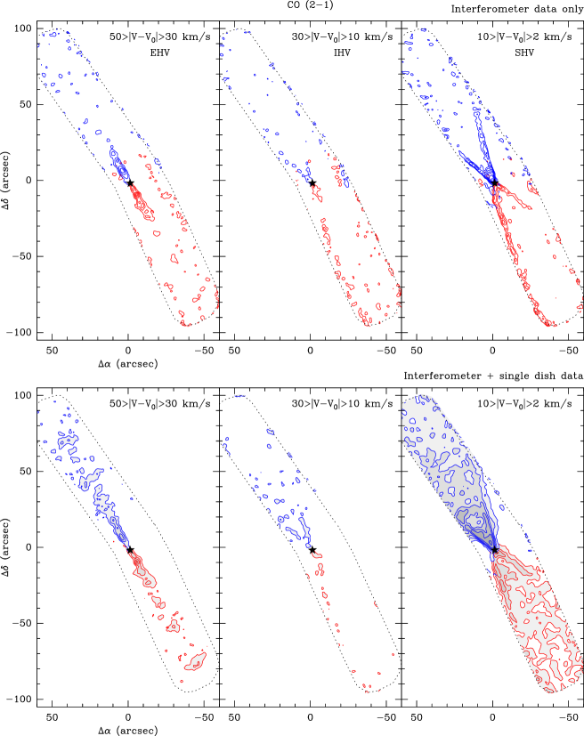
Figure 3: Maps of the CO(2–1) emission towards I04166 integrated over three velocity ranges referred to, by decreasing velocity, as extremely high velocity (EHV), intermediate high velocity (IHV), and standard high velocity (SHV). The top panels show maps made using interferometer data only, which enhances the small-scale structure of the emission. The bottom panels show maps made combining the interferometer data with visibilities derived from single dish (IRAM 30m) observations, and are more sensitive to the low-level, extended emission. Note how the EHV emission consists of a symmetric collection of highly aligned discrete peaks, while the SHV emission forms two shells that surround the EHV jet. The offsets are referred to the phase center of the interferometer observations ($\alpha_{J2000}=4^{\rm h}19^{\rm m}42\aas@@fstack{s}6$, $\delta_{J2000}=27\degr 13^{\prime}38^{\prime\prime}$), the star symbol indicates the location of the mm continuum peak, and V₀ ($=6.7$ km s^-1) corresponds to the velocity of the ambient core as determined from NH₃ observations. In the interferometer-only maps, the first contour and interval are at 6 K km s^-1 for the EHV and IHV ranges and 5 K km s^-1 for SHV. In the combined maps, the first contour and interval are 5 K km s^-1 for all the velocity ranges in the red-shifted gas, and 6 K km s^-1 (EHV and IHV) and 7 K km s^-1 (SHV) in the blue-shifted gas. The dotted line indicates the region covered by the interferometer observations. Beam sizes are approximately $2\aas@@fstack{\prime\prime}5\times 2^{\prime\prime}$ in the interferometer-only maps and $3^{\prime\prime}\times 3^{\prime\prime}$ in the combined maps.

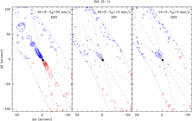
Figure 4: Maps of the SiO(2–1) emission towards I04166 integrated over the same velocity ranges as in Fig. 3. The long-dashed lines that converge into the star symbol (mm peak position) represent the directions of the jet and shells seen in the CO(2–1) map of Fig. 3, and are presented to aid the eye when comparing the emission from the two species. Note how the EHV SiO(2–1) emission presents a similar distribution to the CO(2–1) EHV emission. The IHV and SHV SiO(2–1) emission is only detected toward the northern blue lobe and seems associated to the CO shells. First contour and interval are 2 K km s^-1 and 1.5 K km s^-1 for the EHV and IHV ranges of the blue and red emission, respectively, and 1.5 K km s^-1 and 1 K km s^-1 for the SHV range of the blue and red emission, respectively. Offsets, star symbol, and dotted lines as in Fig. 3 Only interferometer data were used to generate the maps, and the synthesized beam FWHM is approximately $4^{\prime\prime}\times 3^{\prime\prime}$.

To study the properties of the I04166 outflow, we now turn to our interferometer observations of the CO(2–1) and SiO(2–1) emission. From single dish data, TSJB04 found that the CO(2–1) outflow emission presents three distinct velocity regimes referred to as extremely high velocity (EHV), intermediate high velocity (IHV), and standard high velocity (SHV), and which correspond to velocity displacements from the ambient cloud of 50 to 30 km s^-1 (EHV), 30 to 10 km s^-1 (IHV), and 10 to 2 km s^-1 (SHV). This division of the emission in three velocity regimes is also apparent in our high resolution data, and is illustrated in Fig. 2 using the CO(2–1) and SiO(2–1) spectra integrated over each outflow lobe (for CO, both interferometer-only and combined single-dish and interferometer data are presented). As Fig. 2 shows, the EHV regime appears in the spectra as a pair of secondary peaks symmetrically shifted about 40 km s^-1 to the red and blue of the ambient cloud (at $V_{\mathrm{L}SR}=6.7$ km s^-1, see TSJB04), while the SHV regime appears as the characteristic high velocity red and blue wings of an outflow. The IHV regime is characterized as the transition between the two other regimes, and its intensity is significantly weaker than that of the EHV and SHV gas. As the figure also shows, the three regimes are well detected in CO(2–1), while most of the SiO(2–1) emission belongs to the EHV regime.

The spatial location of the three outflow velocity regimes in CO(2–1) is presented in Fig. 3 with two sets of maps. The top set shows interferometer data only, so the maps tend to magnify the highest spatial frequencies and therefore stress the most compact structures. The bottom set of maps was made adding single dish data to the interferometer visibilities and therefore contains the more diffuse emission. As can be seen, both sets of maps reveal the same general behavior: (i) the emission is bipolar with respect to the millimeter source, (ii) it presents a very high degree of collimation at the highest velocities (EHV, leftmost panels), and (iii) appears cometary in the lowest velocity range (SHV, rightmost panels). The main differences between the two sets of maps are the additional emission seen at large distances from the protostar in the combined EHV map and the diffuse component filling the outflow lobes that appears in the combined SHV map. In both sets of maps, the emission at intermediate velocities (IHV, middle panels) is significantly weaker than in the other two velocities and is qualitatively similar to the emission of the slowest gas.

The most remarkable feature of the maps in Fig. 3 is the very different spatial distribution of the EHV and SHV regimes. The high collimation of the EHV emission, especially close to the millimeter source, where it remains unresolved by our $\approx 2\aas@@fstack{\prime\prime}5$ (350 AU) beam, indicates that the fastest gas in the outflow must be located in a jet-like component that travels along a straight line through the center of each lobe. The cometary shape of the SHV emission, on the other hand, suggest that the lowest velocity gas in the outflow moves along two almost-conical shells that surround symmetrically the high velocity jets and have the IRAS source at their vertex. This very different geometry of the extreme velocity regimes suggests that each outflow lobe consists of two distinct physical components, a jet and a shell, and that there is little or no connection between the two. The data, in particular, seem inconsistent with an outflow distribution where all the gas is located in two shells, and where the difference between the jet and the shell arises only from projection, with the shell being the part of the flow moving orthogonal to the line of sight and the jet being the most blue or red shifted part of the same conical flow (see Tafalla et al. 1997 for an application of such a model to the Mon R2 outflow). Such a geometrical interpretation of the emission would require that there is a series of maps at intermediate velocities where the intensity is similar and the outflow shells converge continuously toward the center of the lobes. As seen in the integrated maps of Fig. 3 such a trend is not found, and as seen in the spectra of Fig. 2, the intermediate velocity regime is much weaker than the EHV emission, which clearly is not a continuation of the outflow wing. The shell-only model, in addition, predicts that two jet features should be seen per lobe, one arising from the front and the other from the back of the shell, and that the velocities of these two jet features should be symmetric with respect to the shell regime. Given that in I04166 the difference in velocity between the jet and the shell is larger than 30 km s^-1, and that the shell is moving about 10 km s^-1 with respect to the ambient gas, the shell-only model predicts that each outflow lobe should have a blue and a red jet, which is clearly not the case. We therefore conclude that the shells and jets in I04166 are not the result from a projection effect, but that they represent two separate components of the bipolar outflow. In the next three sections we discuss with more detail the nature and characteristics of these two components, together with some implications for the underlying physics of the driving wind. In the remainder of this section we continue with a description of the overall properties of the outflow.

A complementary view of the I04166 outflow comes from the SiO(2–1) emission, which was observed simultaneously with CO(2–1) and has a factor-of-two lower resolution. The maps of this emission, integrated in the same velocity ranges used for CO, are presented in Fig. 4. These interferometer-only data recover most of the flux, and therefore reflect the true distribution of SiO emission in the region. As Fig. 4 shows, the SiO(2–1) emission in the EHV range has a jet-like distribution very similar to that seen in CO(2–1), especially when taking into account the lower angular resolution of the SiO data. As we will show in section 6, the CO and SiO emissions in this velocity range agree with each other both in spatial distribution and kinematic structure, indicating that they originate from the same jet-like component of the outflow. The intermediate and low velocity ranges (center and right panels in Fig. 4) show much weaker SiO(2–1). The emission is only detected towards the northern blue lobe, and it has a distribution that resembles the CO blue shell. This asymmetry in the SiO emission is real, and it is probably related to the strong (factor of 3) asymmetry found in the intensity of the CO emission for the same velocity range (TSJB04).

5 The shells

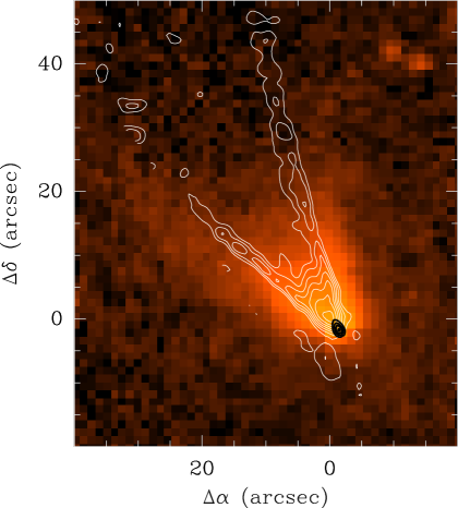
Figure 5: Superposition of the CO(2–1) SHV interferometer-only map (white contours) and the archival $3.6\leavevmode\nobreak\ \mu$m Spitzer IRAC image of I04166 (red scale) illustrating the coincidence of the outflow blue shell and the NIR scattering nebula. The black contours indicate the 1.3 mm continuum emission from the central protostar. Offsets origin and CO contours as in Fig. 3.

As discussed in the previous section, the distribution of CO(2–1) emission in the SHV range suggests that the slowest molecular outflow is confined to the walls of two opposed conical shells. Such a distribution has been seen in other outflows by a number of authors (e.g., Moriarty-Schieven et al. 1987; Meyers-Rice & Lada 1991; Bachiller et al. 1995; Arce & Sargent 2006; Jørgensen et al. 2007) and is naturally explained if the shells represent the walls of two cavities that have been evacuated by the outflow. In the case of I04166, such an interpretation is strengthened by the recent (publicly-available) NIR images of the region taken with the Spitzer Space Observatory’s IRAC camera as part of GO program 3584 (PI: D. Padgett), which show a cometary scattering nebula extending north of the mm source. As illustrated in Fig. 5, this NIR nebula matches nicely the blue CO emission in both direction, shape, and size, as it is expected if the outflow lobe has evacuated the cavity responsible for the nebula. Detailed modeling of the NIR emission shows that the Spitzer images can be reproduced with a scattering nebula that has the geometry suggested by CO if this emission delineates the boundary of the cavity (A. Crapsi, private communication). Furthermore, the opening angle we measure from the CO data ($\approx 32^{\circ}$) is in perfect agreement with the angle determined independently by Seale & Looney (2008) from the NIR Spitzer images (note how in Fig. 5 the NIR emission penetrates slightly the walls of the CO cavity, as expected from the scattering model, but it does so in a way that preserves the opening angle). Finally, we note that the recent N₂H⁺(1–0) OVRO map from Chen et al. (2007) reveals an hourglass distribution of the dense gas that has its waist perpendicular to the outflow axis. This is the geometry expected if the outflow had carved a pair of opposed cavities in the dense core that surrounds the protostar.

We can use the CO and NIR data to constrain the orientation of the outflow axis with respect to the line of sight assuming the shells are conical. Both the absence of direct light from the central protostar in the optical/NIR images and the lack of overlap between the north and south CO lobes imply that the angle between the outflow direction and the line of sight is larger than half the cavity opening angle, or $\approx 16^{\circ}$. On the other hand, the lack of a scattering nebula towards the southern red lobe and the lack of mixing between blue and red gas in each of the outflow lobes (assuming the gas moves along the shells, see below) imply that the orientation angle should be smaller than 74 (=90-16) degrees (Cabrit & Bertout 1990). Although any inclination between the above two extreme limits could be a priori consistent with the observations, the true value is likely to be rather intermediate. A detailed modelling of the NIR scattering nebula (A. Crapsi, private communication) suggests an inclination of 45 degrees, and in the following, we will use this angle as a reference for any kinematics estimate.

An inspection of the individual channel maps in the low velocity regime shows that the opening angle of the CO shells does not change with velocity over the whole SHV range. This behavior suggests that the outflow motions we observe are mostly directed along the shells, and that any perpendicular component of the velocity field is likely to be negligible (see Meyers-Rice & Lada 1991 for a detailed analysis of a similar case in Mon R2). The CO shells, in addition, can be seen in velocity maps that span a range of at least 10 km s^-1, so the material in the SHV regime must span a similar range of longitudinal velocities. This coexistence of material moving along the shells with a large range of velocities can be understood if the low velocity outflow consists of a shear flow of accelerated ambient gas moving along the walls of the evacuated cavities. To produce such a velocity pattern, the driving wind of the outflow must have a speed of at least 10 km s^-1 with respect to the ambient cloud. Although the EHV gas satisfies this requirement and has enough momentum (TSJB04), it is unlikely to constitute the accelerating agent of the SHV gas. As we will see in the next section, the EHV component shows no evidence for momentum transfer to the ambient gas and its opening angle is smaller than the $>30^{\circ}$ opening angle measured in the SHV shells. The SHV gas, therefore, is most likely accelerated by a different (and invisible) component that emerges from the central YSO with a velocity of at least 10 km s^-1 and an opening angle of at least $30^{\circ}$. The straight cavity walls and the highly directed velocity field of the CO SHV suggests that this component has certain degree of collimation, although a more detailed analysis of the interaction between the outflow and the dense gas is needed to reach a firm conclusion. On-going PdBI observations of the core material around I04166 will hopefully shed new light on this important issue.

6 The jets

6.1 Integrated emission

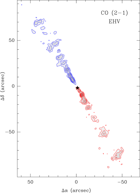
Figure 6: Clipped CO(2–1) map of the EHV regime showing an enhanced view of the fastest part in the I04166 outflow. The map has been made using single dish and interferometer visibilities, and before adding the individual channels, the emission has been clipped at 0.5 K (blue) and 0.3 K (red). First contour and interval are 3.5 K km s^-1 (blue) and 2.5 K km s^-1 (red). Offsets and star symbol are as in Fig. 3.

The maps of integrated intensity for the EHV range shown in Fig. 3 do not provide the best view of the highest velocity component in the outflow, as the 20 km s^-1-wide velocity integral dilutes significantly the emission and makes some low-level features disappear in the noise of the emission-free channels. Due to the internal velocity structure of the EHV gas (see next section), maps with a narrower velocity range do not provide a complete view of this component either, so to achieve the best representation of the EHV gas we resort to maps where the low-level emission has been clipped before integrating in velocity. Figure 6 presents the clipped version of the combined interferometer plus single dish CO(2–1) emission map and shows a better defined structure than the equivalent non clipped version of Figure 3. As the clipped map illustrates, the EHV gas, in addition of being highly collimated, is very fragmented, and it seems to consist more of a collection of discrete emission peaks than a smooth and continuous jet.

Table 1: Properties of EHV peaks from 2D gaussian fits.

$$\begin{array}[]{ccccc}\hline\cr\vskip 3.0pt plus 1.0pt minus 1.0pt\cr\mbox{Name}&\mbox{Position${}^{(1)}$}&\mbox{I[CO(2--1)]${}^{(2)}$}&\mbox{I[SiO(2--1)]${}^{(2)}$}&\mbox{M${}^{(3)}$}\\ &(^{\prime\prime},^{\prime\prime})&\mbox{(K km s${}^{-1})$}&\mbox{(K km s${}^{-1})$}&\mbox{($10^{-5}$ M${}_{\odot}$)}\\ \vskip 3.0pt plus 1.0pt minus 1.0pt\cr\hline\cr\vskip 3.0pt plus 1.0pt minus 1.0pt\cr\mbox{R1}&(-2.3,-3.2)&11.7&7.2&2.2\\ \mbox{R2}&(-5.0,-7.6)&20.4&11.9&4.2\\ \mbox{R3}&(-7.5,-14.1)&12.9&6.9&5.1\\ \mbox{R4}&(-11.9,-21.3)&9.6&2.4&2.4\\ \mbox{R5}&(-18.4,-33.1)&4.8&1.5&3.4\\ \mbox{R6}&(-28.8,-48.9)&7.5&2.0&5.9\\ \mbox{R7}&(-43.8,-73.0)&8.1&1.3&7.4\\ \mbox{B2}&(6.0,9.7)&19.2&18.9&5.9\\ \mbox{B3}&(8.3,13.8)&17.1&20.3&2.3\\ \mbox{B4}&(11.2,19.8)&15.3&13.1&3.1\\ \mbox{B5}&(18.8,33.1)&10.2&9.0&6.0\\ \mbox{B6}&(26.5,46.5)&9.0&2.0&8.8\\ \mbox{B7}&(42.2,71.5)&7.2&5.4&8.0\\ \hline\cr\end{array}$$

• (1) Offsets with respect to the mm-continuum peak at $\alpha(J2000)=4^{h}19^{m}42\aas@@fstack{s}5,$ $\delta(J2000)=+27^{\circ}13^{\prime}36^{\prime\prime}$; (2) peak intensity from 2D gaussian fit; (3) see text for assumptions.

To study the properties of the EHV peaks, we have fitted their CO(2–1) emission in the clipped map with 2D gaussians using the GAUSS_2D routine of the GILDAS program GreG. The results of this fitting are summarized in Table 1 and presented graphically in the left panel of Fig.7 superposed to the EHV emission. With these fits, we can quantify some of the properties of the peaks, and in particular, study the symmetry of their distribution. This is presented graphically in the right panel of Fig. 7, where we have plotted the profiles of the gaussian fits as a function of distance to the mm source. As can be seen, except for peak 1, which seems missing in the blue lobe (a possible result of the clipping), all the other 6 peaks appear both in the red and blue outflow lobes with an almost perfect one-to-one correspondence. In fact, the mean difference between the distance of the blue and red peaks to the central source is less than $2^{\prime\prime}$, which is comparable to the beam size of the observations. Such a regular distribution of the peaks with respect to the central source makes I04166 one of the most symmetric outflows known.

The 2D fits to the CO emission provide additional information on the EHV component. A least squares fit to the peak positions (dashed line in the left panel of Fig. 7) indicates that that the outflow lies at PA = $30\aas@@fstack{\circ}4$ (east or north) with a dispersion of $0\aas@@fstack{\circ}2$. Such a low angular dispersion confirms the almost perfect alignment between the CO peaks, and suggests that any precession or bending of the jet-like component of the outflow must be significantly smaller than one degree.

While the peak alignment is better than one degree, the opening angle of the EHV jet is larger. As can be seen even in the non clipped images, the EHV peaks broaden with distance from the mm source, especially in the direction perpendicular to the jet. This broadening of the peaks is accompanied in some cases (like B6, B7, and R7) by a slight curvature of the emission, which gives the peaks the appearance of bow-shocks propagating away from the source. Using the results from the 2D fits to the 3 outermost peaks of each lobe (numbers 5 to 7) we derive from a least squares fit an opening angle of 10 degrees for the EHV gas. This angle is 3 times smaller than the opening angle of the shells, suggesting again that the jet and the shells are independent outflow components. In particular, it seems unlikely that in the region we have observed, the shells have been accelerated by the precession or broadening of the jet.

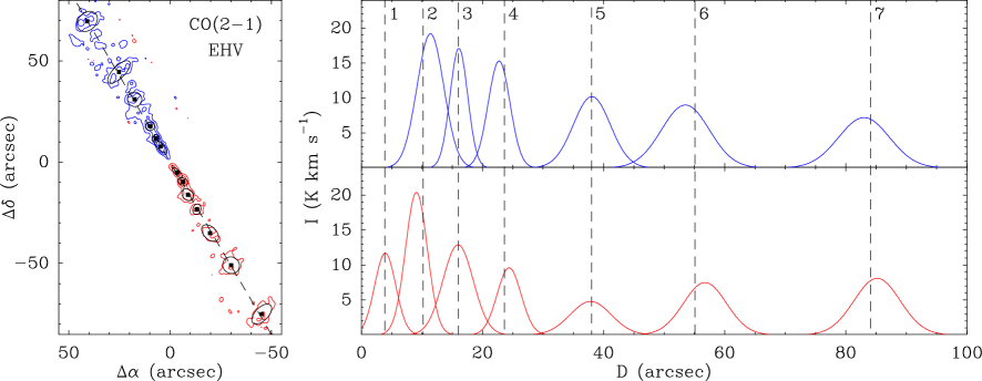
Figure 7: Left:  EHV CO(2–1) clipped emission map as in Fig. 6 (blue and red contours) with the results from 2D gaussian fits to the emission peaks (in black). The solid squares represent the centers of the gaussians and the ellipses represent the fit half maximum contours. The dashed line traces the result from a least squares fit to the gaussian centers and has a dispersion of less than one degree (see text). Right:  2D gaussian fit results as a function of distance to the mm peak (blue lobe in top panel and red lobe in bottom panel). For each EHV peak, the plot shows a gaussian having the fit intensity, distance to the mm peak, and a width given by the geometric mean of the widths from the 2D fit. Note the blue/red symmetry in the position of the peaks, and the decrease in intensity and widening of the gaussians with distance to the source.

In addition to broadening, the peak CO emission from the EHV features weakens with distance to the mm source, as can be seen in the right panel of Fig. 7. This effect, which is again symmetric in the two lobes, is more than compensated by the broadening of the features, so the outermost EHV peaks have a slightly (factor of 2) larger integrated intensity than the innermost peaks. We can use this CO(2–1) integrated intensity to estimate the mass of each peak. The detection of SiO(2–1) guarantees a relatively high density (section 6.3), so LTE conditions are likely to apply to the CO-emitting gas. A more complex issue concerns the temperature and CO abundance of this gas. In TSJB04, we assumed a $T_{\mathrm{e}x}$ of 20 K and a standard Taurus CO abundance of $8.5\;10^{-5}$ (Frerking et al. 1982). As discussed below, however, the kinetic temperature of the EHV gas is likely to be significantly higher than 20 K, and the CO abundance is also expected to exceed $8.5\;10^{-5}$ if this gas represents a protostellar wind instead of accelerated ambient material. Fortunately, the mass determination depends on a ratio where the two effects almost cancel each other, so if, for example, the excitation temperature is as high as 500 K (section 6.3) and the CO abundance is as high as $4\;10^{-4}$ (predicted by the protostellar wind models from Glassgold et al. 1991 and discussed also in section 6.3), the mass estimate is only a factor of 2 higher than predicted using the assumptions in TSJB04. Thus, and for consistency with the interpretation in section 6.3, we use the higher temperature and higher abundance assumptions, although the effect of this choice is relatively small given all the uncertainties in the estimate. Using these values, we have estimated the masses given in Table 1, which indicate that the typical mass of an EHV peak is $5\;10^{-5}$ M_⊙ and the total mass in this outflow component is about $6.5\;10^{-4}$ M_⊙. Dividing this mass by the kinematical age of the outermost peak (1,400 yr, assuming a velocity of 40 km s^-1), we derive a mean mass loss for the EHV gas of about $5\;10^{-7}$ M_⊙ yr^-1.

The combination of (i) symmetry in the location of the peaks with respect to the mm source, (ii) high collimation, and (iii) systematic broadening with distance makes the EHV molecular emission of I04166 very similar to the optical emission of some highly collimated Herbig Haro jets like HH34 and HH111 (Reipurth & Bally 2001). Molecular outflows from other Class 0 sources like L1448-mm (Bachiller et al. 1990), HH211 (Gueth & Guilloteau 1999), and HH212 (Codella et al. 2007; Cabrit et al. 2007; Lee et al. 2008), among others, show similar (although less extreme) behavior, indicating that the properties of I04166 are not peculiar to this source but reflect properties of a wide class of bipolar outflows. The symmetry in the location of the peaks at each side of the central source, in particular, suggests that the production of the EHV peaks is related to some type of episodic event in the outflow source, which based on the kinematic ages of the peaks, has a time scale of the order of 100 years. In addition, the high collimation of the emission indicates that the source is able to produce a jet-like component simultaneously with the wider wind responsible for the shells. To further constrain the origin of the EHV gas, we need to study its kinematic properties.

6.2 Kinematics

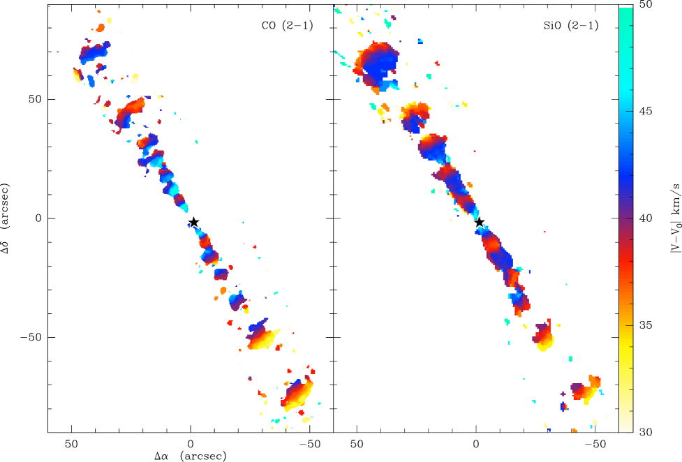
Figure 8: CO(2–1) (left) and SiO(2–1) (right) first momentum maps showing the difference between the velocity of the EHV outflow gas and the ambient cloud in absolute value. Note the oscillating velocity pattern To enhance the S/N, the emission has been clipped before making the EHV maps. Offset center and star symbol are as in Fig. 3.

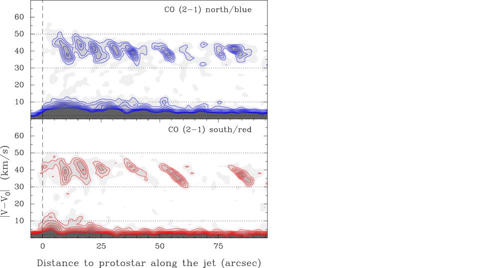
Figure 9: Position-velocity diagrams of the CO(2–1) emission along the outflow axis (blue gas in top panel and red gas in bottom panel). For each lobe, the absolute value of the difference between the outflow and the ambient cloud velocities is presented. Note the discrete EHV peaks in the $30<|V-V_{0}|<50$ km s^-1 interval (enclosed by dotted lines). Each of these peaks presents an internal velocity gradient with the gas closer to the protostar moving faster than the gas at further distances. Despite these gradients, the mean speed of the EHV gas remains constant at about 40 km s^-1, and the overall velocity profile has a characteristic sawtooth pattern. First contour and interval are 0.4 K and 0.2 K respectively, and $V_{0}=6.7$ km s^-1. To enhance the signal-to-noise ratio, the emission has been convolved by $5^{\prime\prime}$ perpendicular to the direction of the cut. No clipping has been applied to these data.

In addition to high collimation and symmetry, the EHV peaks in I04166 present a systematic pattern of internal velocity gradients. Figure 8 illustrates this pattern with the first moment of absolute velocity measured with respect to the ambient cloud ($V_{\mathrm{L}SR}=6.7$ km s^-1, see TSJB04). As it can be seen, both in CO(2–1) and SiO(2–1) the emission alternates between fast and slow over the whole length of the blue and red jets. A more quantitative view of the pattern is provided by the position-velocity (PV) diagrams along the outflow axis shown in Fig. 9 (again, the velocity is measured with respect to the ambient cloud). These diagrams illustrate how each EHV peak presents a velocity structure in which the gas closer to the mm source (the “tail”) moves faster than the gas further away from the mm source (the “head”). The difference between the head and tail velocities is 10-15 km s^-1, and the change between the two values is almost linear with distance along the jet. As the figure shows, the length of the EHV peaks along the outflow axis increases systematically with distance to the source, and this makes the slope of the velocity gradients change from rather steep near the outflow origin to flatter at large distances. A simple (pencil and ruler) fit to the data indicates velocity gradients larger than 2 km s^-1 (100 AU)^-1 for the three inner peaks and values slightly lower than 1 km s^-1 (100 AU)^-1 for the three outer peaks.

As the PV diagram shows, the gradients in the EHV gas are only local. Each gradient affects the internal velocity of one EHV peak, but it does not propagate downstream or upstream to the neighboring peaks. All EHV peaks, therefore, have similar head and tail velocities, and this behavior gives the velocity field a characteristic sawtooth pattern along the jet axis. As a result, the EHV gas keeps an almost constant mean velocity of about 40 km s^-1 despite the steep gradients inside each of the peaks. Such a velocity pattern can hardly be explained if the gradients arise from an interaction between the outflow and the ambient gas, as this would require a steady deceleration of the gas along the jet due to the gradual transfer of momentum to the ambient material. To keep a constant mean velocity, the bulk of the gas has to be moving without external perturbations, from the very vicinity of the mm source to the furthermost region mapped by our observations. This behavior seems incompatible with an interpretation in which the EHV gas represents ambient material that has been accelerated by the outflow either through entrainement or bow shocks.

A more likely interpretation of the observed velocity field is that the EHV gas represents material directly ejected by the star/disk system, or loaded into the outflow in the very vicinity ($<100$ AU) of the mm source, and that is traveling in a straight line without much interaction with the surrounding cloud. The pattern of a fast tail and a slow head in each EHV peak, however, indicates that this gas does not move like a collection of bullets, as in that case a signature of constant velocity would be expected inside each peak. The pattern also rules out that the gas moves as flying shrapnel ejected in a series of discrete explosions, because in that case the material inside each EHV peak would have sorted itself in velocity, with the faster gas having traveled further and therefore lying ahead, which is the opposite to what is observed. The sawtooth velocity pattern, on the other hand, seems consistent with the motion predicted for a pulsed jet with internal working surfaces. This type of model was initially proposed by Raga et al. (1990) to explain some of the observed properties of HH objects, and it has subsequently been the subject of extensive analytic and numerical work (e.g., Raga & Kofman 1992; Hartigan & Raymond 1993; Stone & Norman 1993; de Gouveia dal Pino & Benz 1994; Biro & Raga 1994; Masciadri et al. 2002). In a pulsed jet, supersonic variations in the velocity of ejection (likely caused by variability in the accretion) give rise to a train of discrete compressions that occur when the gas emitted during a period of fast ejection overtakes slower material emitted before. When this overtaking occurs, a 2-shock structure is formed, consisting of a forward shock where the slow jet material is accelerated and a reverse shock where the fast jet material is decelerated. Such a 2-shock structure is often referred to as an internal working surface (IWS), and both simulations and analytic work show that it moves along the jet and grows in size as more jet material is incorporated through the two shocks (see previous references). The material inside each IWS is highly compressed, and a fraction of it is squirted laterally into the cocoon, giving rise to bow shaped structures clearly discernible in the 2D and 3D simulations (Stone & Norman 1993) and similar to those seen in the map of Fig. 6.

Both numerical simulations and analytic work predict that the velocity field of the gas along a pulsed jet should have a sawtooth profile, and that the IWSs should be located in the drop sections of the teeth. Although such a profile is similar to the PV diagram of Fig. 9, the velocity drops we observe in I04166 probably do not arise from velocity gradients along the jet axis. This is so because the velocity drop seen in the models corresponds to the pre-shock gas, while the observed CO and SiO emission most likely represents post-shock material (see below). As discussed by Smith et al. (1997b) and seen in the simulations by Stone & Norman (1993) and Suttner et al. (1997), the axial velocity of the shocked gas inside a working surface should in fact increase with distance to the source, and this is the opposite behavior to what we observe in the PV diagram. The compression along the jet, however, is not the only velocity gradient present in the gas of the IWS. As mentioned before, part of the shocked gas is squirted sideways from the jet, and this velocity component needs also to be considered when predicting the PV diagram of a pulsed jet. Indeed, Stone & Norman (1993) have used a numerical simulation to predict the PV diagram expected from the observation of such a jet, and their results show that the lateral ejection of material dominates over the axial compression in the observed kinematics of the emitting gas. The PV diagrams predicted by these authors present striking similarities with the PV diagrams of Fig. 9, as they consist of a series of discrete sections, each of them with a fast tail and a slow head (see Figs. 13 and 16 in Stone & Norman 1993). The production of the velocity gradient in one of these sections is illustrated in Fig. 10, which shows how in the upstream line of sight, the lateral ejection adds an extra component to the radial projection of the jet velocity, while in the downstream line of sight, the component is subtracted and the apparent gas velocity is decreased. Numerical simulations, in addition, predict PV diagrams with a systematic flattening of the sawtooth pattern with distance to the emitting source, probably resulting from a decrease in the lateral velocity due to the weakening of the internal shock. This is again in good agreement with the observations of I04166, and although the Stone & Norman (1993) model uses physical conditions expected for an atomic jet (fast, warm, and low density), the works of Suttner et al. (1997) and Smith et al. (1997a) show that many of characteristics of the propagation and the kinematics of atomic jets hold for their molecular counterparts.

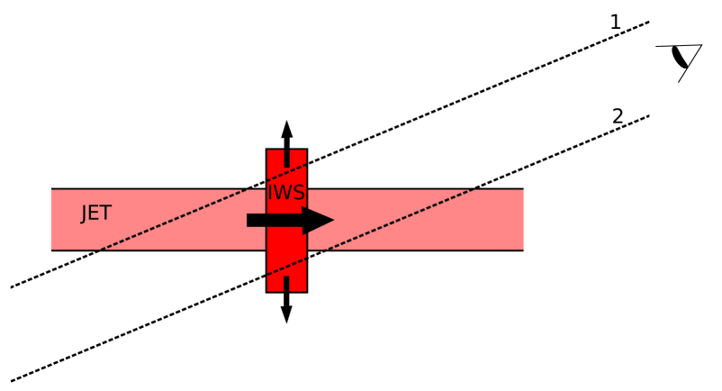
Figure 10: Schematic diagram showing how the sideways ejection of material in an internal working surface (IWS) makes the upstream gas appear faster than the downstream gas. In the upstream line of sight (labeled 1), the radial components of the jet motion (rightward arrow) and the sideways ejection (upward arrow) are both directed towards the observer and their contributions reinforce. In the downstream line of sight (labeled 2), the sideways ejection (downward arrow) contributes with the opposite sign to the radial velocity. Note that this effect does not rely on a specific orientation other than to increase or decrease the strength of the feature (as opposed to its sense).

If the teeth in the PV diagram represent lateral ejection of material from the IWSs, their width in velocity should be consistent with the observed broadening angle of the jet, which is determined by the ratio between the perpendicular and parallel components of the true velocity field (Landau & Lifshitz 1959). From the PV diagram in Fig. 9, we estimate that the (projected) mean jet velocity is 40 km s^-1, and that the sideways ejection velocity is about 5 km s^-1 (as each tooth has a width of about 10 km s^-1 in radial velocity). Thus, the ratio between the perpendicular and parallel components of the velocity field in the jet should be $5/40\cot\theta$, where $\theta$ is the the angle of the jet direction with the line of sight. Assuming $\theta=45^{\circ}$, the above ratio implies a jet full opening angle of $14^{\circ}$, which is in reasonable agreement with the $\approx 10^{\circ}$ measured from the CO(2–1) map in section 6.1. We thus conclude that the sawtooth pattern in the PV diagram corresponds to the sideways ejection of the post-shock gas in internal working surfaces.

6.3 CO versus SiO

Figures 3, 4, and 8 show that the EHV emission of CO(2–1) and SiO(2–1) have very similar spatial distributions and kinematic behavior. Discounting the factor-of-2 lower angular resolution of the SiO(2–1) data and the limited S/N of all maps, the EHV data of the two species seem compatible in all their main features. In particular, all the EHV peaks identified in CO(2–1) can be seen in SiO(2–1), especially when using maps with noise decreased by clipping, and the velocity pattern of the PV diagram is identical for both species. This similarity between the CO(2–1) and SiO(2–1) data is best understood if the two emissions trace the same gas component despite their potentially different excitation and chemical properties.

To further compare the CO(2–1) and SiO(2–1) emissions, we fit the distribution of EHV SiO(2–1) using the same 2D gaussian procedure used for CO(2–1). To ensure that the results for the two species are comparable, we force the SiO fit to use 2D gaussians with the same position and dimensions as those derived from CO(2–1), so the only free parameter in the SiO fit is the peak intensity. The results from this procedure, presented in Table 1, indicate that the ratio between the CO(2–1) and SiO(2–1) integrated intensities is close to 1 over the whole blue lobe, and that it ranges from 1 to 4 over the red lobe, having a trend to increase (i.e., SiO to weaken) with distance from the IRAS source. Without additional information from other transitions, assumptions on the molecular excitation are needed to convert the observed intensity ratio into a ratio of column densities. The detection of SiO(2–1), which has a critical density of about $4\;10^{5}$ cm^-3, suggests that the EHV gas is relatively dense, in agreement with previous analysis of similar EHV peaks in the L1448-mm outflow by Bachiller et al. (1991a) and Nisini et al. (2007). As these authors find that the density and temperature of the gas in the EHV peaks typically ranges between $10^{5}$-$10^{6}$ cm^-3 and 20-500 K (see also Hatchell et al. 1999), we have run a series of LVG radiative transfer models covering that range and determining the CO(2–1)/SiO(2–1) intensity ratio assuming optically thin emission. From this grid of models, we find that the conversion factor between the CO(2–1)/SiO(2–1) intensity ratio and the CO/SiO column density ratio is on average about 400, with an approximate factor of 2 variation in the range of expected densities and temperatures. We thus estimate that the CO/SiO abundance ratio in the EHV gas is close to 400, at least in the inner half of the jet. There is a possible increase of this ratio at large distances in the red lobe, but we cannot rule out that it is an effect of a density decrease in the outer EHV, as expected from the expansion of the gas, and as seen from a multi-line SiO analysis of the L1448-mm outflow by Nisini et al. (2007). Observations of additional SiO transitions in I04166 are clearly needed to clarify this issue.

SiO emission in outflows has usually been interpreted as resulting from the release of silicon atoms in the dust grains of the ambient cloud due to their shocking by the outflow primary wind (Caselli et al. 1997; Schilke et al. 1997). As discussed in the previous section, however, the kinematics of the EHV gas suggests that this outflow component is not shocked ambient material, but gas emitted in the form of a jet from the innermost vicinity of the central source, so the standard explanation for SiO production seems not to apply to this component. An alternative SiO formation mechanism that is more likely to apply to the EHV gas is the one presented by Glassgold et al. (1991), who have carried out simplified (1D) models of the chemistry of a primary wind from a low-mass protostar. These authors have shown that molecules can form efficiently via gas-phase reactions in an initially atomic protostellar wind, provided that the density and temperature of the wind stay within a range of appropriate values. CO, in particular, forms over a wide range of density conditions, and it tends to reach an equilibrium abundance of $4\;10^{-4}$, while SiO is more sensitive to density and to the possible presence of a photodissociating far-UV radiation field. Although the results from the Glassgold et al. (1991) model are not not fully comparable to our observations because the model assumes a luminosity of the central source that is two orders of magnitude higher than the 0.4 L_⊙ estimated for I04166 (and the model wind speed is probably a factor of two too high), they do provide an order of magnitude estimate of the expected chemistry in the EHV component. As mentioned previously, we estimate that the mass loss rate in the EHV component of I04166 is of the order of $5\;10^{-7}$ M_⊙ yr^-1, which is in the low range of values considered by Glassgold et al. (1991). For this mass loss rate, the models predict a substantial production of CO, and an abundance that depending on the details of the model can be as high as $10^{-5}$. The expected CO/SiO abundance ratio for this mass loss rate, however, is orders of magnitude lower than observed, although SiO formation is so sensitive to density that model predictions for a mass loss rate only ten times higher can easily match our observed CO/SiO ratio. Indeed, the gas density inside the jet-like EHV component of I04166 is likely to be higher than assumed by Glassgold et al. for their spherical models (even if these authors use a simple modification of the density law to simulate the effect of collimation), as the divergence of the spherical wind ends up dominating the density drop. In addition to this collimation effect, a further density enhancement occurs in the IWSs, and under appropriate conditions, this enhancement can lead to a higher rate of molecule formation (Raga et al. 2005). Thus, gas-phase production in the jet seems a viable mechanism for the formation of CO and SiO in the EHV gas. A further exploration of the chemistry of the EHV component and its comparison with the shock-dominated chemistry of the slower outflow material will be presented elsewhere (Santiago-García et al. 2008, in preparation).

7 Implications for outflow models

Our observations of I04166 show that jet-like and shell-like distributions of CO emission can be present simultaneously in a young bipolar outflow. Although not often emphasized, such a coexistence of jet and shell elements in the outflow material is not unique to I04166, and can be inferred in other outflows from Class 0 sources with a varying degree of detail depending on the angular resolution and signal-to-noise ratio of the observations. The outflow from L1448-mm, for example, has a jet-like EHV component first seen with single dish observations by Bachiller et al. (1990). Further higher angular resolution data of this outflow from the PdBI (Bachiller et al. 1995) have revealed that the low velocity outflow gas moves along two opposed shells, although these observations did not provide enough sensitivity to study in detail the EHV component and its relation to the shells. Recent observations of the L1448-mm outflow with the SMA by Jørgensen et al. (2007) confirm the presence of shells surrounding symmetrically the EHV component. Additional outflows where highly collimated jets of EHV gas coexist with quasi-conical shells of low velocity material include the one powered by IRAS 03282+3035, whose EHV jet was discovered by Bachiller et al. (1991b), and whose low velocity shells have been recently mapped with the OVRO interferometer by Arce & Sargent (2006). The HH211 outflow, observed with a number of interferometers (Gueth & Guilloteau 1999; Palau et al. 2006; Hirano et al. 2006; Lee et al. 2007), also presents a high velocity jet and a partially-surrounding low velocity shell. These and other observations suggest that EHV jets are often or always surrounded by lower velocity shells, although a systematic study of a larger sample of Class 0 outflows is still needed to confirm this conclusion. If the hypothesis is correct, the I04166 outflow should be considered as a particularly clean example of its class, probably due to its relatively close proximity and favorable orientation on the sky.

As discussed in the introduction, the presence of both jet-like and shell-like features in an outflow poses a problem to models that assume a simple geometry for the outflow driving agent. Neither models with only a jet-like component (e.g., Masson & Chernin 1993) nor wide-angle wind models (e.g., Shu et al. 1991) seem capable of explaining simultaneously the jet and shell features seen towards I04166 and similar objects. In order to reproduce these features, a model needs to include simultaneously a central jet and a surrounding wide-angle wind, both emerging from the very vicinity of the central embedded object. In recent years, a number of models with these characteristics have been presented in the literature, suggesting that two-component winds constitute a natural geometry for a protostellar outflow. Banerjee & Pudritz (2006) have carried out MHD simulations of a rotating core undergoing gravitational collapse and found an outflow consisting of an inner jet powered by magnetocentrifugal forces surrounded by a broad outflow driven by toroidal magnetic pressure. Unfortunately, these simulations only extend to 600 AU, which is not much larger than the resolution element of our observations. From a different MHD collapse simulation, Machida et al. (2008) also find a two-component outflow, this time consisting of a slow, wide-angle wind driven from the adiabatic (first) core which surrounds a faster, highly collimated jet driven from the protostar (or second core).

Although this geometry matches rather nicely the observations presented here, the outflow speeds predicted by these simulations ($\approx 5$ km s^-1 for the wide angle wind and $\approx 30$ km s^-1 for the jet) seem significantly lower than the values observed towards I04166 and similar outflows (the L1448-mm jet has an radial velocity of about 50 km s^-1, as measured by Bachiller et al. 1990).

An alternative model of an outflow with both jet-like and wide angle components is the “unified model” presented by Shang et al. (2006). These authors have carried out a numerical (Zeus2D) simulation of the interaction between a protostellar wind (based on the X-wind theory of Shu et al. 1994) and a density distribution expected for a magnetic dense core (Li & Shu 1996), and they have predicted the appearance of the resulting outflow-core system as a function of time. From these simulations, Shang et al. (2006) find that the gas distribution in each outflow lobe is dominated by a close-to-conical shell of low velocity gas and a highly collimated central jet of fast material, two features that bear remarkable similarities with those observed towards I04166. This resemblance between the predictions from the unified model and the I04166 observations is not only morphological, but kinematical, as both the jet and the shells have velocities close to those observed in Class 0 outflows. In addition, the shells in the unified model contain accelerated ambient gas with a strong longitudinal component, and the highly collimated jet represents the protostellar wind traveling at close to constant speed. These two characteristics agree with the properties derived in the previous sections for the shells and the jet of I04166, suggesting that the unified model captures at least some of the basic physics underlying the youngest bipolar outflows. The analysis of I04166 presented here, however, indicates that time variability in the fastest component and the resulting generation of IWSs along the jet are dominant effects in the observed molecular emission, so their inclusion in the simulations is still required to produce a realistic model of a bipolar outflow.

8 Summary

We have presented results from CO(2–1) and SiO(2–1) interferometer observations of the outflow powered by I04166, one of the youngest protostars in the Taurus molecular cloud. From the analysis of the geometry and kinematics of the emission, together with a comparison with existing models of outflow physics and chemistry, we have reached the following conclusions:

1. At a resolution of about 1.5 arcsec, the outflow seems powered by a single YSO whose disk (plus unresolved inner envelope) has a mass of 0.02 M_⊙.

2. The bipolar outflow is highly symmetric with respect to the position of I04166. Each outflow lobe consists of two separate and well-defined components. At radial velocities lower than 10 km s^-1, the gas lies along two opposed limb-brightened conical shells that have the YSO at their vertex and that have a full opening angle of 32 degrees. At radial velocities higher than 30 km s^-1, the gas forms a pair of highly collimated jets that emerge from the vicinity of the YSO and travel along the shell axis.

3. The geometry and kinematics of the low-velocity outflow shells are consistent with the gas being ambient cloud material that has been accelerated by a wide-angle wind. In agreement with this interpretation, we find that the northern blue shell coincides with the walls of an evacuated cavity seen as a reflection nebula in Spitzer NIR images.

4. The highly collimated jet shows no evidence for precession and consists of a symmetric collection of at least 7 pairs of intensity peaks. The peaks broaden with distance to I04166, and several of the outermost ones present shapes reminiscent of bow shocks. The full opening angle of the peaks is about 10 degrees, which is insufficient to explain the low velocity shells as a result of the sideways acceleration of the ambient gas by bow shocks in the jet. The mass loss rate estimated (with a large uncertainty) from this jet component is $5\times 10^{-7}$ M_⊙ yr^-1.

5. The velocity field of the collimated gas presents a sawtooth pattern that combines a close-to-constant mean velocity with internal gradients inside the emission peaks. In each emission peak, the gas closer to the YSO (tail) moves faster than the gas further away from it (head). The transition between these two speeds is almost linear, and it has a slope that flattens with distance to I04166. Such a velocity pattern is inconsistent with the emission peaks being solid bullets, collections of shrapnel, or shocked ambient gas. It is in good agreement with the predictions for internal working surfaces resulting from time variability in the outflow ejection speed. Variability in the central accretion may be responsible for these velocity changes in the outflow ejection. The time scale of this variability is of the order of 100 years.

6. The geometry and kinematics of the highly-collimated, fast gas suggests that this component consists of material emitted from the protostar or from its immediate vicinity, and not of swept up ambient gas. The relative abundance of CO and SiO that we derive for this component is in reasonable agreement with the chemical model of a protostellar wind presented by Glassgold et al. (1991).

7. The combination in a single outflow of low-velocity shells accelerated by a wide-angle wind and a fast, jet-like component moving along the shell axis illustrates the need for an outflow mechanism that produces these two different features simultaneously. The recent “unified” model of Shang et al. (2006) seems in good agreement with these characteristics, although the presence of internal working surfaces in the I04166 outflow indicates that time dependence in the ejection velocity is an additional element needed to model realistically outflow observations.