Solid-liquid coexistence of polydisperse fluids via simulation

Abstract

We describe a simulation method for the accurate study of the equilibrium freezing properties of polydisperse fluids under the experimentally relevant condition of fixed polydispersity. The approach is based on the phase switch Monte Carlo method of Wilding and Bruce [Phys. Rev. Lett. 85, 5138 (2000)]. This we have generalized to deal with particle size polydispersity by incorporating updates which alter the diameter $\sigma$ of a particle, under the control of a distribution of chemical potential differences $\tilde{\mu}(\sigma)$. Within the resulting isobaric semi-grand canonical ensemble, we detail how to adapt $\tilde{\mu}(\sigma)$ and the applied pressure such as to study coexistence, whilst ensuring that the ensemble averaged density distribution $\rho(\sigma)$ matches a fixed functional form. Results are presented for the effects of small degrees of polydispersity on the solid-liquid transition of soft spheres.

I Introduction and background

Our ability to accurately determine the phase coexistence properties of model systems via computer simulation has increased greatly in recent years. Progress has come in the form of specialized Monte Carlo methods that are tailor-made for tackling the core problem of coexistence, namely the comparison of the statistical weights of the disjoint regions of configuration space associated with competing phases. To achieve this one generally aims to engineer a sampling path which connects the phases in question, allowing each to be visited repeatedly in the course of a single simulation run. The reward for doing so comes in the form of direct, accurate and transparent measurements of free energy differences and coexistence parameters Bruce2003 .

In practice, however, the most obvious choice of an inter-phase sampling path, namely one routed via mixed-phase (ie. interfacial) configurations may not always be the most straightforward to negotiate. Typically such regions of configuration space are characterized by large free energy barriers, or by a ‘pitted’ free energy landscape – features which hinder efficient sampling. Contemporary strategies seek to either surmount or circumvent these impediments (for a review see Bruce2003 ). One such scheme – which is in principle rather general – is phase switch Monte Carlo (PSMC). Its key feature is a phase space ‘leap’ bruce2000 that directly maps a pure phase configuration of one phase onto a pure phase configuration of another. As such it completely avoids mixed-phase configurations and any attendant sampling difficulties.

In the context of fluid-solid coexistence, PSMC permits efficient two-phase sampling and hence the direct determination of equilibrium freezing parameters and their uncertainties. This contrasts with simulation approaches which seek to emulate physical crystal nucleation processes, which commonly encounter significant problems, principally a large degree of metastability of the phases, extended timescales for crystallization and a tendency for the crystals formed to exhibit vacancies, interstitials and other defects. To date, PSMC has been successfully applied to the freezing of hard spheres, softly repulsive spheres, and the Lennard-Jones fluid wilding2000 ; errington2004 ; mcneil-watson2006 ; Wilding2008 .

The present paper is concerned with extending the applicability of PSMC to the study of the freezing properties of model polydisperse fluids. Polydispersity is the feature, pervasive in soft condensed matter systems such as colloids and liquid crystals, whereby the constituent particles are not all identical but instead exhibit variation in terms of some attribute ($\sigma$, say) such as the particle size or shape, etc. It leads to phase behaviour that is considerably richer in both variety and form than that of monodisperse systems Sollich2002 .

Typically one describes the polydispersity of a given system in terms of a density distribution $\rho^{(0)}(\sigma)$ which counts the number of particles per unit volume having $\sigma$ in the range $\sigma\dots\sigma+d\sigma$. In most real polydisperse systems the form of $\rho^{(0)}(\sigma)$ is fixed by the synthesis of the fluid, and only its scale can change according to the degree of dilution of the system. Accordingly, one writes $\rho^{(0)}(\sigma)=n^{(0)}f(\sigma)$ where $f(\sigma)$ is a normalized fixed shape function and $n^{(0)}$ is the overall number density. Varying $n^{(0)}$ corresponds to scanning a “dilution line” of the system.

At coexistence, the particles of the various $\sigma$ values will be partitioned unequally between the phases. This is the phenomenon of “fractionation” which underpins the opulence of polydisperse phase behaviour. To describe fractionation it is necessary to define separate “daughter” distributions $\rho^{(i)}(\sigma)$ ( $i=1,2...$) which measure the distribution of the polydisperse attribute for each phase $i$. When the polydispersity is fixed, conservation of particles implies that the weighted average of the daughter distributions equals the fixed overall density distribution, or “parent” $\rho^{(0)}(\sigma)$, For instance, at two-phase coexistence $\rho^{(0)}(\sigma)=n^{(0)}f(\sigma)=(1-\xi)\rho^{(1)}(\sigma)+\xi\rho^{(2)}(\sigma)$, with $1-\xi$ and $\xi$ the respective fractional volumes of the phases. This expression represents a generalisation of the Lever rule to polydisperse systems.

To illustrate the central role of fractionation in polydisperse phase behaviour, it is constructive to consider first the familiar case of the binodal curve of a monodisperse system in the density-temperature plane. This curve serves a dual purpose: on the one hand it describes the range of overall densities for which phase coexistence occurs; and on the other hand it identifies the densities of the coexisting phases themselves. Now, for a polydisperse system the range of overall (parent) densities that leads to coexistence is similarly delineated by a curve in $n^{(0)}$-$T$ space – the so-called “cloud” curve. However, the densities of the coexisting phases themselves do not in general coincide with the cloud curve. Instead, as one varies the parent density $n^{(0)}$ through the coexistence region at a fixed temperature (say), one generates an infinite sequence of pairs of differently fractionated coexisting phases. It is customary to single out the end points of this sequence for special attention, ie. the case of incipient phase separation that occurs when the value of $n^{(0)}$ coincides with the cloud curve. Under these conditions, one daughter phase has a fractional volume of essentially unity and consequently (from the Lever rule) a density distribution that is identical to the parent, while the other phase – known as the “shadow” – has an infinitesimal fractional volume and a density distribution that deviates maximally from that of the parent. The curve formed by plotting the number density (or packing fraction) of the shadow phase as a function of temperature is known as the shadow curve.

Qualitative differences between the phase behaviour of monodisperse and polydisperse systems are also evident in other projections of the full phase diagram. For instance, in the pressure-temperature plane, coexistence for a monodisperse system occurs along a simple line. By contrast for a polydisperse system, coexistence occurs within a region of the pressure-temperature phase diagram Rascon2003 ; bellier-Castella2000 . Accordingly the task of exploring the full coexistence behaviour of a polydisperse system represents a far greater endeavor than for a monodisperse system.

Owing to the computational complexities associated with polydispersity, simulation studies of its effects on fluid-solid phase equilibria have been rather sparse. In pioneering work, Bolhuis and Kofke employed an isobaric semi-grand canonical ensemble approach to study the effects of particle size polydispersity on hard sphere freezing bolhuis1996b ; kofke1999 . Within this ensemble, Monte Carlo updates are performed that allow particles to change diameter, under the control of an imposed distribution of chemical potential differences $\tilde{\mu}(\sigma|\sigma_{0})=\mu(\sigma)-\mu(\sigma_{0})$, with $\sigma_{0}$ a reference particle diameter. The advantage of this approach is two fold: it allows the instantaneous form of the density distribution $\rho(\sigma)$ to fluctuate, thereby sampling many different realizations of the disorder in the course of a run, and it permits fractionation of the coexisting phases. However, in this early work no attempt was made to adapt the form of $\tilde{\mu}(\sigma)$ in order to ensure that the ensemble averaged density distribution $\bar{\rho}(\sigma)$ had a fixed functional form. Instead the activity distribution $\exp[\beta\tilde{\mu}(\sigma)]$ was assigned a Gaussian form, peaked at $\sigma_{0}$, and various widths of the Gaussian were studied in order to change the degree of polydispersity. In such a fixed chemical potential representation, $\bar{\rho}(\sigma)$ can vary dramatically across the phase diagram. Additionally, coexistence occurs only along a line in the $p-T$ plane (as in the monodisperse case), rather than within a region as occurs experimentally. These artifacts limit the applicability of the results.

To obtain the properties of the fluid-solid phase boundary, Bolhuis and Kofke employed Gibbs-Duhem integration (GDI) techniques. This approach traces a coexistence line in pressure-temperature space by integrating its derivatives, obtainable from measurements of single phase properties near coexistence. The principal strengths of GDI is that it can quickly yield an estimate for a phase boundary and avoids mixed phases configurations. However, independent prior knowledge of a coexistence state point is required in order to bootstrap the integration, and since there is no reconnection of the two phases beyond the initial starting point, integration errors can accumulate. The magnitude of these errors is difficult to quantify because there is no feedback mechanism to indicate when the integration has departed from the true coexistence line (provided one remains within the rather wide band of metastable states that borders this line).

In more recent simulation work, Fernández et al Fernandez2007 used a canonical ensemble approach to investigate the freezing of polydisperse soft spheres. However, owing to the small system size employed, the physical separation of the phases that would normally be expected to occur in a canonical ensemble simulation was (for the most part) absent and hence fractionation of the individual phases could not be measured. Consequently the “phase boundary” presented by Fernández et al contains no information on the properties of any of the infinity of coexisting fluid-solid pairs, serving at best only as a rough estimate of the middle of the range of parent densities for which coexistence might occur.

The method described in the present paper permits the accurate study of fluid-solid coexistence for systems of particles whose polydispersity is fixed. Accuracy is obtained by embedding the isobaric semi-grand canonical ensemble within the PSMC framework, thus allowing the direct connection of the coexisting phases. Fixed polydispersity is realized by implementing an iterative reweighting scheme that adapts $\tilde{\mu}(\sigma)$ and the pressure $p$ such that the conjugate density distribution $\bar{\rho}(\sigma)$ matches a prescribed parent form, even within the coexistence region. Our paper is arranged as follows. In sec. II we provide a summary of principal aspects of PSMC as applied to monodisperse systems, before proceeding to detail the extensions necessary to deal with polydispersity. Thereafter we describe how one can use the method to accurately determine fluid-solid coexistence properties for systems having fixed polydispersity. Finally we provide some illustrative results for a system of polydisperse soft spheres, obtaining cloud points, demonstrating the broadening of the coexistence region in the pressure-temperature plane, and quantifying fractionation effects.

II Phase switch Monte Carlo

A full description of the statistical mechanical background to PSMC as well as an in-depth discussion of its implementation for problems of fluid-solid coexistence has recently been given elsewhere (see ref. mcneil-watson2006 ) and shall not therefore be repeated here in full. Instead we shall focus somewhat more on the generalities of the method, as a prelude to describing the extensions required to deal with polydispersity.

II.1 Monodisperse systems

Let us work within an isobaric-isothermal (constant-NpT) ensemble, in which the particle number $N$, pressure $p$ and temperature $T$ are all prescribed FrenkelSmit2002 . Then the relative stability of fluid (F) and crystalline solid (CS) phases is determined by the difference in their Gibbs free energies. This can in turn be obtained from the ratio of the a-priori probabilities of the phases Bruce2003 ; mcneil-watson2006 :

$$\Delta g\equiv g_{CS}(N,p,T)-g_{F}(N,p,T)\equiv\frac{1}{N}\ln{\mathcal{R}}_{\mbox{\sc{f,cs}}}\>.$$ (1)

with

$${\mathcal{R}}_{\mbox{\sc{f,cs}}}\equiv\frac{P(F|N,p,T)}{P(CS|N,p,T)}\>.$$ (2)

In order to directly measure ${\mathcal{R}}_{\mbox{\sc{f,cs}}}$, a MC procedure is required that samples both the solid and the fluid regions of configuration space in the course of a single simulation run at the prescribed values of $N,p$ and $T$. From this one simply measures the probabilities $P(F)$ and $P(CS)$ of finding the system in each of the respective phases, and thence the probability ratio. Below we describe how PSMC facilitates such a measurement.

PSMC takes as its starting point the specification of a reference configuration $\{\vec{R}\}^{\gamma}$ for each of the phases (labeled $\gamma$) coexisting at the phase boundary. The specific choice of $\{\vec{R}\}^{\gamma}$ is arbitrary, the only condition being that it should be a member of the set of pure phase configurations identifiable as “belonging” to phase $\gamma$. For a crystalline phase, a suitably simple choice of $\{\vec{R}\}^{CS}$ is the set of lattice sites; for a fluid, a suitable choice is a randomly chosen fluid configuration.

The next step is to express the coordinates of each particle in phase $\gamma$ in terms of the displacement from its reference site, i.e.

$$\vec{r}^{\gamma}_{i}=\vec{R}^{\gamma}_{i}+\vec{u}_{i}\>.$$ (3)

Now, for displacement vectors that are sufficiently small in magnitude, one can clearly reversibly map any configuration $\{\vec{r}^{\gamma}\}$ of phase $\gamma$ onto a configuration of another phase $\gamma^{\prime}$ simply by switching the set of reference sites $\{\vec{R}\}^{\gamma}\to\{\vec{R}\}^{\gamma^{\prime}}$, while holding the set of displacements $\{\vec{u}\}$ constant. This switch, which forms the heart of the method, can be incorporated in a global MC move (see fig. 1).

Figure 1: Schematic illustration of the phase switch mechanism. The dots identify the representative sites $\{\vec{R}\}^{\gamma}$ in each phase; the displacement vectors $\{\vec{u}\}$ connect the centers of the distinguishable (numbered) particles to these sites. The switch operation shown swaps the representative sites of one phase for those of the other phase, whilst maintaining $\{\vec{u}\}$ constant. The particular configuration $\{\vec{u}\}$ shown is a “gateway” state (see text) because the magnitude of the effective energy change under the switch is small.

A complication arises however, because the displacements $\{\vec{u}\}$ typical for phase $\gamma$ will not, in general, be typical for phase $\gamma^{\prime}$. Thus the switch operation will mainly propose high energy configurations of phase $\gamma^{\prime}$ which are unlikely to be accepted as a Metropolis update. This problem can be circumvented by employing extended sampling (biasing) techniques to seek out those displacements $\{\vec{u}\}$ for which the switch operation is energetically favorable. These are the gateway configurations, which typically correspond to displacement vectors which are small in magnitude. Fig. 2 shows a schematic representation of the procedure.

Figure 2: Schematic illustration of the phase switch operation in terms of the regions of configuration space associated with the fluid and crystalline solid phases. A bias (dashed arrows) is constructed such as to enhance the probability of the subsets of “gateway” states (the white islands) within the single-phase regions, from which the switch operation (the large arrow) will be accepted. Note that the switch accesses only one of the crystalline phase space replica fragments associated with permutations of particles amongst lattice sites mcneil-watson2006 .

The requisite bias is administered with respect to an “order parameter” $M$. This macrovariable is defined such that the set of typical microstates (particle configurations) associated with its range, form a continuous phase space path linking the configurations of high statistical weight to the gateway configurations. In our formulation, the order parameter comes in two parts (or modes): ‘tether’ and ‘energy’. The tether mode serves to draw particles close to the representative sites to which they are nominally associated. Then, once all particles are within a prescribed distance of these sites, tether mode switches off and an energy mode order parameter takes over to guide particle to the gateway states for which the phase switch energy cost is sufficiently small to be accepted.

To elaborate, let $M_{m,\gamma}$ denote the order parameter in mode $m$ and phase $\gamma$. Then for tether mode we write $m={\cal T}$ and define an associated order parameter

$$M_{{\cal T},\gamma}(\{\vec{u}\})=\left(\frac{1}{N}\sum_{i=1}^{N}{\rm max}\{0,\tilde{u}_{i}-\tilde{u_{c}}\}\right)^{1/2}\>,$$ (4)

where $\tilde{u}_{i}=|{\bf u}_{i}|/V^{1/3}$ is the distance of particle $i$ from its lattice site measured in units of the box length, and $\tilde{u_{c}}$ is a prescribed dimensionless threshold radius. Only particles whose displacement $\tilde{u}_{i}$ exceeds this threshold contribute to $M_{{\cal T},\gamma}$.

The tether mode is active iff $\tilde{u}_{i}>\tilde{u_{c}}\>$ for at least one particle $i$, i.e. when $M_{{\cal T},\gamma}>0$. Otherwise control hands over to the ‘energy’ mode $m={\cal E}$; its associated order parameter is defined by

$$M_{{\cal E},\gamma}(\{\vec{u}\})=\mathrm{sgn}(\Delta{\cal E}_{\gamma^{\prime}\gamma})\ln(1+|\Delta{\cal E}_{\gamma^{\prime}\gamma}|)\>,$$ (5)

where

$$\Delta{\cal E}_{\gamma^{\prime}\gamma}=({\cal E}_{\gamma}-{\cal E}^{\rm ref}_{\gamma})-({\cal E}_{\gamma^{\prime}}-{\cal E}^{\rm ref}_{\gamma^{\prime}})$$ (6)

measures the change (under the phase switch operation) of the enthalpy ${\cal E}_{\gamma}(\{\vec{u}\},V)=\Phi_{\gamma}(\{\vec{u}\})+pV$ with respect to its value ${\cal E}^{\rm ref}$ in the representative microstate $\{\vec{R}\}^{\gamma}$, with the latter scaled to the instantaneous volume of phase $\gamma$ Jackson2002 ; errington2004 . The presence of the logarithm in eq. 5 is designed to moderate the scale of the contribution of the energy cost to $M_{{\cal E},\gamma}$, which might otherwise become excessively large for particles with a strongly repulsive core to their interaction potential.

Having defined a suitable order parameter, a biasing (weight) function is constructed to allow the system to reach the gateway states and hence – in the course of a sufficiently long run – switch back and forth repeatedly from fluid to solid. This weight function comes in four parts, one for each combination of phase and mode, and the interface between energy and tether parts are joined for continuity at their boundary. A number of techniques exist for constructing this weight function, but of those we have tested, we have found transition matrix Monte Carlo Smith1995 to be (by far) the most efficient. Details of how to implement the transition matrix approach to obtain the weight function in the context of PSMC have previously been described elsewhere errington2004 ; mcneil-watson2006 and we refer the interested reader to those articles for details.

Turning now to the Monte Carlo procedure for sampling the order parameter distribution, in the context of monodisperse systems this involves four types of update, as outlined below.

1. ‘Particle translations’. A site (identified by one of the vectors in $\{\vec{R}\}^{CS}$ or $\{\vec{R}\}^{F}$) is selected at random and a candidate state is chosen by incrementing the position coordinate of the particle associated with that site by a random vector whose components are drawn from a zero-mean uniform distribution of prescribed width. This operation changes both $\{\vec{r}\}$ and $\{\vec{u}\}$

2. ‘Association swaps’. In this operation we choose two distinct sites at random ($i$ and $j$ say) and identify the corresponding displacement vectors $\vec{u}_{i}$ and $\vec{u}_{j}$. The candidate state is defined by the replacements

   $$\vec{u}_{i} \rightarrow \vec{u}_{j}+\vec{R}_{j}-\vec{R}_{i}$$ (7)

   $$\vec{u}_{j} \rightarrow \vec{u}_{i}+\vec{R}_{i}-\vec{R}_{j}$$ (8)

   This process can be regarded as a change of association: the particle which was associated with site $j$ is now associated with site $i$ (and vice versa). It changes the representation of the configuration (the coordinates $\{\vec{u}\}$); but it leaves the physical configuration invariant. It need be applied only to the fluid phase where particles can wander far from their representative sites and need to be reined back in order to reach the gateway states.

3. ‘Volume moves’. The volume is also updated in the conventional way FrenkelSmit2002 , by a random walk of prescribed maximum step size, with particle position coordinates $\{\bf{r}\}$ and representative sites $\{\vec{R}\}^{\gamma}$ rescaled.

4. ‘Inter-phase switch’. The final type of MC update is the phase switch, which entails replacing one set of the representative configuration vectors, $\{\vec{R}\}^{\gamma}$ say, by the other, $\{\vec{R}\}^{\gamma^{\prime}}$. The switch should also incorporate an appropriate volume scaling of the system.

Details of the appropriate biased acceptance probabilities for these moves can be found in the original articles wilding2000 ; mcneil-watson2006 .

Using these MC updates, together with a suitable estimate of the weight function, the sampling process can be initiated. During this process one accumulates (initially in the form of a list wilding2001 ) the joint probability distribution of the order parameter, the volume, the energy and the phase label $\gamma$. Subsequently the effects of the imposed bias are unfolded from this distribution (in the standard manner Bruce2003 ; wilding2000 ; mcneil-watson2006 ) to provide a direct measure of the relative probabilities of the two phases:

$${\mathcal{R}}_{\mbox{\sc{f,cs}}}=\frac{\int dM\;dV\;d{\cal E}\;P(M,V,{\cal E},F)}{\int dM\;dV\;d{\cal E}\;P(M,V,{\cal E},CS)}\>,$$ (9)

from which the Gibbs free-energy-density difference follows directly via Eqs. 1 and 2. In practice these integrals are estimated by simple sums over the list of sampled values of $M,V,{\cal E},\gamma$. Use of histogram reweighting (HR) ferrenberg1989 permits exploration of values of the $p$ and $T$ in the neighbourhood of a given simulation state point and serves as an invaluable aid for pinpointing the coexistence parameters at which the free energy difference vanishes.

II.2 Extension to polydisperse systems

The natural choice of simulation ensemble for the study of $F$-$CS$ coexistence in polydisperse systems is the isobaric, semi-grand-canonical ensemble Kofke1988 . Within this ensemble, the particle number $N$, pressure $p$, temperature $T$, and a distribution of chemical potential differences $\tilde{\mu}(\sigma|\sigma_{0})$ are all prescribed, while the system volume $V$, the energy, and the form of the instantaneous density distribution $\rho(\sigma)$ all fluctuate. The fluctuation in $\rho(\sigma)$, although subject to the constraint $V\int\rho(\sigma)d\sigma=N$, nevertheless permits the sampling of many realizations of the polydisperse disorder, thus ameliorating finite-size effects. Moreover, in conjunction with volume fluctuations, it facilitates separation into differently fractionated phases.

Operationally, the sole difference between the isobaric, semi-grand-canonical ensemble and the constant-NpT ensemble used for PSMC is that one implements MC updates that select a particle at random and attempt to change its diameter $\sigma$ by a random amount drawn from a zero-mean uniform distribution. This proposal is accepted or rejected with a Metropolis probability controlled by the change in the internal energy and chemical potential Kofke1988 :

$$p_{\rm acc}={\rm min}\left[1,\exp{(-\beta[\Delta\Phi+\tilde{\mu}(\sigma)-\tilde{\mu}(\sigma^{\prime})])}\right]\>,$$

where $\Delta\Phi$ is the internal energy change associated with the resizing operation. Accordingly, one can readily extend the PSMC framework to deal with polydispersity by specifying a form for $\tilde{\mu}(\sigma|\sigma_{0})$ and supplementing the four Monte Carlo operations described in Sec. II.1 with a resizing move. For the purposes of histogram reweighting, one samples the joint probability distribution of the order parameter, the volume, the energy and the instantaneous density distribution $\rho(\sigma)$. Again this can be conveniently stored as a simple list of sampled values.

III Fixed polydispersity

For simulations of fixed polydispersity at some given $N$ and $T$, one requires that both the pressure $p$ and $\tilde{\mu}(\sigma)$ are such that a suitably defined ensemble-averaged density distribution matches the prescribed parent $\rho^{(0)}(\sigma)=n^{(0)}f(\sigma)$. Unfortunately, the task of determining the requisite $p$ and $\tilde{\mu}(\sigma)$ is severely complicated by the fact they are an unknown functional of the parent. Essentially, therefore, one is faced with solving an inverse problem wilding2003a .

To deal with this problem we employ a scheme similar to one recently proposed in the context of grand canonical ensemble studies of polydisperse phase coexistence buzzacchi2006 . The method relies on the fact that data accumulated at a given set of $p$ and $\tilde{\mu}(\sigma)$ can be used to extrapolate (via histogram reweighting) to other nearby sets of $p$ and $\tilde{\mu}(\sigma)$, without further simulation. In our description we shall assume for convenience that while the particle size $\sigma$ is to be treated as a continuous variable, distributions defined on $\sigma$, such as $\rho(\sigma)$, and $\tilde{\mu}(\sigma)$, are represented as histograms formed by discretising the range of $\sigma$ into a finite number of bins.

One proceeds as follows. The first step is to decide which of the infinity of coexisting pairs of phases inside the cloud curve one would like to determine for a given temperature $T$. To do so one specifies a value for the parameter $\xi$ which measures the fractional volume of the solid phase, and thus parameterizes the dilution lines between the liquid phase cloud ($\xi=0$) and the solid phase cloud ($\xi=1$). The general strategy for determining the coexistence properties at the given $\xi$ (and $T$) is then to tune $p,\tilde{\mu}(\sigma)$ and $n^{(0)}$ iteratively, such as to simultaneously satisfy both a generalized lever rule and equality of the a-priori probabilities of the phases, ie.

$$n^{(0)}f^{(0)}(\sigma) = (1-\xi)\rho^{(1)}(\sigma)+\xi\rho^{(2)}(\sigma)\>,$$ (10a)

$${\mathcal{R}}_{\mbox{\sc{f,cs}}} = 1\>.$$ (10b)

In the first of these constraints (Eq. 10a), the ensemble averaged daughter density distributions $\rho^{(1)}(\sigma)$ and $\rho^{(2)}(\sigma)$ are assigned by averaging only over configurations belonging to the fluid and solid phases respectively. The deviation of the weighted sum of the daughter distributions $\bar{\rho}(\sigma)\equiv(1-\xi)\rho^{(1)}(\sigma)+\xi\rho^{(2)}(\sigma)$ from the target $n^{(0)}f^{(0)}(\sigma)$ is conveniently quantified by a ‘cost’ value:

$$\Delta\equiv\int\mid\bar{\rho}(\sigma)-n^{(0)}f^{(0)}(\sigma)\mid d\sigma\;.$$ (11)

Requiring ${\mathcal{R}}_{\mbox{\sc{f,cs}}}=1$ in the second constraint (Eq. 10b), ensures that finite-size errors in coexistence parameters are exponentially small in the system volume  borgs1992 ; buzzacchi2006 .

The iterative determination of $p,\tilde{\mu}(\sigma)$ and $n^{(0)}$ such as to satisfy Eqs. 10a and 10b then proceeds thus:

1. Guess an initial value of the parent density $n^{(0)}$ corresponding to the chosen value of $\xi$. (If one starts with a small degree of polydispersity, a suitable estimate can be obtained from the densities of the coexisting phases in the known monodisperse limit, together with the lever rule.)

2. Tune the pressure $p$ (within the HR scheme) such as to minimize $\Delta$.

3. Similarly tune $\tilde{\mu}(\sigma)$ (within the HR scheme, see below) such as to minimize $\Delta$.

4. Repeat steps 2 and 3 until $\Delta<{\rm Tolerance}$.

5. Measure the corresponding value of ${\mathcal{R}}_{\mbox{\sc{f,cs}}}$.

6. if $|{\mathcal{R}}_{\mbox{\sc{f,cs}}}-1|<{\rm Tolerance}$, finish, otherwise vary $n^{(0)}$ and repeat from step 2.

The minimization of $\Delta$ with respect to variations in $p$ (step 2) can be easily automated using standard 1-dimensional minimization algorithms such as the “brent” routine described in Numerical Recipes Numericalrecipes . The same applies to the minimization of $|{\mathcal{R}}_{\mbox{\sc{f,cs}}}-1|$ with respect to variations in $n^{(0)}$ in step $6$. In step 3 the minimization of $\Delta$ with respect to variations in $\tilde{\mu}(\sigma)$ is most readily achieved wilding2002d using the following simple iterative scheme for $\tilde{\mu}(\sigma)$:

$$\tilde{\mu}_{k+1}(\sigma)=\tilde{\mu}_{k}(\sigma)+\alpha\ln\left(\frac{n^{(0)}f^{(0)}(\sigma)}{\bar{\rho}(\sigma)}\right)\;,$$ (12)

for iteration $k\to k+1$. This update is applied simultaneously to all entries in the histogram of $\tilde{\mu}(\sigma)$, and thereafter the distribution is shifted so that $\tilde{\mu}(\sigma_{0})=0$. The quantity $0<\alpha<1$ appearing in eq. 12 is a damping factor, the value of which may be tuned to optimize the rate of convergence.

In practice we find that the minimization of $\Delta$ with respect to variations in $\tilde{\mu}(\sigma)$ operates well provided $\bar{\rho}(\sigma)$ is sufficiently close to $n^{(0)}f^{(0)}(\sigma)$ for histogram reweighting to be effective. Note that (as described in buzzacchi2006 ) it is important that in steps $4$ and $6$, one iterates to a very high tolerance in order to ensure that the finite-size effects are exponentially small in the system size. Typically we iterated until both $\Delta$ and $|{\mathcal{R}}_{\mbox{\sc{f,cs}}}-1|$ were less than $10^{-12}$.

The values of $n^{(0)}$ and $p$ resulting from the application of the above procedure are the desired parent density and pressure corresponding to the nominated value of $\xi$. For $\xi=0$ and $\xi=1$, these are (respectively) the liquid and solid cloud point densities and pressures, while shadow points are given by the properties of the coexisting incipient daughter phase, which may be simply read off from the appropriate peak positions of the cloud point distributions of quantities such as the fluctuating packing fraction.

Finally in this section, we note that whilst in the interests of clarity we have not included a description of temperature reweighting in our procedure, it is straightforward to incorporate such. Doing so allows one to scan the $p-T$ plane in a stepwise fashion, and thus, ultimately, determine the entire transition region.

IV Solid-fluid coexistence of size-disperse soft spheres

We have applied our methodology to obtain the cloud and shadow point properties of a polydisperse system of softly repulsive spheres described by the $r^{-12}$ potential

$$v(r)=\epsilon(\sigma_{ij}/r)^{12}\>,$$ (13)

with $\sigma_{ij}=(\sigma_{i}+\sigma_{j})/2$. In fact, for a given choice of $f(\sigma)$ the thermodynamic state of this model does not depend on $n^{(0)}$ and $T$ separately but only on the combination $n^{(0)}(\epsilon/k_{B}T)^{1/4}$. Thus, the coexistence points for various temperatures scale exactly onto one another Hoover1970 and one therefore only needs to determine coexistence properties for a single temperature. Accordingly in this work we shall consider the case $(\epsilon/k_{B}T)=1$.

In our simulations, the interparticle potential was truncated at half the box size and periodic boundary conditions were applied. Since for the system sizes studied the value of the potential is extremely small at the typical cutoff radius, no correction was applied for the truncation.

We chose to study a parent distribution of the top-hat form defined by

$$f(\sigma)=\left\{\begin{array}[]{ll}(2c)^{-1}&\mbox{ if $1-c\leq\sigma\leq 1+c$}\\ ~{}~{}0&\mbox{ otherwise }\end{array}\right.,$$ (14)

where (without loss of generality), the mean particle diameter has been set to $\bar{\sigma}=1.0$. In this initial study we report results for a system of $N=256$ particles and rather narrow parent distributions $c\leq 0.05$, for which the dimensionless degree of polydispersity (ratio of standard deviation to mean of $f(\sigma)$ is $\delta=c/\sqrt{3}\lesssim 3\%$. For the purposes of forming $\tilde{\mu}(\sigma)$ and $\rho(\sigma)$, each unit of $\sigma$ was discretized into $500$ bins.

As a preliminary step we determined the coexistence parameters of the transition from fluid to face-centred-cubic (fcc) solid in the monodisperse limit. This was done using the standard formulation of PSMC (see sec. II.1) with the results Wilding2008 : $p_{coex}=22.32(3),\rho_{F}=1.148(9),\rho_{CS}=1.190(9)$. Thereafter we attempted to locate the fluid phase cloud point ($\xi=0$) for a narrow top-hat parent having $c=0.01$. To this end we initialized the chemical potential difference distribution as $\tilde{\mu}(\sigma)=0$ (for $0.99\leq\sigma\leq 1.01$) and $\tilde{\mu}(\sigma)=-100$ otherwise, and assigned the pressure the value $p=22.32$ pertaining to the monodisperse limit. We then performed a long PSMC run, the results of which were reweighted (using the procedure described in Sec. III together with the monodisperse value $n^{(0)}=1.148$ as the initial guess for the fluid cloud point density), to yield accurate estimates of the fluid phase cloud point pressure, parent density $n^{(0)}$ and chemical potential difference distribution $\tilde{\mu}(\sigma)$, as well as the shadow phase daughter distribution.

In order to progress to higher degrees of polydispersity, we proceeded in a stepwise fashion. The form of $\tilde{\mu}(\sigma)$ previously determined for $c=0.01$ was extrapolated via a quadratic fit to cover the range $0.98\leq\sigma\leq 1.02$, while the pressure for $c=0.02$ was estimated by linearly extrapolating the results for $c=0.00$ and $c=0.01$. A new PSMC run was then performed, the results of which were reweighted to give accurate estimates of the cloud point parameters for the top hat parent having $c=0.02$. In this manner we were able to steadily increase the degree of polydispersity, measuring the cloud point pressure and parent density as we went. In an identical fashion we determined the dependence on polydispersity of the solid cloud point parameters, by setting $\xi=1$ in the above procedure.

$c$	$p_{F}$	$n^{(0)}_{F}$	$p_{CS}$	$n^{(0)}_{CS}$
0	22.32(3)	1.148(9)	22.32(3)	1.190(9)
0.02	22.46(3)	1.149(1)	22.49(3)	1.192(2)
0.05	23.21(4)	1.159(1)	23.39(5)	1.201(2)

Table 1: Estimates of the coexistence pressure and parent density at the fluid and fcc-solid cloud points for the half-widths $c$ of the top-hat parent distribution indicated.

Table. 1 shows the fluid and solid cloud point parameters for $c=0,0.02$ and $0.05$. We note that our results for the monodisperse limit ($c=0$) are consistent with existing estimates for the same model obtained via thermodynamic integration Hoover1970 . Our data for $c>0$ exhibit a clear separation of the cloud point pressures as polydispersity increases, reflecting the polydispersity-induced broadening of the coexistence region described in Sec. I. Also apparent is an increase in the cloud point densities with increasing polydispersity, a finding which is in accord with theoretical predictions for polydisperse hard spheres fasolo2004 . In Fig. 3 we plot the form of the shadow phase daughter distributions for $c=0.05$. This shows that at the fluid phase cloud point the incipient solid phase contains a majority of large particles compared to the parent, whilst at the solid phase cloud point, the incipient (liquid) phase contains a majority of small particles. This too is in accord with the predictions for models of polydisperse hard spheres fasolo2004 . Fig. 3(b) shows the corresponding cloud point forms of the chemical potential difference distribution $\tilde{\mu}(\sigma)$.

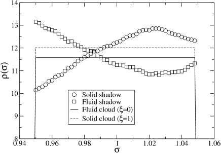
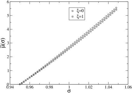
Figure 3: (a) Estimates of the cloud and shadow point density distributions for $c=0.05$. (b) Corresponding distribution of chemical potential differences, for $\sigma_{0}=0.95$. Statistical uncertainties do not exceed the symbol sizes.

Finally, we consider how one obtains the properties of shadow phases such as their average packing fraction or average number density. This is illustrated in Fig. 4 which shows (for $c=0.05$) the form of the probability distribution of the fluctuating packing fraction at the solid cloud point ($\xi=1$), ie. the distributions $P(\eta^{(1)})$ and $P(\eta^{(2)})$ with $\eta^{(i)}=(\pi/6)\int\sigma^{3}\rho^{(i)}(\sigma)$. The peak at large $\eta$ corresponds to the solid cloud phase and the peak at lower $\eta$ corresponds to the fluid shadow phase. The average of the shadow point packing fraction $\bar{\eta}$ can be simply read off from the position of the shadow phase peak. For a system with a non-trivial temperature dependence of the phase boundary, such plots (and analogous one for the number density), obtained for a range of temperatures, allow construction of the shadow curve in either the packing fraction or number density representation.

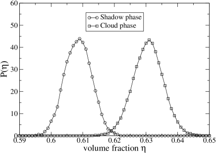
Figure 4: The distribution of the fluctuating packing fraction $P(\eta)$ in the solid cloud phase and in the shadow daughter phase for $c=0.05$, as described in the text. Statistical uncertainties are comparable with the symbol sizes.

V Conclusions

In summary, we have presented an accurate approach for determining the fluid-solid coexistence properties of polydisperse fluids under the experimentally relevant constraint that the parent distribution has a fixed functional form. The method is capable of determining the properties of any of the infinity of coexistence state points that pertain inside the cloud curve. By illustration we have determined the cloud and shadow properties at the freezing transition for a system of soft spheres having small degrees of polydispersity.

Like the bare PSMC method on which it is based, our approach requires a significant investment of computational effort in order to reap the benefits of accurate estimates of coexistence properties. The results presented here required about $4$ weeks of CPU time on an 8-core, 3GHz processor. Nevertheless, it should be straightforward to extend our study to higher degrees of polydispersity and larger system sizes, albeit with a correspondingly increased computational expenditure.

Thus our method could prove useful in helping to investigate interesting theoretical predictions fasolo2004 concerning the fluid-solid coexistence properties of polydisperse fluids. Specifically, it has been proposed that while on the fluid cloud curve the degree of polydispersity of the fluid parent can be increased to rather large values of $\delta\gtrsim 14\%$, in the coexisting (shadow) solid daughter phase, $\delta$ never exceeds the more modest value $\delta\approx 6\%$. On the other hand, on the solid phase cloud curve, the single solid parent is itself predicted to become unstable at about $\delta\approx 6\%$ and phase separates at a triple point into two solid phases and a liquid. We hope to be able to address these issues in future work.

- (1) A.D. Bruce and N.B. Wilding, Adv. Chem. Phys 127, 1 (2003).
- (2) AD Bruce, AN Jackson, GJ Ackland, and N.B. Wilding, Phys. Rev. E. 61, 906 (2000).
- (3) N.B. Wilding and A.D Bruce, Phys. Rev. Lett. 85, 5138 (2000).
- (4) J.R. Errington, J. Chem. Phys. 120, 3030 (2004).
- (5) G.C. McNeil-Watson and N.B. Wilding, J. Chem. Phys. 124, 064504 (2006).
- (6) N.B. Wilding, Mol. Phys. unpublished (2008).
- (7) P. Sollich, J. Phys.: Condens. Matter 14, R79 (2002).
- (8) C. Rascon and M.E. Cates, J. Chem. Phys. 118, 4312 (2003).
- (9) L Bellier-Castella, H Xu, and M Baus, J. Chem. Phys. 113, 8337 (2000).
- (10) PG Bolhuis and DA Kofke, Phys. Rev. E. 54, 634 (1996).
- (11) DA Kofke and PG Bolhuis, Phys. Rev. E. 59, 618 (1999).
- (12) L.A. Fernández, V. Martín-Mayor, and P. Verrocchio, Phys. Rev. Lett. 98, 085702 (2007).
- (13) D. Frenkel and B. Smit, Understanding Molecular Simulation (Academic, San Diego, 2002).
- (14) AN Jackson, AD Bruce, and GJ Ackland, Phys. Rev. E. 65, 036710 (2002).
- (15) G.R. Smith and A.D. Bruce, J. Phys. A 28, 6623 (1995).
- (16) N.B. Wilding, Am. J. Phys. 69, 1147 (2001).
- (17) A.M. Ferrenberg and R.H. Swendsen, Phys. Rev. Lett. 63, 1195 (1989).
- (18) D. A. Kofke and E.D. Glandt, Mol. Phys. 64, 1105 (1988).
- (19) N.B. Wilding, J. Chem. Phys. 119, 12163 (2003).
- (20) M. Buzzacchi, P. Sollich, N.B. Wilding, and M. Müller, Phys. Rev. E. 73, 046110 (2006).
- (21) C. Borgs and R. Kotecky, Phys. Rev. Lett. 68, 1734 (1992).
- (22) W.H. Press amd S.A. Teukolsky, W.T. Vetterling, and B.P. Flannery, Numerical Recipes (Cambridge University Press, Cambridge, 2007).
- (23) N.B. Wilding and P Sollich, J. Chem. Phys. 116, 7116 (2002).
- (24) W.G. Hoover et al., J. Chem. Phys. 52, 4931 (1970).
- (25) M Fasolo and P Sollich, Phys. Rev. E. 70, 041410 (2004).