Mesoscopic oscillator in U-shape with giant persistent current

Abstract

A mesoscopic oscillator in U-shape has been proposed and studied. Making use of a magnetic flux together with a potential of confinement, the electron contained in the oscillator has been localized initially and an amount of energy has been thereby stored. Then a sudden cancellation of both the potential and the flux may cause an initial current which initiates a periodic motion of the electron from one end of the U-oscillator to the opposite end, and repeatedly. The period is adjustable. The current associated with the periodic motion can be tuned very strong (say, more than two orders larger than the current of the usual Aharonov-Bohm oscillation). Related theory and numerical results are presented.

Due to the great progress in experiments, a few given number of electrons can be captured and confined in various ingenious artificial mesoscopic devices (say, quantum dots, wires, rings, and more complicated coupled dots, Mobius rings, etc.) r_LA98 ; r_LA2K ; r_HP ; r_KUF ; r_MD ; r_FA ; r_HEA ; r_VS . These devices are basic elements in micro-industry. In developing micro-techniques a crucial point is the counting of time. In this paper a micro-oscillator in U-shape is proposed, which might work as a mesoscopic pendulum.

It is recalled that, for classical motion, the crucial point of an oscillator is the storage of an amount of energy which can be transformed to kinetic energy later. For the classical pendulum, an amount of potential energy from gravity has been stored in advance, and will be transformed to the energy of swinging afterward. For a quantum oscillator, the crucial point is also how to store the energy. For this purpose, based on the idea suggested in the ref. r_HYZ , a device is proposed as sketched in Fig.1. The device is a ring together with two arms (AB and DE), wherein a few free electrons are contained. Previously, the arms are exactly blocked (say, by electrodes with high voltage), the ring is threaded by a magnetic flux $\Phi$, and a strong potential $V$ is applied so that the electron is localized in the bottom of the ring (close to point C in Fig.1a). In this way, an amount of energy (which can be quite large) has been stored as shown later. Suddenly, both $\Phi$ and $V$ are cancelled, and the block on the arms is released. Instead, the upper half circle of the ring is blocked. With this sudden change, the ring is transformed to a U-oscillator (Fig.1b). The previously stored energy will motivate an oscillation of the electrons, as we shall see, from one end (A) to the other end (E). Dissipation is assumed to be negligible (namely, a superconducting device). Then, the oscillation will proceed on in an exact periodic way. Related theories together with numerical results are as follows.

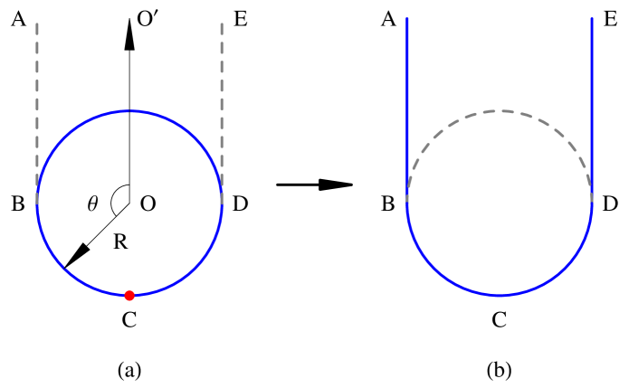
Figure 1: (Color online.) A sketch of the oscillator. The device in (a) is in fact a ring, where the two arms (AB and DE in dash line) are blocked. Whereas in (b) the upper half circle (in dash line) is blocked and the previous block on the arms is released. Thereby the ring is transformed to a U-pipe.

For simplicity, it is assumed that only one free electron with an effective mass $m^{*}$ is contained in the device. Let the radius of the ring be $R$ and the lengths of both arms be $l$. The ring and arms are very narrow so that they are quasi-one-dimensional. Previously, the Hamiltonian defined on the ring associated with Fig.1a reads

$$H_{init}=G(-i\frac{\partial}{\partial\theta}+\Phi)^{2}+V(\theta)$$ (1)

Where $\theta$ is the azimuthal angle of the electron (the vector $\overrightarrow{OO^{\prime}}$ pointing up in Fig.1a has $\theta=0$), $G=\frac{\hbar^{2}}{2m^{\ast}R^{2}}$. $\Phi$ is the magnetic flux in the unit $\Phi_{0}=hc/e$. $V(\theta)=0$ if $\pi-d\leq\theta\leq\pi+d$, or $=V_{o}$ otherwise. Where $d$ measures the width of the confinement, $V_{o}$ is a sufficiently large positive number so that the electron in the ground state $\psi_{g}$ with energy $E_{g}>0$ is strongly localized previously.

In order to obtain $\psi_{g}$, $H_{init}$ is diagonalized by using the set $|k\rangle=e^{ik\theta}/\sqrt{2\pi}$ as basis functions, where $k$ are integers ranging from $-\infty$ to $+\infty$. The matrix elements read

$$\langle k^{\prime}|H_{init}|k\rangle=\left\{\begin{array}[]{lll}-\frac{V_{o}}{\pi(k-k^{\prime})}\cos((k-k^{\prime})\pi)\sin((k-k^{\prime})d)&&(\mbox{if }k\neq k^{\prime})\\ G(k+\Phi)^{2}+V_{o}(1-d/\pi)&&(\mbox{if }k=k^{\prime})\end{array}\right.$$ (2)

For numerical calculation, the range of $k$ must be limited, and it was found that $-40\leq k\leq 40$ is sufficient to provide accurate results (say, have at least four effective figures.). After the diagonalization $E_{g}$ and $\psi_{g}=\sum_{k}C_{k}^{g}|k\rangle$ can be obtained.

Suddenly, the well is removed and $V(\theta)$ becomes zero everywhere, the flux $\Phi$ is also removed, and at the same time the block on the arms is released while the upper-half of the ring is exactly blocked. This leads to a change of the path of motion. Accordingly, the Hamiltonian is changed from $H_{init}$ to

$$H_{evol}=-\frac{\hbar^{2}}{2m^{*}}\frac{\partial^{2}}{\partial s^{2}}$$ (3)

defined in the U-pipe, where $s$ is the distance of the electron apart from A (say, when the electron locates at the lower-half ring, $s=l+R(\theta-\pi/2)$). After the change $\psi_{g}$ is no more an eigen-state of the new Hamiltonian, therefore the electron begins to evolve.

The formal time-dependent solution of the new Hamiltonian with the initial state $\psi_{g}$ reads

$$\Psi(s,t)=e^{-iH_{evol}t/\hbar}\psi_{g}$$ (4)

This formal solution can be rewritten in an applicable form if we know all the eigen-states of $H_{evol}$. These eigen-states read simply $|j\rangle=\sqrt{2/L}\sin(p_{j}s)$, where $L\equiv 2l+R\pi$ is the total length of the U-pipe and $s$ is ranged from zero to $L$, $\ p_{j}=j\pi/L$ and $j$ is a positive nonzero integer. With them, Eq.(4) becomes

$$\Psi(s,t)=\sum_{j}e^{-iE_{j}t/\hbar}|j\rangle\langle j|\psi_{g}\rangle$$ (5)

where $E_{j}=\hbar^{2}p_{j}^{2}/(2m^{*})$. The summation of $j$ in Eq.(5) is in principle from $1$ to $+\infty$. However, in numerical calculation $j$ can be confined within a range (say, from $1$ to $80$).

From Eq.(5) the time-dependent density

$$\begin{array}[]{lll}\rho(s,t)&\equiv&|\Psi(s,t)|^{2}\\ &=&\frac{2}{L}\sum_{j,j^{\prime}}\sin(js\pi/L)\sin(j^{\prime}s\pi/L)\\ &&\mbox{Re}\{e^{-i(j-j^{\prime})(j+j^{\prime})\tau}\langle\psi_{g}|j^{\prime}\rangle\langle j|\psi_{g}\rangle\}\end{array}$$ (6)

where only the real part of the right hand side is contributed. $\tau=t/t_{o}$, and $t_{o}\equiv 2m^{\ast}L^{2}/(\pi^{2}\hbar)$ is used as a unit of time. The time-dependent current defined from the conservation of mass reads

$$\begin{array}[]{lll}J(s,t)&=&\frac{4}{\pi}\sum_{j,j^{\prime}}\cos(js\pi/L)\sin(j^{\prime}s\pi/L)\ j\\ &&\mbox{Im}\{e^{-i(j-j^{\prime})(j+j^{\prime})\tau}\langle\psi_{g}|j^{\prime}\rangle\langle j|\psi_{g}\rangle\}\end{array}$$ (7)

where only the imaginary part is contributed. In Eq.(7) the unit of current is $t_{o}^{-1}$. From now on, we shall use $\tau$ to measure the time. Obviously, both $\rho$ and $J$ are strictly periodic, the period of $\tau$ is $2\pi$.

Since $\psi_{g}$ is localized in the bottom of the U-pipe, it is sufficient to carry out the integration involved in $\langle j|\psi_{g}\rangle$ only in the domain $\pi/2\leq\theta\leq 3\pi/2$. In this domain the eigenstates of $H_{evol}$ can be rewritten as

$$\begin{array}[]{lll}|j\rangle&=&(-1)^{(j-1)/2}\sqrt{2/L}\\ &&\cos[j\pi R(\theta-\pi)/L]\ \ \ (\mbox{if }j\mbox{ is odd})\end{array}$$ (8)

or

$$|j\rangle=(-1)^{j/2}\sqrt{2/L}\sin[j\pi R(\theta-\pi)/L]\ \ \ (\mbox{if }j\mbox{ is even})$$ (9)

From Eqs.(8) and (9), obviously, $|j\rangle$ is symmetric with respect to $\theta=\pi$ if $j$ is odd, or antisymmetric if $j$ is even. Since the real (imaginary) part of $|k\rangle$ is symmetric (antisymmetric) with respect to $\pi$, and since $\psi_{g}$ is a superposition of $|k\rangle$, the symmetries Eqs.(8) and (9) lead to a fact that $\langle j|\psi_{g}\rangle$ would be a real number if $j$ is odd, or an imaginary number if $j$ is even. Therefore, when $j\pm j^{\prime}$ are even, the product $\langle\psi_{g}|j^{\prime}\rangle\langle j|\psi_{g}\rangle$ is a real number, and the time-dependent factor $e^{-i(j-j^{\prime})(j+j^{\prime})\tau}$ in Eq.(6) can be thereby rewritten as $\cos[(j-j^{\prime})(j+j^{\prime})\tau]$, where $(j-j^{\prime})(j+j^{\prime})$ is an even integer $I_{e}$. Alternatively, when $j\pm j^{\prime}$ is odd, the product $\langle\psi_{g}|j^{\prime}\rangle\langle j|\psi_{g}\rangle$ is an imaginary number, and the time-dependent factor can be thereby rewritten as $-\sin[(j-j^{\prime})(j+j^{\prime})\tau]$ where $(j-j^{\prime})(j+j^{\prime})$ is an odd integer $I_{o}$. Since $\cos[I_{e}(\pi/2-\tau)]=\cos[I_{e}(\pi/2+\tau)]$ and $\sin[I_{o}(\pi/2-\tau)]=\sin[I_{o}(\pi/2+\tau)]$, we arrive at an important feature of the evolution, namely,

$$\rho(s,\pi/2-\tau)=\rho(s,\pi/2+\tau)$$ (10)

which implies a symmetry of time reflection with respect to $\pi/2$. Furthermore, since $\sin[p_{j}(L-s)]=(-1)^{j+1}\sin(p_{j}s)$ and $\cos[p_{j}(L-s)]=(-1)^{j}\cos(p_{j}s)$, we have

$$\rho(L-s,\pi-\tau)=\rho(s,\pi+\tau)$$ (11)

which implies a symmetry of time reflection with respect to $\pi$ together with a spatial reflection with respect to $L/2$.

Similarly, one can prove

$$J(s,\pi/2-\tau)=-J(s,\pi/2+\tau)$$ (12)

$$J(L-s,\pi-\tau)=J(s,\pi+\tau)$$ (13)

Due to Eqs.(10) and (12), the evolution in the duration $[\pi/2,\pi]$ is the time-reversal of that in $[0,\pi/2]$. Due to Eqs.(11) and (13), the evolution in $[\pi,2\pi]$ is the time-reversal of that in $[0,\pi]$ together with a spatial reflection against $L/2$. Therefore, the whole evolution can be understood if that in $[0,\pi/2]$ is clear. In what follows the study is restricted in $[0,\pi/2]$.

In order to have numerical results, let $m^{*}=0.063me$ (for InGaAs), $L=2000nm$, $l=400nm$, $R=1200nm/\pi$, and $V_{o}=30G=0.1243meV$, $d=\pi/4$. With these parameters, the time unit $t_{o}=4.408\times 10^{-10}\sec$. These choices are rather arbitrary.

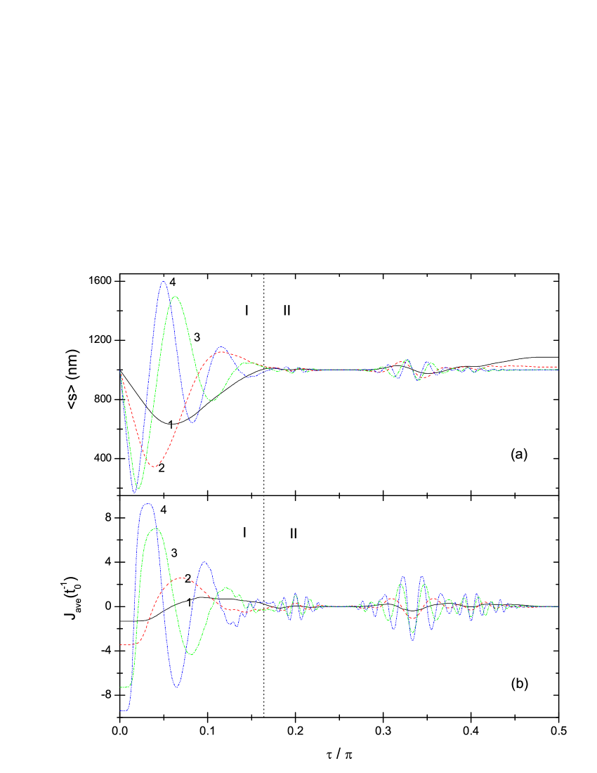
Figure 2: (Color online.) The time-dependence of the average position of the electron $\langle s\rangle$ and the average current $J_{ave}$ plotted in a quarter of a period. The curves ”1” to ”4” have $\Phi=1.25$, $3.25$, $6.85$, and $8.85$, respectively.

In order to have a general impression on the evolution, we define the time-dependent average position of the electrons

$$\langle s\rangle\equiv\int\rho(s,\tau)s\ ds$$ (14)

and define the time-dependent average current as

$$J_{ave}(\tau)\equiv\frac{1}{L}\int J(s,\tau)\ ds$$ (15)

When $\Phi$ is given at four values, $\langle s\rangle$ and $J_{ave}(\tau)$ against $\tau$ are shown in Fig.2. When $\tau=0$, obviously $\langle s\rangle=L/2$ (at the bottom) as shown in Fig.2a. However, the current is not zero initially ($J_{ave}(0)\neq 0$). This is shown in Fig.2b, where a larger $\Phi$ leads to a more negative $J_{ave}(0)$.

Let us define $E_{evol}=\langle\psi_{g}|H_{evol}|\psi_{g}\rangle$ which is the energy contained in $\psi_{g}$ after the transformation of the Hamiltonian. It was found that, when $\Phi$ increases from $1.25$ to $8.85$, $E_{evol}$ increases from $0.0152$ to $0.333meV$. Obviously, a larger $E_{evol}$ will lead to a stronger initial current which motivates the evolution afterward.

In Fig.2 the duration $[0,\pi/2]$ can be roughly divided into two, $[0,\pi/6]$ and $[\pi/6,\pi/2]$. In the former $\langle s\rangle$ goes toward the two ends alternately. Accordingly, $J_{ave}$ appears as negative and positive alternately. Obviously, this implies that the electron oscillates end-to-end repeatedly. When $\Phi$ is larger, the first minimum of $\langle s\rangle$ will shift down and left as shown in Fig.2a. It implies that, once the evolution begins, the electron will be closer to A in a shorter time. Furthermore, a larger $\Phi$ will cause more rounds of oscillation taking place in the duration $[0,\pi/6]$.

In the duration $[\pi/6,\pi/2]$, $\langle s\rangle$ remains to be close to $L/2$, and $|J_{ave}|$ becomes small. It implies that the probabilities of the electron staying at the left and right sides of the bottom are nearly equal, and both negative and positive currents might appear in the path simultaneously (this leads to a cancellation and thereby a smaller $|J_{ave}|$). The above two durations, for simplicity, are called duration of oscillation (DoS) and duration of cruise (DoC).

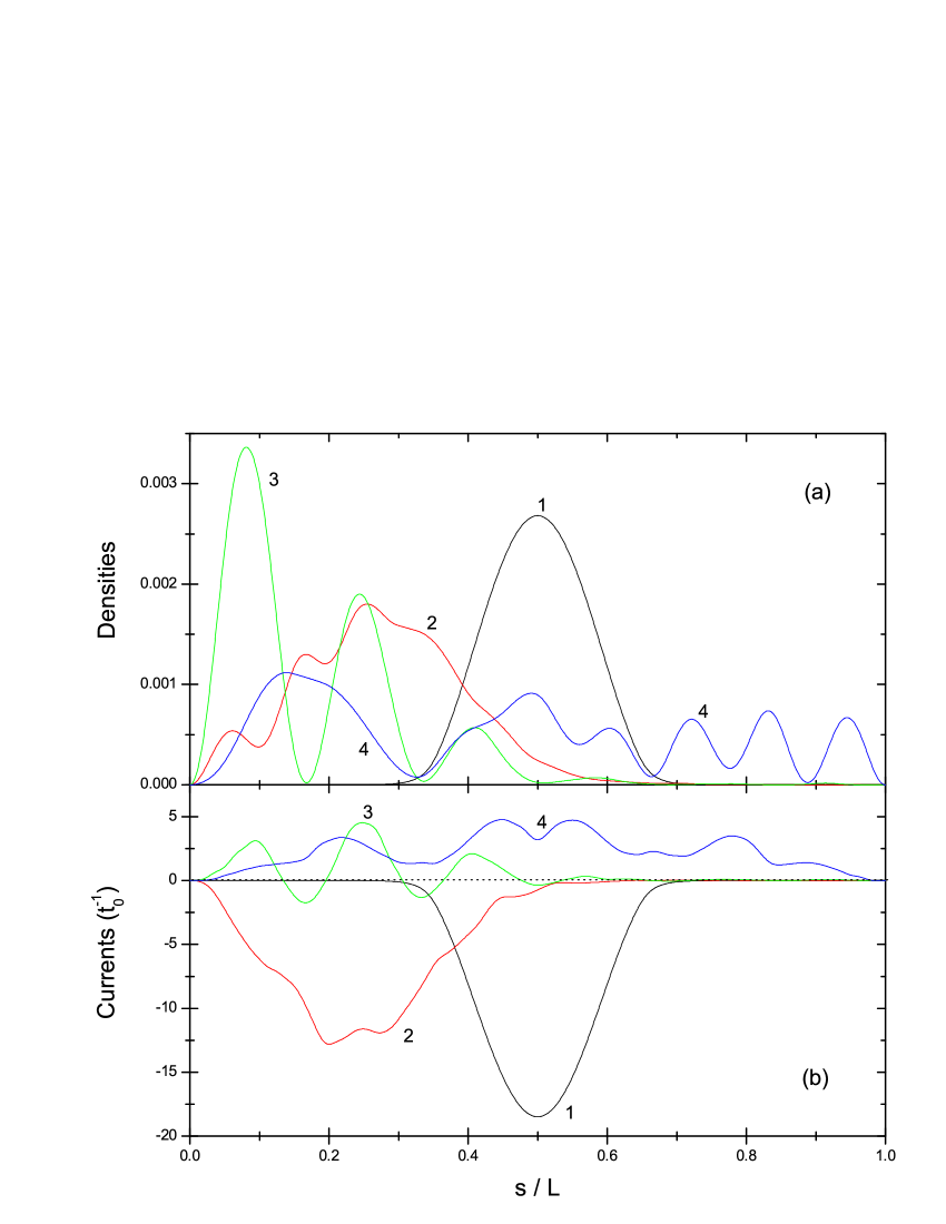
Figure 3: (Color online.) Spatial distribution of the densities $\rho(s,\tau)$ and currents $J(s,\tau)$ against $s$. The curves ”1” to ”4” have $\tau=0$, $\pi/48$, $\pi/24$, and $\pi/12$, respectively (these values are within the duration of oscillation DoS). The preset flux $\Phi=3.25$ (the same for Figs.3 to 6). The unit of current is $t_{o}^{-1}$, where $t_{o}\equiv 2m^{*}L^{2}/(\pi^{2}\hbar)$ is the unit of time used in this paper.

To study in detail the evolution in the DoS, the spatial distribution of $\rho(s,\tau)$ is plotted in Fig.3, where $\tau$ is given at four values in the early stage of evolution. When $\tau=0$, the curve ”1” of Fig.3a shows the initial localization, and ”1” of Fig.3b shows the strong negative initial current created via the sudden change of the Hamiltonian. Due to the negative current, the peak of $\rho$ shifts left rapidly as shown by ”2” of Fig.3a. Correspondingly, the distribution of $J$ shifts also left as shown by ”2” of Fig.3b. Afterward, the peak of $\rho$ keeps going left and will be close to A as shown by ”3” of Fig.3a. However, ”3” of Fig.3b is mainly positive. It implies that the direction of motion has already been reversed and the electron begins going toward the other end E. A little time later, the density is partially close to E as shown by ”4” of Fig.3a. Meanwhile, the current is positive throughout the path as shown by ”4” of Fig.3b. Accordingly, the distribution of $\rho$ as a whole is going right. Fig.3 shows only the first round of oscillation in the DoS when $\Phi=3.25$.

The maximal initial current $J(L/2,0)$ (e.g., the dip of ”1” of Fig.3b) was found to be nearly linearly proportional to $\Phi$ (with our parameters, $J(L/2,0)\approx-5.69\Phi/t_{o}$). Incidentally, if $\Phi<0$, the initial current would be positive and therefore the direction of motion would be reversed.

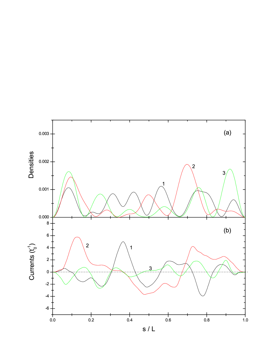
Figure 4: (Color online.) The same as Fig.3 but in the duration of cruise DoC $[\pi/6,\pi/2]$. The curves ”1” to ”3” have $\tau=0.285\pi$, $0.354\pi$, and $0.458\pi$, respectively.

In the DoC both $\rho$ and $J$, in general, are widely distributed along the path from A to E with numbers of peaks and dips as shown in Fig.4. In this duration the current may be positive (going right) somewhere and negative (going left) elsewhere. If $J=0$ and $\frac{\partial}{\partial s}J>0$ take place at $s=s_{o}$, there would be a source at $s_{o}$ from where the current flows out to both sides. Whereas if $J=0$ and $\frac{\partial}{\partial s}J<0$ at $s_{o}$, there would be a leak to where the currents flow in from both sides. Both sources and leaks are found in the path. The classical picture of motion of the electron in the DoC is not clear, it seems to be chaotic.

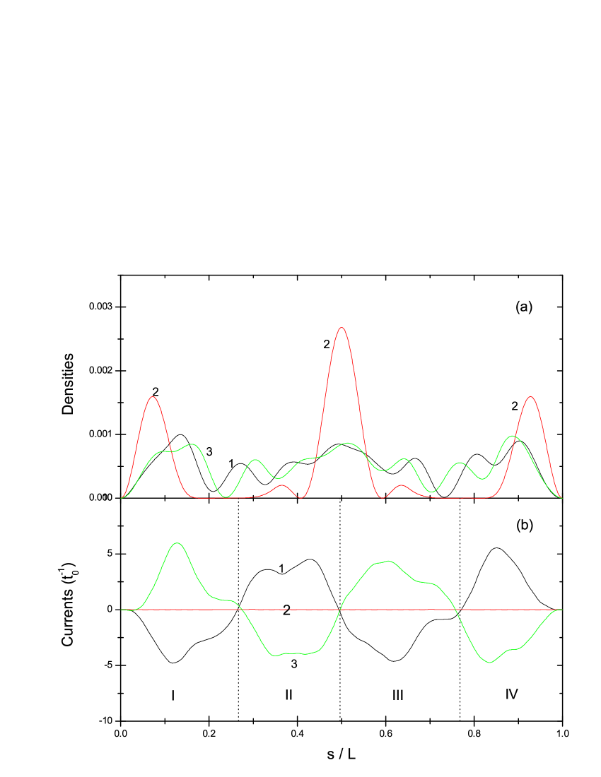
Figure 5: (Color online.) The same as Fig.3 but the curves ”1” to ”3” have $\tau=\pi/4-\pi/96$, $\pi/4$, and $\pi/4+\pi/96$, respectively.

However, in the DoC, there is a noticeable instant. When $\tau=\pi/4$, we have $\langle s\rangle=L/2$ and $J_{ave}=0$ disregarding how $\Phi$ is as shown in Fig.2. At this instant $\rho$ is no more widely distributed but concentrated close to the two ends and the bottom C as shown by ”2” of Fig.5a (where the peak at the bottom is much higher). When $\tau$ is a little earlier and later than $\pi/4$, $\rho$ and $J$ are shown, respectively, by ”1” and ”3” of Fig.5a and 5b. They together demonstrate how the density is concentrated into three peaks and spread out afterward. The abscissa of Fig.5b has been divided into four regions. The curve ”1” of Fig.5b is negative in region I. Thus the density is pushed left resulting in forming the peak of $\rho$ close to A. Besides, ”1” is positive in II but negative in III. Thus $\rho$ is pushed from both sides of C to the bottom resulting in forming the highest peak. Furthermore, the positive current in IV leads to the peak close to E. Exactly at the instant $\tau=\pi/4$, the current is zero as shown by ”2” of Fig.5b. It implies that the system is static instantaneously. Afterward, the current increases rapidly but in reverse direction as shown by ”3” of Fig.5b. This leads to the disappearance of the three peaks as shown by ”3” of Fig.5a. The existence of instants wherein the system is instantaneously static is not at all surprising, this might happen in various types of oscillation (say, in classical pendulum).

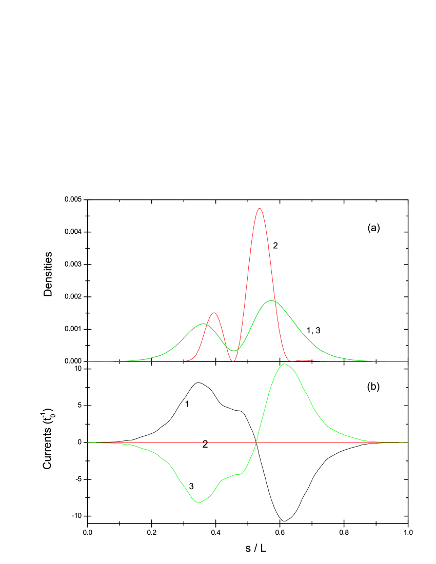
Figure 6: (Color online.) The same as Fig.3 but the curves ”1” to ”3” have $\tau=\pi/2-\pi/96$, $\pi/2$, and $\pi/2+\pi/96$, respectively.

When $\tau$ is close to $\pi/2$, the density is once again concentrated in the bottom as shown by ”2” of Fig.6a, where the main peak is very sharp and high. At the same time, the associated current (”2” of Fig.6b) is exactly zero (this is obvious from Eq.(12)). Thus the system becomes once again static instantaneously. ”1” and ”3” of 6a describe the densities a little earlier and later, respectively, than $\pi/2$. They overlap exactly due to the symmetry given in Eq.(10). ”1” and ”3” of Fig.6b are exactly opposite to each other due to Eq.(12). In fact, they cause a rapid gathering and, successively, a rapid extension of $\rho$. In particular, the exact symmetry appearing in Fig.6b implies that the evolution has arrives at a turning point. Afterward, the evolution will proceed exactly reversely as demonstrated by Eqs.(10) and (12). For examples, the density will be re-gathered into three peaks exactly as ”2” of Fig.5a when $\tau=3\pi/4$, and will re-visit A exactly as ”3” of 3a when $\tau=\pi-\pi/24$, etc. When $\tau=\pi$, $\rho$ is exactly as ”1” of 3a, while $J$ is exactly opposite to ”1” of Fig.3b. Thus, instead of going left, the peak of $\rho$ at the bottom goes right at $\tau=\pi$ due to the positive $J$.

It is noted that from Eqs.(10) and (11), we have

$$\rho(L-s,\tau)=\rho(s,\pi+\tau)$$ (16)

From (12) and (13), we have

$$J(L-s,\tau)=-J(s,\pi+\tau)$$ (17)

In the duration $[\pi,2\pi]$, Eqs.(16) and (17) together imply that the evolution is just a repeat of that from $0$ to $\pi$, but with an interchange $s\longleftrightarrow L-s$ (namely, an interchange of the A and E ends). Thus, the evolution in the whole period $2\pi$ is completely clear, and it goes on again and again periodically.

Now let us compare the current in the U-oscillator with the famous Aharonov-Bohm (A-B) persistent current of an electron on a ring. The maximal A-B current of the ground state is $J_{A-B}=\hbar/(4\pi m^{*}R^{2})$. Thus, $t_{o}^{-1}=2\pi(L-2l)^{2}/L^{2}\ J_{A-B}$. For our parameters, we found that $J(L/2,0)=-12.87\Phi J_{A-B}$. Thus, giant current can be obtained if $\Phi$ is sufficiently strong (say, if $\Phi\approx 10$, $J(L/2,0)$ is two orders stronger than the A-B current).

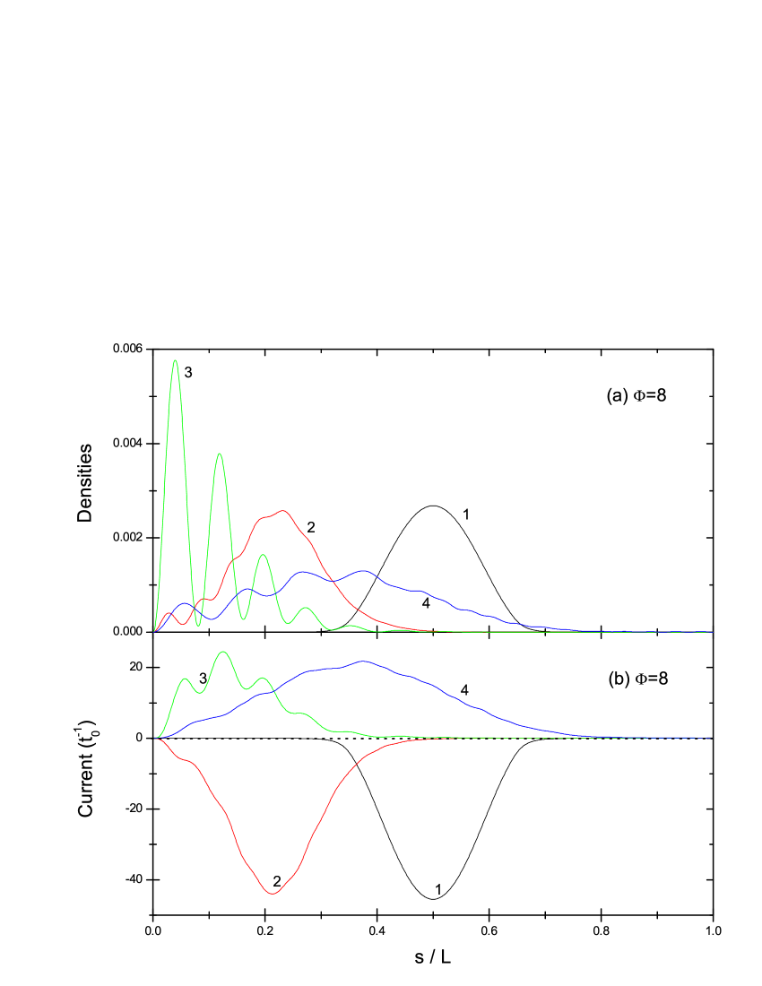
Figure 7: (Color online.) $\rho(s,\tau)$ and $J(s,\tau)$ with $\Phi=8$. The curves ”1” to ”4” have $\tau=0$, $\pi/96$, $\pi/48$, and $\pi/32$, respectively.

Since $t_{o}$ is proportional to $m^{*}L^{2}$, a longer path and/or a heavier effective mass will lead to a longer period. The preset $\Phi$ as a motivity is crucial to the oscillator. Its effect has been shown in Fig.2 and is further shown in Fig.7 with $\Phi=8$ (to be compared with Fig.3 with $\Phi=3.25$). Comparing the distributions of ”3” of Fig.7a and Fig.3a, the former is closer to A and occurs much earlier (the electron rushes to A more rapidly). While $\Phi$ is a very sensitive factor, the parameters of the preset potential is less sensitive to the evolution.

Figure 8: The time-dependence of $\langle s\rangle$ in a whole period. $\Phi=3.25$ (a) and $8$ (b).

In summary, a U-oscillator has been proposed and studied. The motion of electron in the device is strictly periodic and adjustable. The following points are reminded

(i) When $t_{o}$ is used as the unit of time, the period is $2\pi$. The evolution in the second quarter of a period is the time-reversal of that of the first quarter, and the evolution in the second half is the same as the first half but with the interchange $s\longleftrightarrow L-s$, namely, a spatial reflection against $L/2$.

(ii) Each quarter can be divided into two durations, namely, DoS and DoC. The classical picture in the former is clear (a few rounds of oscillation appear), but not clear in the latter. When $\Phi$ is larger, more rounds of oscillation will appear in the DoS.

(iii) Let the time associated with the lowest minimum of Fig.2a be $\tau_{end}$. Then, in the first half period, the electron is very close to A twice at $\tau_{end}$ and $\pi-\tau_{end}$, respectively. Whereas in the second half period, the electron is very close to E also twice at $\pi+\tau_{end}$ and $2\pi-\tau_{end}$, respectively. Such a close contact of the electron with the two ends in a whole period is shown in Fig.8, where the appearance of rounds of oscillation in the DoS is also clear. On the contrary with classical pendulum, it is clear from Fig.8 that is explicitly the end-to-end oscillation occurs only if $\tau$ is close to $I\pi$ ($I$ is a positive integer).

(iv) Each time when $\tau=I\pi/4$ , the system is instantaneously static, namely, $J(s,I\pi/4)=0$ for all $s$. Meanwhile, the density would be mostly concentrated in the neighborhood of C, namely, the bottom of the U-pipe.

(v) The introduction and the sudden removal of $\Phi$ is a crucial point. This leads to the sudden creation of the initial current, which motivates the evolution afterward. In particular, when $\Phi$ is sufficiently large, giant periodic current (two or more orders stronger than the A-B current) can be obtained.

The device might work as a quantum pendulum. It can be generalized to include a group of localized electrons initially. This case deserves to be further studied. The idea proposed in this paper might be useful in micro technology.

- (1) A. Lorke and R. J. Luyken, Physica B 256, 424 (1998)
- (2) A. Lorke, R. J. Luyken, A.O. Govorov, J.P. Kotthaus, J.M. Garcia, and P.M. Petroff, Phys. Rev. Lett. 84, 2223 (2000)
- (3) H. Pettersson, R. J. Warburton, A. Lorke, K. Karrai, J. P. Kotthaus, J. M. Garcia, and P. M. Petroff, Physica E 6, 510 (2000)
- (4) U. F. Keyser, C. Fühner, S. Borck, R. J. Haug, M. Bichler, G. Abstreiter, and W. Wegscheider, Phys. Rev. Lett. 90, 196601 (2003)
- (5) D. Mailly, C. Chapelier, and A. Benoit, Phys. Rev. Lett. 70, 2020 (1993)
- (6) A. Fuhrer, S. Lüscher, T. Ihn, T. Heinzel, K. Ensslin, W. Wegscheider, and M. Bichler, Nature (London) 413, 822 (2001)
- (7) A. E. Hansen, A. Kristensen, S. Pedersen, C. B. Sorensen, and P. E. Lindelof, Physica E 12, 770 (2002)
- (8) S. Viefers, P. Koskinen, P. Singha Deo, and M. Manninen, Physica E 21, 1 (2004)
- (9) Y. Z. He and C. G. Bao, arXiv:0805.1081v1 [cond-mat.other], 8 May 2008