MARKET MILL DEPENDENCE PATTERN IN THE STOCK MARKET: MULTISCALE CONDITIONAL DYNAMICS

Sergey Zaitsev^(a), Alexander Zaitsev^(a),
Andrei Leonidov^(b,a,c),, Vladimir Trainin^(a),

(a) Letra Group, LLC, Boston, Massachusetts, USA

(b) Theory Department, P.N. Lebedev Physics Institute, Moscow, Russia

(c) Institute of Theoretical and Experimental Physics, Moscow, Russia

Abstract

Market Mill is a complex dependence pattern leading to nonlinear correlations and predictability in intraday dynamics of stock prices. The present paper puts together previous efforts to build a dynamical model reflecting the market mill asymmetries. We show that certain properties of the conditional dynamics at a single time scale such as a characteristic shape of an asymmetry generating component of the conditional probability distribution result in the ”elementary” market mill pattern. This asymmetry generating component matches the empirical distribution obtained from the market data. We discuss these properties as a mixture of trend-preserving and contrarian strategies used by market agents. Three basic types of asymmetry patterns characterizing individual stocks are outlined. Multiple time scale considerations make the resulting ”composite” mill similar to the empirical market mill patterns. Multiscale model also reflects a multi-agent nature of the market.

1 Introduction

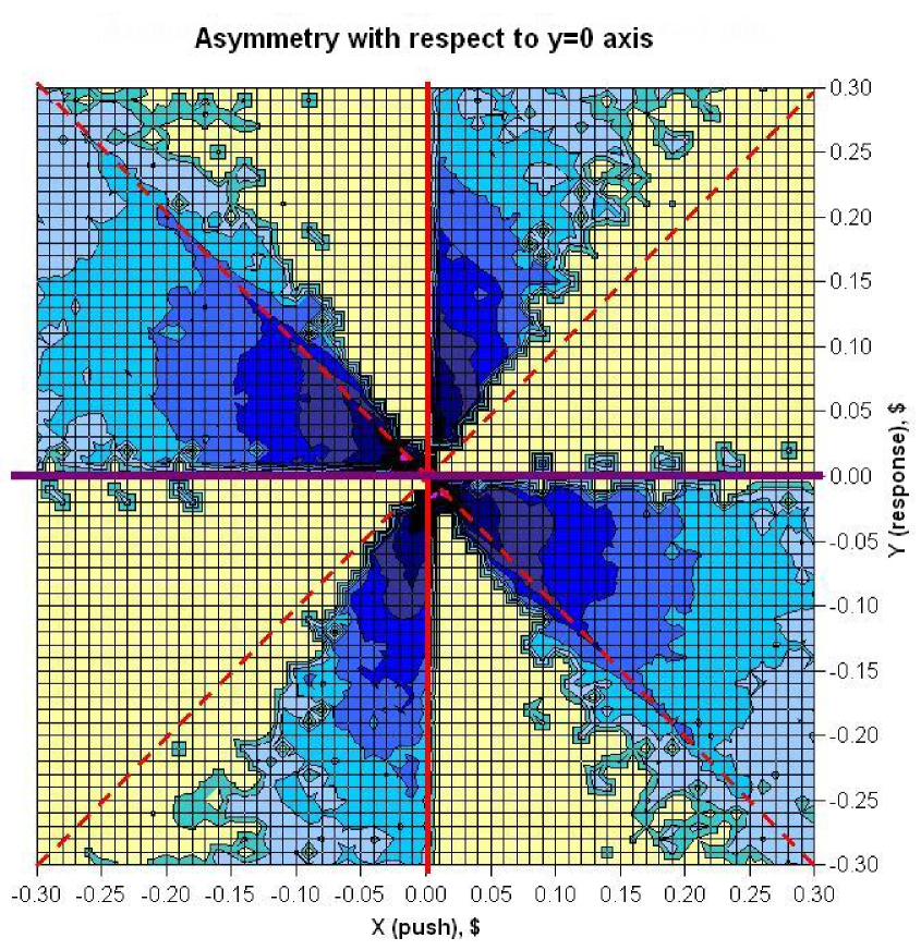
Figure 1: The market mill pattern, [5].

The present paper continues a series of papers studying the complex dependence patterns in high frequency stock price dynamics [1, 2, 3, 4, 5]. The most important of them, the market mill asymmetries [2, 3, 4, 5], correspond to specific probabilistic interrelations between consequent price increments. The term ”market mill” refers to a mill-like asymmetric four-blade dependence pattern [2], see Fig. 1. The main emphasis of [2, 3, 4] was on systematic phenomenological description of the market mill asymmetries and other related properties of high frequency stock price dynamics.

In [5] a causal conditional dynamics model leading to the market mill asymmetries and nonlinear dependence of expectation value of a future price increment y (”response”) on the value of a realized price increment x (”push”) was suggested. The model described probabilistic relation between the push $x$ and the response $y$ in terms of the three - component conditional distribution ${\cal P}(y|x)$. The distribution ${\cal P}(y|x)$ was described as an $x$-dependent additive superposition of the symmetric contribution ${\cal P}^{0}(y|x)$ and the asymmetry-generating components ${\cal P}^{+}(y|x)$ and ${\cal P}^{-}(y|x)$ characterized by a bias towards trend-preserving and contrarian strategies correspondingly. The model of [5] referred to a single time scale.

It is however well known that a description of certain features of stock price dynamics requires accounting for multiple time scales, at the level of both price increments (returns) [6, 7, 8, 9, 10, 11, 12, 13] and microscopic long-memory properties of order flow and trades [14, 15, 16]. In particular, the presence of several distinct time scales in volatility dynamics was explicitly demonstrated in [9]. In [2] the empirical market mill patterns were shown to exist at different time scales ranging from minutes to hours.

In the present paper we incorporate the idea of multiple time scales into the market mill model. First we introduce an elementary market mill mechanism at a fixed time scale. We describe an easier way of specifying the elementary market mill by reformulating the model of [5] in such a way that $y$ is a sum of noise and non-random asymmetry generating components. Introducing specific features of the non-random component based on empirical data we come up with the market mill pattern. Then we build a multiscale composite mill as a weighted superposition of elementary asymmetry-generating mechanisms operating at different timescales.

The outline of the paper is as follows.

We start with a description of generic features of the market mill asymmetries in paragraph 2.1. Particular emphasis is put onto formulating a version stock price dynamics with an additive superposition of noise and asymmetry-generating mechanisms. In paragraph 2.2 we describe the conditional distribution allowing to reproduce all observed market mill asymmetries. The properties of explicit dynamical model giving rise to a single time scale elementary market mill asymmetries are discussed in paragraph 2.3. The composite multiscale dynamics allowing to reproduce all the properties of the market mill asymmetries is described in paragraph 2.4. The section 3 contains a discussion of the origin of the market mill asymmetries in terms of three basic strategies, market mill, trend-following and contrarian, used by market participants. We demonstrate that appropriately weighted superpositions of these basic strategies allows to describe various two-dimensional asymmetry patterns characterizing individual stocks. We formulate our conclusions in section 4.

2 Conditional dynamics

2.1 Qualitative features

At the fundamental level the ultimate goal of studying the dependence patterns in price dynamics is to describe the observed dependence patterns between price increments $x=p(t_{1}+\Delta T)-p(t_{1})$ and $y=p(t_{2}+\Delta T)-p(t_{2})$, where $t_{2}\geq t_{1}+\Delta T$, in terms of explicit strategies used by market participants. These strategies are realized through systematic reaction of market participants to the information about the sign and magnitude of the increment $x$ leading to some predictability of the increment $y$. A strategy is thus fully described by probabilistic properties of $y$ at given $x$ i.e. by a conditional distribution ${\cal P}(y|\,x)$. An existence of dependence patterns relating the push $x$ and the response $y$ is then reflected in systematic non-random features of ${\cal P}(y|\,x)$ which induce, in turn, dependence patterns of the full bivariate distribution ${\cal P}(x,y)$ such as the market mill ones.

Let us describe the most important properties of ${\cal P}(y|\,x)$ following from an analysis of empirical data. To this aim let us introduce an additive decomposition of the response $y$ into noise $y_{\rm rand}$ and systematic $y_{\rm mill}$ contributions:

$$y(x)\,=\,y_{\rm rand}(x)+y_{\rm mill}(x)\,,$$ (1)

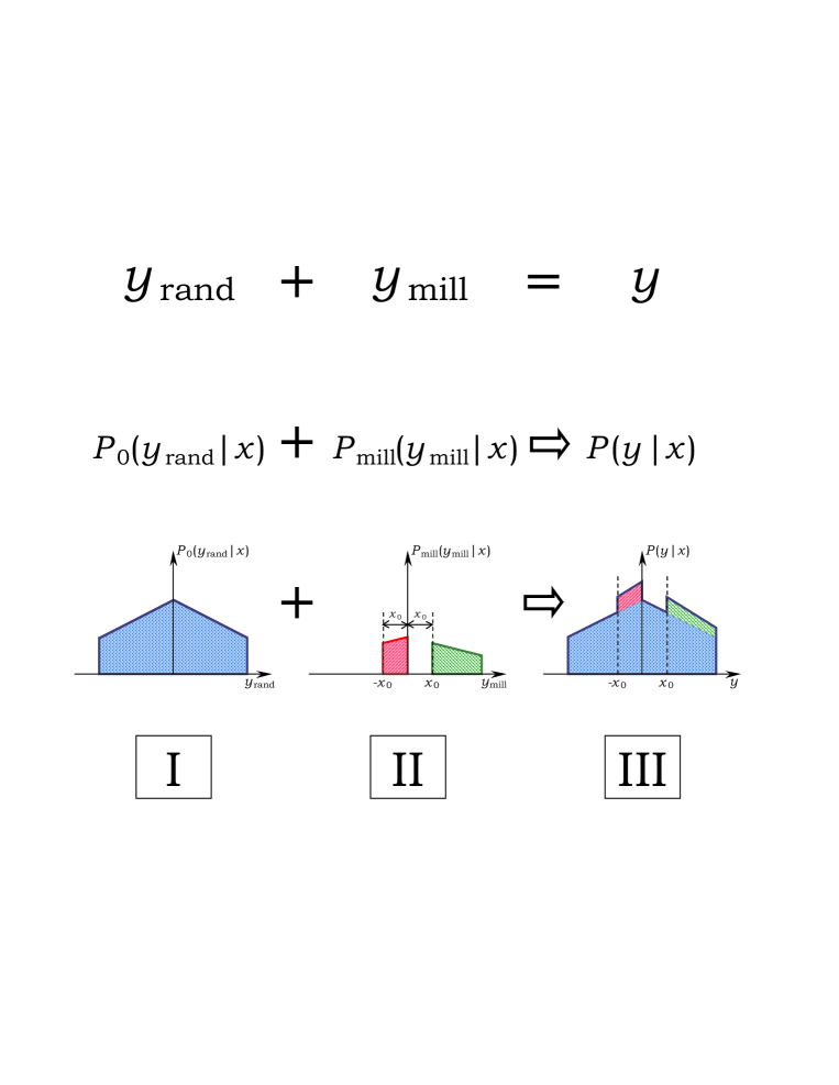
Figure 2: Sketch of the asymmetry-generating conditional dynamics

where the random component $y_{\rm rand}(x)$ is described by a distribution ${\cal P}_{0}(y_{\rm rand}|\,x)$ and the systematic component $y_{\rm mill}$ is described by a distribution ${\cal P}_{\rm mill}(y_{\rm mill}|\,x)$. The probability distribution for $y(x)$ is, naturally, ${\cal P}(y|\,x)$. A graphic illustration of the decomposition (1) and qualitative features of the corresponding probability distributions ${\cal P}_{0}(y_{\rm rand}|\,x)$, ${\cal P}_{\rm mill}(y_{\rm mill}|\,x)$ and ${\cal P}(y|\,x)$ is given, for the positive push $x$, in Fig. 2 in columns I, II and III respectively. Let us note that the above additive decomposition is very natural from the point of view of an agent-based description where the orders originating from different strategies are added in the time interval under consideration at each evolution step.

The distribution ${\cal P}_{0}(y_{\rm rand}|\,x)$ is a symmetric function of its argument, ${\cal P}_{0}(y_{\rm rand}|\,x)={\cal P}_{0}(-y_{\rm rand}|\,x)$, see column I in Fig. 2, and describes the main contribution to the conditional dynamics. Market data shows [3, 5] that the relative weight of the symmetric contribution is dominant with respect to the asymmetric one.

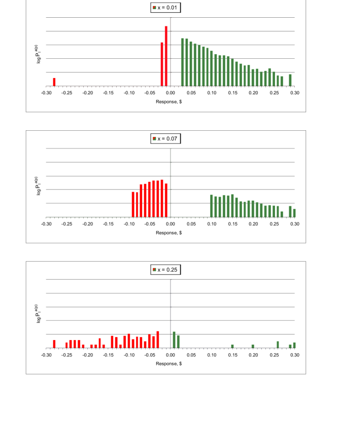
Figure 3: The observed mill distribution ${\cal P}_{\rm mill}(y_{\rm mill}|\,x)$ at different $x$ [2].

On top of the dominating random dynamics described by ${\cal P}_{0}(y_{\rm rand}|\,x)$ there exists a systematic asymmetry-generating dynamics described by ${\cal P}_{\rm mill}(y_{\rm mill}|\,x)$ illustrated in column II of Fig. 2 for $x=x_{0}>0$. Its message can be formulated in a simple statement. If the push $x$ is followed by the response $y$ that does not exceed $x$ by magnitude, it is slightly more probable that the response is contrarian, ${\rm sign}(y)=-{\rm sign}(x)$. For responses with the magnitude exceeding that of the push it is, on contrary, more probable that the response is trend-following, ${\rm sign}(y)={\rm sign}(x)$. For example, for positive pushes $x>0$ there is a small bias towards responses of two sorts: those in the interval $y\in[-x,0]$ and those in the interval $y>x$. Let us note that this particular property of ${\cal P}_{\rm mill}(y_{\rm mill}|\,x)$ also goes along with the empirically observed features, see Fig. 3.

The above-described coexistence of dominating symmetric and subdominant asymmetric responses leads to the total distribution with the shape sketched in column III in Fig. 2. Technically the conditional distribution ${\cal P}(y|\,x)$ is given by an appropriate convolution of the distributions of the random and systematic components

$${\cal P}(y|\,x)=\int dy_{\rm rand}dy_{\rm mill}\,\delta(y-y_{\rm rand}-y_{\rm mill})\,{\cal P}_{0}(y_{\rm rand}|\,x)\,{\cal P}_{\rm mill}(y_{\rm mill}|\,x)$$ (2)

With the specified probabilistic model for the conditional distribution ${\cal P}(y|\,x)$ the last step is to establish its relation to the full bivariate distribution ${\cal P}(x,y)$ and its asymmetry patterns. Let us remind that the specific dependence patterns of major interest to us, the market mill asymmetries [2, 3, 4], refer to specific asymmetries of the bivariate distribution ${\cal P}(x,y)$ with respect to the axes $x=0$, $y=x$, $y=0$ and $y=-x$.

First, one reconstructs the bivariate distribution ${\cal P}(x,y)$ from conditional dynamics described by ${\cal P}(y|\,x)$. This reconstruction is based on the relation ${\cal P}(x,y)={\cal P}(y|\,x){\cal P}(x)$, where ${\cal P}(x)$ is a corresponding marginal distribution.

The market mill asymmetry patterns are described in terms of corresponding nontrivial asymmetric components ${\cal P}^{a}(x,y)$ of the distribution ${\cal P}(x,y)$. For example, for the asymmetry with respect to the axis $x=0$ this asymmetric component reads

$${\cal P}^{a}\,=\,\frac{1}{2}\left({\cal P}(x,y)-{\cal P}(x,-y)\right)$$ (3)

The corresponding market mill dependence pattern refers [2] to the specific shape of ${\cal P}_{\rm mill}(x,y)\equiv{\cal P}^{a}(x,y)\cdot\Theta\left[{\cal P}^{a}(x,y)\right]$, where $\Theta$ is the Heaviside step function. The asymmetric components ${\cal P}^{a}(x,y)$ are also responsible for nontrivial conditional dependencies between $y$ and $x$. For example, again in the case of the asymmetry with respect to the axis $x=0$, the mean conditional response $\langle y\rangle_{x}$ ,

$$\langle y\rangle_{x}\,=\,\int dy\,y\,\frac{{\cal P}^{a}(x,y)}{{\cal P}(x)}\,,$$ (4)

has a specific $z$-shaped dependence on $x$ [2].

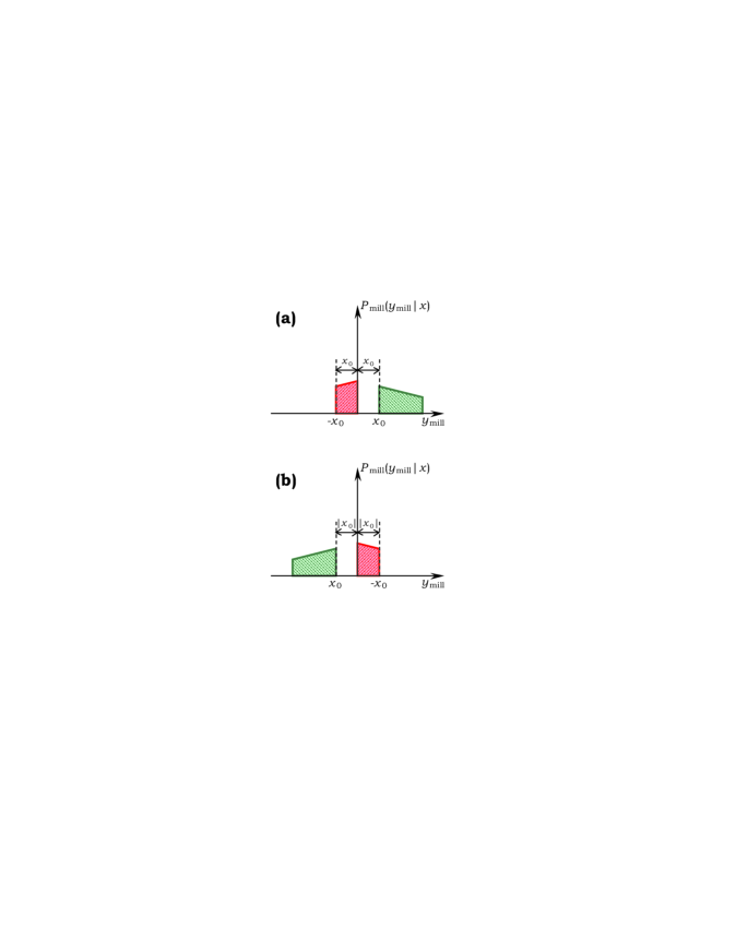
Figure 4: Asymmetry generating component of the conditional probability distribution ${\cal P}_{\rm mill}(y_{\rm mill}|\,x)$; (a) $x_{0}>0$; (b) $x_{0}<0$.

The required identification of noise and asymmetry-generating components of ${\cal P}(y|\,x)$ is achieved [2] by extracting, in complete analogy with the above-described procedure for the bivariate distribution ${\cal P}(x,y)$, the symmetric and mill components of ${\cal P}(y|\,x)$. One could say that ${\cal P}_{\rm mill}(y_{\rm mill}|\,x)$ contains ”irreducible” information on the asymmetry-generating dynamics. The experimentally measured mill component [2] is shown in Fig. 3. The explicit version of conditional dynamics described in the next paragraph is based on stylized features of ${\cal P}_{\rm mill}(y_{\rm mill}|\,x)$ following from the analysis of Fig. 3 and illustrated in Fig. 4. Let us stress once again that from the shape of the mill component shown in Figs. 3,4 it is clear that the systematic asymmetry-generating contribution $y_{\rm mill}(x)$ originates from both trend-preserving and contrarian order placement.

2.2 Quantitative formulation

Let us now turn to a step-by-step description of the conditional dynamics in question.

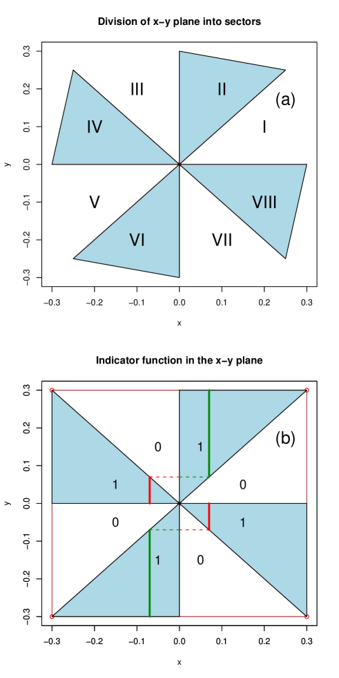
Figure 5: Sectors in $x-y$ plane [2].

A compact description of the conditional distributions shown in Figs. 2-4 can be given by dividing the $x-y$ plane into eight sectors [2] shown in Fig. 5 and introducing an indicator function $f_{\rm mill}(x,y)$ equal to $1$ in the even sectors and equal to $0$ in the odd ones, see Fig. 5(a). Then

$${\cal P}_{\rm mill}(y_{\rm mill}|\,x)\,=\,f_{\rm mill}(x,y_{\rm mill})\,{\cal P}_{0}(y_{\rm mill}|\,x)$$ (5)

where ${\cal P}_{0}(y|\,x)$ is a symmetric distribution of the response $y$ at some fixed push $x$. The indicator function $f_{\rm mill}(x,y)$ cuts from ${\cal P}_{0}(y|\,x)$ the pieces having support on the corresponding segments of the $y$ axis. These cuts and the corresponding support intervals in the $y$ axis are shown, for $x=\pm\$\,0.07$, in Fig. 5(b). The lines in the shaded areas correspond to the segments of the $y$ axis carrying nonzero contribution to ${\cal P}(y|\,x)$ in Fig. 3.

We see that the structure of systematic response $y_{\rm mill}$ depends, in an essential way, on the sign of the push $x$.

Let us first assume that the push $x$ is positive, $x>0$. The corresponding response $y_{\rm mill}$ could be positive or negative. For $y_{\rm mill}>0$ its value lies in the interval $y_{\rm mill}>x$ with the probabilistic weight determined by the part of distribution in Fig. 4 (a) marked with green. For $y_{\rm mill}<0$ its value lies in the interval $y_{\rm mill}\in[-x,0)$ with the probabilistic weight determined by the part of distribution in Fig. 4(a) marked with red.

In terms of systematic strategies of market agents this corresponds to a push-dependent mixture of trend-preserving and contrarian strategies. Indeed, the part of distribution in Fig. 4(a) marked with green corresponds to trend-preserving order placement favoring the price growth while that marked with red is contrarian and corresponds to that favoring its decline.

If the push is negative, $x<0$, the response could again be negative or positive. For $y_{\rm mill}<0$ its value lies in the interval $y_{\rm mill}<x$ with the probabilistic weight determined by the part of distribution in Fig. 4 (b) marked with green. For $y_{\rm mill}>0$ its value lies in the interval $y_{\rm mill}\in(0,-x]$ with the probabilistic weight determined by the part of distribution in Fig. 4(b) marked with red. Here again we see a push-dependent mixture of trend-preserving (green) and contrarian (red) strategies.

The technical message of Figs. 2-5 is that a procedure of constructing
${\cal P}_{\rm mill}(y_{\rm mill}|\,x)$ consists in cutting appropriate pieces from the symmetric distribution ${\cal P}_{0}(y|\,x)$.

In our simulations described below we shall assume, for simplicity, that ${\cal P}_{0}(y_{\rm mill}|\,x)$ does not depend on $x$  and use a Laplace distribution

$${\cal P}_{0}(y)=\frac{1}{2\sigma_{\Delta T}}\exp\left\{-\frac{|\,y|}{\sigma_{\Delta T}}\right\}$$ (6)

that gives a reasonably good description of the bulk of the distribution of price increments at small intraday timescales.

Then for small $|\,x|<\log 2\cdot\sigma_{\rm\Delta T}$ a dominating strategy is the trend-preserving one while for large $|\,x|>\log 2\cdot\sigma_{\rm\Delta T}$ this is a contrarian one.

In what follows the asymmetry-generating distributions (5) will be used for explicitly constructing a series of price increments combining the noise $y_{\rm rand}$ and asymmetric $y_{\rm mill}$ contributions. In this construction a decision of using the systematic strategy is also randomized. In our simulations we first generate the noise increment price series using the distribution (6). Then we move along this price series and, at each step, decide whether a nontrivial asymmetry-generating contribution will be added to the noise increment in one of the following time intervals. Thus, in addition to knowing how to generate the asymmetry-generating component as described by (5), we have to decide whether, for a given realized price increment $x$, the asymmetric contribution is generated and define an interval in which the systematic price increment will be added. It is convenient to first specify a target interval and then either generate a nontrivial contribution to the increment in this interval or leave the interval’s increment untouched.

Randomization of an appearance of the asymmetry-generating component is realized by assuming that at each step the asymmetry-generating contribution is either switched on with a push-dependent probability $\nu(x)$ or switched off with a probability $1-\nu(x)$. If it is switched off a zero contribution $y_{\rm mill}=0$ is generated.

2.3 Single-scale conditional dynamics. Elementary mill

Let us now describe an explicit numerical realization of the dynamical model described in the previous paragraph. This model is an additive superposition of a trivial memoryless dynamics generating uncorrelated price increments sampled from the symmetric distribution ${\cal P}_{0}(y_{\rm rand})$ and the above-described nontrivial conditional dynamics generating asymmetric response $y_{\rm mill}$ for a given push $x$ in the interval separated from that corresponding to the push by a randomly chosen number of intervals $l$. The single-scale conditional dynamics corresponding to the elementary mill is then fully specified by selecting a distribution ${\cal P}(l|L)$ in the number $l-1$ of time intervals separating those corresponding to the push $x$ and the response $y_{\rm mill}$ where the parameter $L$ controls a shape of this distribution. In what follows we shall use ${\cal P}(l|L)\propto\exp(-l/L)$ with $L=3$. More precisely, when reaching a time interval with the realized price increment $x$ in it:

1. If $x\neq 0$ in a fraction of $\nu_{0}=0.12$ cases an additional price increment $y_{\rm mill}$ sampled from ${\cal P}(y_{\rm mill}|\,x)$ is added to the preexisting increment in the interval at some distance $l\,\Delta T$ from the interval with the realized increment $x$ where $l$ is sampled from ${\cal P}(l|L)$.

2. If $x=0$ no action is taken.

3. The basic symmetric distribution ${\cal P}_{0}(y)$ is a Laplace one (6) and the width of the ”elementary” distribution $\sigma=\$\,0.02$ corresponds to the observable standard deviation of price increments for $\Delta T_{0}=1\,{\rm min.}$.

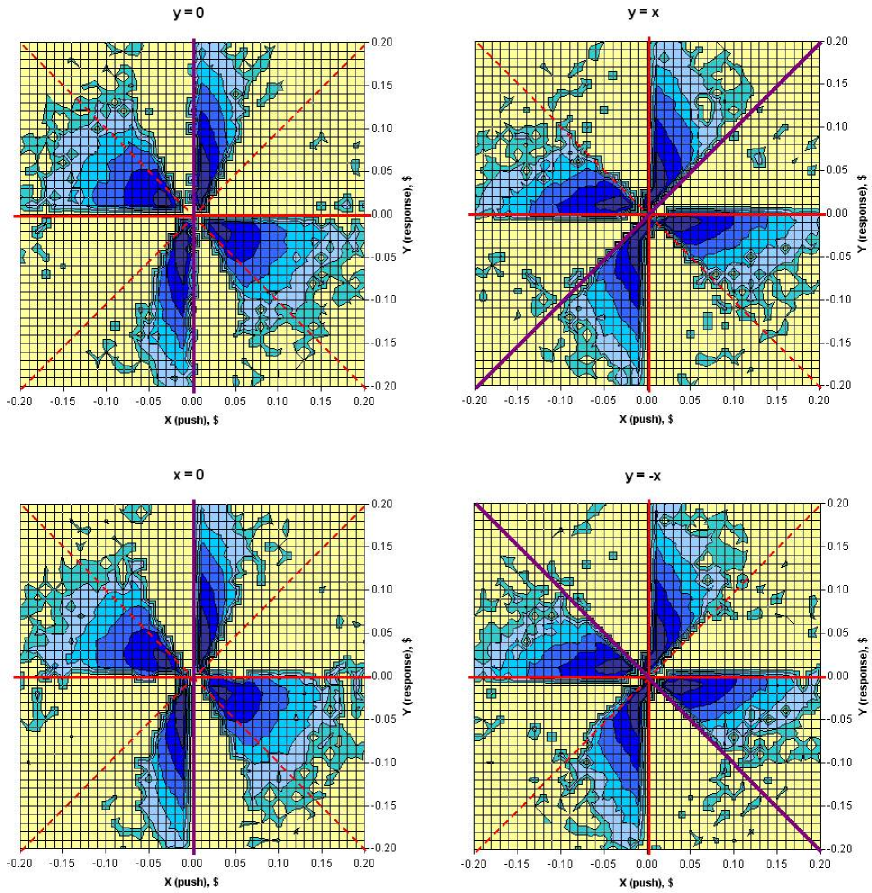
Figure 6: Model market mill patterns with respect to the axes $y=0$, $y=x$, $y=0$, $y=-x$, elementary mill, $\Delta T=1\,{\rm min}$.

The resulting four mills corresponding to the asymmetries with respect to the axes $x=0$, $x=y$, $y=0$ and $y=-x$ are shown in Fig. 6. We see that the the model gives a very good description of all the four market mill asymmetries.

From the analysis of market data we know that the market mill patterns are observed at different intraday time scales. Because of the response delay built in into the model one expects that the 1-minute elementary mill will propagate some millness to asymmetries measured at larger time intervals. To analyze this issue, let us again turn to the division of the $x-y$ plane into eight sectors [2], see Fig. 5(a), and introduce as a quantitative measure of ”millness” the quantity $\rho_{\rm mill}$ which is a relative difference between the density of even and odd sectors in the domain $\{x,y\}\in[-\delta p^{*},\delta p^{*}]$:

$$\rho_{\rm mill}\,=\,\frac{(n_{8}-n_{1})+(n_{2}-n_{7})+(n_{6}-n_{3})+(n_{4}-n_{5})}{n_{\rm tot}}$$ (7)

where $\{n_{i}\}$ are numbers of points generated within an $i$-th sector of this square. In our analysis we used $\delta p^{*}=\,\$\,0.3$.

The mean millness $\langle\rho_{\rm mill}\rangle$ and its standard deviation $\sigma(\rho_{\rm mill})$ computed for the market data for 2000 stocks traded at NYSE and NASDAQ stock exchanges in 2004-2005 for a set of time intervals $\Delta T=1,3,6\,{\rm min}$ are shown in the first two rows of Table 1. In this computation the total set of stocks was randomly divided into 20 groups containing 100 stocks each. In this way we obtained 20 values for $\rho_{\rm mill}$ within each group. Their mean and standard deviation are the numbers shown in Table 1.

In our theoretical simulations we created, for each case considered, 2000 time series of the same length as in the above-described market data which we also divide into 20 subsets containing 100 time series each. The corresponding mean values and standard deviations characterizing theoretical millness are computed from 20 values characterizing these 20 subsets.

In the third and fourth row of Table 1 we show the mean millness and its standard deviation for the elementary market mill model. We see that, at variance with experimental observations, the original millness generated by the elementary mill at the scale of $\Delta T=1\,{\rm min}$ gradually weakens with growing time interval $\Delta T$.

Table 1.

Source	Quantity	$\Delta T=1{\rm min}$	$\Delta T=3{\rm min}$	$\Delta T=6{\rm min}$
Market data	$\langle\rho_{\rm mill}\rangle$	1.52	2.32	2.32
Market data	$\sigma\left(\rho_{\rm mill}\right)$	0.07	0.08	0.10
Elementary mill	$\langle\rho_{\rm mill}\rangle$	1.85	0.94	0.39
Elementary mill	$\sigma\left(\rho_{\rm mill}\right)$	0.02	0.02	0.04
Composite mill	$\langle\rho_{\rm mill}\rangle$	0.87	1.71	1.71
Composite mill	$\sigma\left(\rho_{\rm mill}\right)$	0.01	0.04	0.04

Table 1. Values of mean millness and its standard deviation (both in percent) for market data, elementary and composite mills.

2.4 Multiscale conditional dynamics. Composite mill

The analysis in the previous section has shown that the observable initial growth and consequent constancy of millness $\rho_{mill}(\Delta T)$ can not be achieved by considering a single elementary mill operating at some ”starting” scale $\Delta T_{0}$. A natural generalization of this construction is achieved by augmenting conditional dynamics corresponding to the elementary mill by adding, with some weights, conditional dynamics mechanisms operating at larger time scales. More explicitly, let us consider a sequence of time scales $\{\Delta T_{i}=i\,\Delta T_{0}\}$. Then at some given moment $t$ there is a probability $\nu_{1}$ of switching on an asymmetric conditional dynamics at the scale $\Delta T_{0}$, a probability $\nu_{2}$ of switching on an asymmetric conditional dynamics at the scale $2\cdot\Delta T_{0}$, etc.

Let us consider as an example a superposition of two mills operating at time scales $\Delta T_{0}$ and $2\cdot\Delta T_{0}$.

For the first dynamics the push at time $t$ is a price increment $\delta P([t-\Delta T_{0},t])$ and the response is generated in the interval $[t+l_{1}\Delta T_{0},t+(l_{1}+1)\Delta T_{0}]$ where $l_{1}$ is sampled from ${\cal P}(l|L)$ and the standard deviation of the response is $\sigma_{\Delta T_{0}}$.

For the second dynamics the push at time $t$ is a price increment $\delta P([t-2*\Delta T_{0},t])$ and the response is generated in the interval $[t+l_{2}\Delta T_{0},t+(l_{2}+1)\Delta T_{0}]$ where $l_{2}$ is sampled from ${\cal P}(l|2*L)$ and the standard deviation of the response is $\sqrt{2}\sigma_{\Delta T_{0}}$.

In the general case for the i-th mill component the push at time $t$ is a price increment $\delta P([t-i*\Delta T_{0},t])$ and the response is generated in the interval $[t+l_{i}\Delta T_{0},t+(l_{i}+1)\Delta T_{0}]$ where $l_{i}$ is sampled from ${\cal P}(l|i*L)$ and the standard deviation of the response is $\sqrt{i}\sigma_{\Delta T_{0}}$.

The above-described probabilistic construction can be termed a composite mill, where composition refers accounting for mill mechanisms operating on a set of increasing time scales $\{\Delta T_{i}\}$.

Let us consider a regularly decaying infinite series of weights $\nu_{i}$, $\nu_{i}=0.8\cdot\nu_{i-1}$ with $\nu_{1}=0.12$. This leads to well-defined market mill asymmetries akin to the ones shown in Fig. 6. The resulting mean asymmetry measure $\langle\rho_{\rm mill}\rangle$ and its standard deviation $\sigma(\rho_{\rm mill})$ calculated on the same set of time scales as in the previous section are shown in the last two rows in Table 1. We see that by including conditional dynamics mechanism operating at a set of timescales allows to reproduce the observed dependence of the millness $\rho_{\rm mill}$ on the time scale $\Delta_{t}$. This constitutes a clear evidence of the existence of multiscale conditional dynamics.

3 Discussion

In this section we are going to make interpretation of the proposed model by adding a specific market sense to the model and discussing major possible reasons for the price evolution to result into such a complex pattern as the market mill.

The idea behind the developed conditional dynamics model is that properties of price increment in some time interval are probabilistically related to the behavior of price increments in one or several preceding time intervals. The properties of a price increment at some given timescale are determined by a weighted superposition of signals originating from events occurring at different timescales and separated from the interval under consideration by time intervals of varying length. This mechanism underlies the multiscale properties of price dynamics leading to the composite mill dependence patterns and leads to successful description of observable strength of market mill asymmetry on different time horizons. Let us stress that our description is based on the superposition of noise and signal where noise is dominant and signal obeys conditional dynamics.

The phenomenon of market mill asymmetry is most naturally understood in terms of an existence of multiple market agents/strategies leading to probabilistic dependence of past on future. The two basic types of such strategies are trend-following, resulting in positive correlation between past and future increments, and contrarian, leading to negative correlation between them. From the properties of conditional dynamics described in Section 2, see also [5], it is clear that the market mill asymmetry patterns arise as a result of a specific finely tuned balance between trend-preserving and contrarian tendencies. At this point it is important to recall that a detailed analysis of the asymmetry patterns characterizing individual stocks [4] shows that the clear-cut market mill asymmetry is characteristic only for a certain subgroup of stocks and two other subgroups, predominantly trend-preserving and predominantly contrarian, can be identified. This diversity of stable individual asymmetry patterns can most naturally be described by an existence of three basic asymmetry generating modes, the market mill, contrarian and trend-following. The corresponding modes are illustrated, for positive push, in Fig. 7. An individual asymmetry pattern reflects a particular superposition of these signals reflecting the proportions in which corresponding strategies are present in the trading activity for the considered stock. Such generalized signal space indeed allows to reproduce the properties of individual asymmetry patterns. In Fig. 8 we compare the empirical [4], Figs. 8.1a, 8.2a and 8.3a, and calculated, Figs. 8.1b, 8.2b and 8.3b, asymmetry patterns for the stocks DIS, HDI and DE having clear-cut correlated, market mill and anticorrelated asymmetry patterns respectively. Let us stress that the model description involves, with specific weights, all the three above-described fundamental signals. In particular, taking into account an admixture of market mill pattern is crucial for correctly reproducing the form of equiprobability lines for correlated and anticorrelated asymmetry patterns in Figs. 8.1a and 8.3a.

To establish a link to the agent-based picture described in [5], let us make a standard assumption that price increments $y$ are proportional to the cumulative signed volume of orders $\Omega_{y}$ in the time interval under consideration [17, 18, 19]. The signal probability distribution can then be rephrased in terms of conditional probabilities of placing orders with cumulative signed volume $\Omega_{y}$ based on an information on the sign and magnitude of the set of realized price increment $\{x\}$. The resulting signal distribution of signed price orders ${\cal P}\left(\Omega_{y}|\,\{x\}\right)$ is thus determined by appropriately weighted contributions described by ${\cal P}^{\rm mill}\left(\Omega_{y}|\,\{x\}\right)$, ${\cal P}^{\rm cor}\left(\Omega_{y}|\,\{x\}\right)$ and ${\cal P}^{\rm acor}\left(\Omega_{y}|\,\{x\}\right)$ referring to market mill, trend-following and contrarian contributions respectively.

4 Conclusions

A reformulation of the three-component model of [5] providing an additive separation of noise and asymmetry-generating contributions is described. Specific shape of the asymmetry generating component of the conditional probability distribution at a single time scale leads to the elementary mill pattern. A multiscale conditional dynamics taking into account, in addition to the initial elementary mill, appropriately weighted conditional dynamics mechanisms combining trend-preserving and contrarian strategies operating on a set of increasing timescales is proposed. This composite model based on multiscale dynamics is shown to reproduce the market data on the market mill asymmetry for a set of timescales as well as three basics types of asymmetry patterns characterizing individual stocks.

Acknowledgement

V.T. is very grateful to Victor Yakhot for many useful discussions on topics related to the present paper.

Appendix

The explicit expression for the appropriately normalized indicator function $f_{\rm mill}(x,y)$ reads

$$f_{\rm mill}(x>0,y) = 2\cdot\left[\,\theta(y_{\rm mill})\,\theta(y_{\rm mill}-x)+\theta(-y_{\rm mill})\,\theta(y_{\rm mill}+x)\,\right]$$ (8)

$$f_{\rm mill}(x<0,y) = 2\cdot\left[\,\theta(y_{\rm mill})\,\theta(-y_{\rm mill}-x)+\theta(-y_{\rm mill})\,\theta(-y_{\rm mill}+x)\,\right]$$

The conditional distribution taking into account the randomization of the yield of systematic strategies used in the simulations reads

$${\cal P}_{\rm asym}(y_{\rm mill}|\,x)\,=\,(1-\nu(x))\,\delta(y_{\rm mill})+\nu(x)\,{\cal P}_{\rm mill}(y_{\rm mill}|\,x)$$ (9)

where $\delta(y_{\rm mill})$ is the Dirac delta-function. We used the following simple parametrization of $\nu(x)$:

$$\nu(x) = \nu_{0}\,,\,\,\,\,|\,x|>0$$

$$\nu(x) = 0\,,\,\,\,\,\,\,\,|\,x|=0$$ (10)

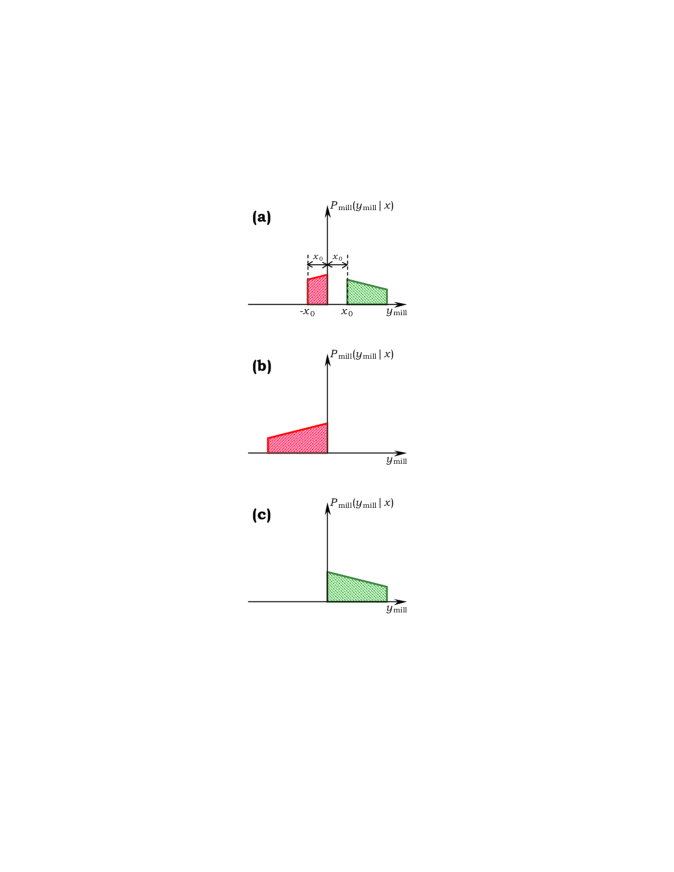
Figure 7: Three characteristic types of the asymmetry generating component of the conditional probability distribution: market mill (a), contrarian (b) and trend-following (c).

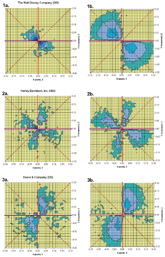
Figure 8: Model individual portraits (1b, 2b, 3b) versus market data (1a, 2a, 3a).

References

- [1] A. Leonidov, V. Trainin, A. Zaitsev, ”On collective non-gaussian dependence patterns in high frequency financial data”, ArXiv:physics/0506072
- [2] A. Leonidov, V. Trainin, A. Zaitsev, S. Zaitsev, ”Market Mill Dependence Pattern in the Stock Market: Asymmetry Structure, Nonlinear Correlations and Predictability”, arXiv:physics/0601098.
- [3] A. Leonidov, V. Trainin, A. Zaitsev, S. Zaitsev, ”Market Mill Dependence Pattern in the Stock Market: Distribution Geometry, Moments and Gaussization”, arXiv:physics/0603103.
- [4] A. Leonidov, V. Trainin, A. Zaitsev, S. Zaitsev, ”Market Mill Dependence Pattern in the Stock Market: Individual Portraits”, arXiv:physics/0605138.
- [5] A. Leonidov, V. Trainin, A. Zaitsev, S. Zaitsev, ”Market Mill Dependence Pattern in the Stock Market: Modeling of Predictability and Asymmetry via Multi-component Conditional Distribution”, Physica A 386 (2007), 240
- [6] B. Mandelbrot, ”Fractal and Multifractal Finance. Crashes and Long-dependence”, www.math.yale.edu/mandelbrot/webbooks/wb_fin.html
- [7] C.W. Granger, ”Long memory relationships and the aggregation of dynamical models”, Journal of Econometrics 14 (1980), 227-238
- [8] B. LeBaron, ”Stochastic volatility as a simple generator of apparent financial power laws and long memory”, Quantitative Finance 1 (2001), 621-631.
- [9] P.E. Lynch, G.O. Zumbach, ”Market heterogeneities and the causal struture of volatility”, Quantitative Finance 3 (2003), 320-331
- [10] L. Borland, J.-Ph. Bouchaud, ”On a multi-timescale statistical feedback model for volatility fluctuations”, ArXiv:physics/0507073
- [11] B. LeBaron, ”Time scales, agents, and empirical finance”, Medium Econometrische Toepassingen 14 (2006).
- [12] B. LeBaron, R. Yamamoto, ”Long-memory in an order-driven market”, Physica A 383 (2007), 85-89.
- [13] S.V. Panuykov, ”Theory of market fluctuations”, ArXiv:0804.4191(physics.soc-ph)
- [14] F. Lillo, J.D. Farmer, ”The long memory of the efficient market”, Studies in Nonlinear Dynamics and Econometrics, 8 (2004)
- [15] J.-P. Bouchaud, Y. Gefen, M. Potters, M. Wyart, ”Fluctuations and response in financial markets: the subtle nature of ’random’ price changes”, Quantitative Finance 4 (2004), 176-190
- [16] J.-P. Bouchaud, J. Kockelloren, M. Potters, ”Random walks, liquidity molasses and critical response in financial markets”, Quantitative Finance 6 (2006), 115-123
- [17] A. Kempf, O. Korn, ”Market depth and order size”, Journal of Financial Markets 2 (1999), 29
- [18] V. Plerou, X. Gabaix, P. Goikrishnan, H.E. Stanley, ”Quantifying stock price reponse to demand fluctuations”, Phys. Rev. E66 (2002), 027104
- [19] X. Gabaix, P. Goikrishnan, V. Plerou, H.E. Stanley, ”A theory of power-law distributions in financial markets fluctuations”, Nature, 423 (2003), 267