Relativistic multirank interaction kernels of the neutron-proton system

Abstract

The multirank separable kernels of the neutron-proton interaction for uncoupled $S$ and $P$ partial waves (with the total angular momentum $J$=0,1) are proposed. Two different methods of a relativistic generalization of initially nonrelativistic form factors parametrizing the kernel are considered. Using the constructed kernels the experimental data for phase shifts in the elastic neutron-proton scattering for the laboratory energy up to 3 GeV and low-energy parameters are described. The comparison of our results with other model calculations are presented.

1 Introduction

The problem of an adequate description of nuclear interactions arose many years ago. An important role in this task is played by the construction of the nucleon-nucleon interaction. The simplest way to investigate such interaction is to describe properties of the elastic neutron-proton ($np$) scattering and their bound state - deuteron. The latter can be considered through some reactions, such as the photodisintegration, the electrodisintegration etc.

There are a lot of works devoted to the description of the deuteron. The first models were based on the nonrelativistic Shr$\ddot{\rm o}$dinger equation (see, for example, [1, 2]). In numerous papers mesonic exchange currents, relativistic corrections were investigated and then were added to nonrelativistic solutions [3]-[16]. These approaches could describe properties of the deuteron such as binding energy, magnetic and quadruple momenta, electromagnetic form factors, tensor polarization and so on. However, with increasing of the precision of experimental data and obtaining new data at larger energies it became evident that it was necessary to take into account relativistic effects more carefully. And the consistency of the consideration of the deuteron breakup reactions demands also the final state interaction (FSI) between the outgoing nucleons to be taken into account.

One of the most consistent approaches is based on the solution of the Bethe-Salpeter (BS) equation [17]. In this case, we have to deal with a nontrivial integral equation. In addition to introduce the FSI of the final $np$ pair the BS equation for the continuous state should be solved. There is no method to get its exact solution. So various approximations were worked out. At present, the most known and developed approaches are the so-called quasipotential [18]-[29].

They consist in the simplification of the equations under consideration by some assumption. In most cases it means the deliverance from the relative energy, according to some physical reasons. For example, one of the particles is supposed on-mass-shell [27], or the time coordinates of particles are made equal [26], etc. There is another approach called the light front (LF) dynamics which was successfully developed and applied to explain the electromagnetic properties of the deuteron. In this approach, the state vector describing the system is expanded by Fock components defined on a hypersphere in the four-dimensional space-time. The LF dynamics approach is intuitively appealing, since it is formally close to the nonrelativistic description in terms of the Hamiltonian and state vectors can be directly interpreted as wave functions (see, for example, review [16]). The equivalence between LF dynamics and BS approaches was a subject of discussions presented in [16, 30] and references therein.

An alternative approach based on the exact solution of the BS equation is to use the separable ansatz for the interaction kernel in the BS equation [30]. In this case we can transform an integral equation to a system of linear equations. Parameters of the kernel are fitted by the description of phase shifts for respective partial states and low-energy parameters.

First separable parametrizations were worked out within nonrelativistic models. The form factors in the interaction kernel had no poles on a real axis in the relative energy complex plane [31, 32]. However, after the construction of a relativistic generalization such poles appeared [30]. In some cases they do not prevent to perform the calculations. As an example, such parametrizations are successfully used in the consideration of the deuteron photodisintegration [33], elastic electron-deuteron scattering, deuteron electrodisintegration on the threshold, and the deep inelastic scattering [30]. However, at high energies, one would have to deal with several thresholds corresponding to the production of one, two and more mesons of different types. This is clearly not feasible. A more practical approach is to employ phenomenological covariant separable kernel, which do not exhibit the meson-production thresholds, and can even be constructed in a singularity-free fashion, with the form factors chosen in the present paper and our Wick-rotation prescription. Thus, an accurate description of on-shell nucleon-nucleon data is possible, up to quite high energies. One then hopes that the used separable interactions also have a reasonable off-shell behaviour, so that realistic applications to other reactions can be done. The parametrization like that was proposed in [34]. In our previous works [35, 36], we constructed the one-rank interaction kernel of the same type. Due to the simplicity it works till the laboratory energy $\mbox{$T_{\rm Lab}$}\sim$1 GeV except the simplest partial wave ${}^{1}P_{1}^{+}$ where it gives satisfactory results for all available experimental data. In the present work, we develop this approach increasing the rank of the kernels and trying to describe the data for the phase shifts of uncoupled partial states in the energy range up to 3 GeV taken from the SAID program (http://gwdac.phys.gwu.edu). In future we plan to use these kernels in relativistic calculations of the deuteron electrodisintegration far from the threshold.

It should be emphasized that in this paper the new kernel is fitted to describe the neutron-proton elastic scattering data only. The description of the proton-proton scattering is a separate problem which requires specific methods of calculation. Our aim was to construct the separable kernels suitable for consideration of the scattered ${}^{1}P_{1},^{3}P_{0},^{3}P_{1},^{1}S_{0}$ states of the neutron-proton system.

The paper is organized as follows. In Section 2, the general Bethe-Salpeter formalism is considered. The used separable kernel is described in Section 3. Section 4 is devoted to the methods of a relativistic generalization of nonrelativistic Yamaguchi- and Tabakin-type form factors. In Section 5, the pole structure of the obtained relativistic expressions is analyzed. The parametrizations for definite partial channels are presented in Section 6. In Section 7, the scheme of performing numerical calculations is offered. The obtained results and the comparison with other model calculations are discussed in Section 8. In conclusion, in Section 9, the fields of application of the constructed kernels is briefly outlined.

2 Bethe-Salpeter formalism

Within the relativistic field theory, the elastic NN scattering can be described by the scattering $T$ matrix which satisfies the inhomogeneous BS equation. In momentum space, the BS equation for the $T$ matrix can be (in terms of the relative four-momenta $p^{\prime}$ and $p$ and the total four-momentum $P$) represented as:

$$T(p^{\prime},p;P)=V(p^{\prime},p;P)+\frac{i}{4\pi^{3}}\int d^{4}k\,V(p^{\prime},k;P)\,S_{2}(k;P)\,T(k,p;P),$$ (1)

where $V(p^{\prime},p;P)$ is the interaction kernel and $S_{2}(k;P)$ is the free two-particle Green function

$$S_{2}^{-1}(k;P)=\bigl{(}\tfrac{1}{2}\>P\cdot\gamma+{k\cdot\gamma}-m\bigr{)}^{(1)}\bigl{(}\tfrac{1}{2}\>P\cdot\gamma-{k\cdot\gamma}-m\bigr{)}^{(2)},$$

$\gamma$ are the Dirac gamma-matrices. The square of the total momenta $s=(p_{1}+p_{2})^{2}$ and the relative momentum $p=(p_{1}-p_{2})/2$ [$p^{\prime}=(p_{1}^{\prime}-p_{2}^{\prime})/2$] are defined via the nucleon momenta $p_{1},~{}p_{2}$ [$p_{1}^{\prime},~{}p_{2}^{\prime}$] of initial [final] nucleons.

To perform the partial-wave decomposition of the BS equation (1), we introduce relativistic two-nucleon basis states $|aM\rangle\equiv|\pi,\,{}^{2S+1}L_{J}^{\rho}M\rangle$, where $S$ denotes the total spin, $L$ is the orbital angular momentum, and $J$ is the total angular momentum with the projection $M$; relativistic quantum numbers $\rho$ and $\pi$ refer to the relative-energy and spatial parity with respect to the change of sign of the relative energy and spatial vector, respectively. Then the partial-wave decomposition of the $T$ matrix in the center-of-mass frame (c.m.) has the following form:

$$T_{\alpha\beta,\gamma\delta}(p^{\prime},p;{P_{(0)}})$$

$$=\sum_{JMab}({\cal Y}_{aM}(-{{\bf p}^{\prime}})U_{C})_{\alpha\beta}\otimes(U_{C}{\cal Y}^{{\dagger}}_{bM}({{\bf p}}))_{\delta\gamma}\ T_{ab}(p_{0}^{\prime},|{\bf p}^{\prime}|;p_{0},|{\bf p}|;s),$$ (2)

where $U_{C}=i\gamma^{2}\gamma^{0}$ is the charge conjugation matrix; the total momentum of the colliding nucleons in c.m. is denoted by $P_{(0)}$. Greek letters $(\alpha,\beta)$ and $(\gamma,\delta)$ in Eq.(2) refer to spinor indices and label particles in the initial and final states, respectively. It is convenient to represent the two-particle states in terms of matrices. To this end, the Dirac spinors of the second nucleon are transposed. At this stage $T$ is $16\times 16$ matrix in spinor space which, sandwiched between Dirac spinors and traced, yields the corresponding transition matrix elements between $SLJ$-states.

The spin-angular momentum functions ${\cal Y}_{aM}({{\bf p}})$ are expressed in terms of the positive- and negative-energy Dirac spinors $u^{\rho=\pm,\,1/2}_{m}$, the spherical harmonics $Y_{L{m_{L}}}$ and Clebsch-Gordan coefficients $C_{j_{1}m_{1}j_{2}m_{2}}^{j\>m}$:

$${\cal Y}_{JM:LS{\rho}}({\bf p})U_{C}$$

$$= i^{L}\sum_{m_{L}m_{S}m_{1}m_{2}\rho_{1}\rho_{2}}C_{\frac{1}{2}\rho_{1}\frac{1}{2}\rho_{2}}^{S_{\rho}{\rho}}C_{Lm_{L}Sm_{S}}^{JM}C_{\frac{1}{2}m_{1}\frac{1}{2}m_{2}}^{Sm_{S}}\times$$ (3)

$$~{}~{}~{}~{}~{}~{}~{}~{}~{}~{}~{}~{}~{}~{}~{}~{}~{}Y_{L{m_{L}}}({\bf p}){u^{\rho_{1}}_{m_{1}}}^{(1)}({\bf p}){{u^{\rho_{2}}_{m_{2}}}^{(2)}}^{T}(-{\bf p}).$$

The superscripts in Eq.(3) refer to particles (1) and (2). To derive the matrix elements between $a$-states, the ortonormalization condition for the functions ${\cal Y}_{aM}({{\bf p}^{\prime}})$ should be used:

$$\int\!d\varphi_{{\bf p}}\>d(\cos\theta_{{\bf p}})\,{\rm Tr}\left\{{\cal Y}^{{\dagger}}_{aM}({{\bf p}}){\cal Y}_{a^{\prime}M^{\prime}}({{\bf p}})\right\}\hskip 170.71652pt$$

$$\equiv\int\!d\varphi_{{\bf p}}\>d(\cos\theta_{{\bf p}})({\cal Y}^{{\dagger}}_{aM}({{\bf p}}))_{\beta\alpha}({\cal Y}_{a^{\prime}M^{\prime}}({{\bf p}}))_{\alpha\beta}=\delta_{aa^{\prime}}\delta_{MM^{\prime}},$$ (4)

where partial states $a$ and $a^{\prime}$ belong to the same partial channel.

The partial-wave decomposition for the interaction kernel $V$ of the BS equation (1) can be written analogously to Eq.(2):

$$V_{\alpha\beta,\gamma\delta}(p^{\prime},p;P_{(0)})$$

$$=\sum_{abM}({\cal Y}_{aM}(-{{\bf p}^{\prime}})U_{C})_{\alpha\beta}\otimes(U_{C}{\cal Y}^{{\dagger}}_{bM}({{\bf p}}))_{\delta\gamma}\ V_{ab}(p_{0}^{\prime},|{\bf p}^{\prime}|;p_{0},|{\bf p}|;s).$$ (5)

Applying the condition (4), we can obtain a system of linear integral equations for the off-shell partial-wave amplitudes:

$$T_{ab}(p_{0}^{\prime},|{\bf p}^{\prime}|;p_{0},|{\bf p}|;s)=V_{ab}(p_{0}^{\prime},|{\bf p}^{\prime}|;p_{0},|{\bf p}|;s)\hskip 142.26378pt$$ (6)

$$\hskip 108.12047pt+\frac{i}{4\pi^{3}}\sum_{cd}\int\limits_{-\infty}^{+\infty}\!dk_{0}\int\limits_{0}^{\infty}\!{\bf k}^{2}d|{\bf k}|\,V_{ac}(p_{0}^{\prime},|{\bf p}^{\prime}|;k_{0},|{\bf k}|;s)$$

$$\hskip 108.12047pt\times\,S_{cd}(k_{0},|{\bf k}|;s)\,T_{db}(k_{0},|{\bf k}|;p_{0},|{\bf p}|;s),$$

where the two-particle propagator $S_{ab}$ depends only on $\rho$-spin indices.

We use the normalization condition for the $T$ matrix in the on-mass-shell form for the singlet case:

$$T_{ll}(s)\equiv T_{ll}(0,\bar{p};0,\bar{p};s)=-\frac{16\pi}{\sqrt{s}\sqrt{s-4m^{2}}}\exp\{i\delta_{l}\}\sin\delta_{l},$$ (7)

where $\bar{p}\equiv|{\bar{\bf p}|}=\sqrt{s/4-m^{2}}=\sqrt{m\mbox{$T_{\rm Lab}$}/2}$ is the on-mass-shell momentum, $m$ is a nucleon mass. In Eq.(7) $l$ denotes ${}^{S}L_{J}$ states for simplicity. Low-energy parameters, the scattering length $a_{0}$, and the effective range $r_{0}$ are derived from the expansion of the $T$-matrix into a series of $\bar{p}$-terms, according to [37]:

$$\bar{p}\cot\delta_{l}(s)=-\frac{1}{a_{0}^{l}}+\frac{r_{0}^{l}}{2}\bar{p}^{2}+{\cal O}(\bar{p}^{3}).$$ (8)

To solve the equations for the $T$ matrix and BS amplitude, we should use some assumption for the interaction kernel.

3 A separable kernel

We assume that the interaction kernel $V$ conserves parity, total angular momentum $J$ and its projection, and isotopic spin. Due to the tensor nuclear force, the orbital angular momentum $L$ is not conserved. Moreover, the negative-energy two-nucleon states are switched off, which leads to the total spin $S$ conservation. The partial-wave-decomposed BS equation is therefore reduced to the following form:

$$T_{l^{\prime}l}(p_{0}^{\prime},|{\bf p}^{\prime}|;p_{0},|{\bf p}|;s)=V_{l^{\prime}l}(p_{0}^{\prime},|{\bf p}^{\prime}|;p_{0},|{\bf p}|;s)\hskip 142.26378pt$$ (9)

$$+\frac{i}{4\pi^{3}}\sum_{l^{\prime\prime}}\int\limits_{-\infty}^{+\infty}\!dk_{0}\int\limits_{0}^{\infty}\!{\bf k}^{2}d|{\bf k}|\,\frac{V_{l^{\prime}l^{\prime\prime}}(p_{0}^{\prime},|{\bf p}^{\prime}|;k_{0},|{\bf k}|;s)\,T_{l^{\prime\prime}l}(k_{0},|{\bf k}|;p_{0},|{\bf p}|;s)}{(\sqrt{s}/2-E_{{\bf k}}+i\epsilon)^{2}-k_{0}^{2}},$$

where $l=l^{\prime}=J$ for spin-singlet and uncoupled spin-triplet states.

Supposing the separable (rank $N$) ansatz for the kernel of the NN interaction:

$$V_{l^{\prime}l}(p_{0}^{\prime},|{\bf p}^{\prime}|;p_{0},|{\bf p}|;s)=\sum_{i,j=1}^{N}\lambda_{ij}(s)g_{i}^{[l^{\prime}]}(p_{0}^{\prime},|{\bf p}^{\prime}|)g_{j}^{[l]}(p_{0},|{\bf p}|),$$ (10)

where the form factors $g_{j}^{[l]}$ represent the model functions, we can obtain the solution of equation (3) in a similar separable form for the $T$ matrix:

$$T_{l^{\prime}l}(p_{0}^{\prime},|{\bf p}^{\prime}|;p_{0},|{\bf p}|;s)=\sum_{i,j=1}^{N}\tau_{ij}(s)g_{i}^{[l^{\prime}]}(p_{0}^{\prime},|{\bf p}^{\prime}|)g_{j}^{[l]}(p_{0},|{\bf p}|),$$ (11)

where

$$\tau_{ij}(s)=1/(\lambda_{ij}^{-1}(s)+h_{ij}(s)),$$ (12)

$$h_{ij}(s)=-\frac{i}{4\pi^{3}}\sum_{l}\int dk_{0}\int{\bf k}^{2}d|{\bf k}|\frac{g_{i}^{[l]}(k_{0},|{\bf k}|)g_{j}^{[l]}(k_{0},|{\bf k}|)}{(\sqrt{s}/2-E_{{\bf k}}+i\epsilon)^{2}-k_{0}^{2}},$$ (13)

$\lambda_{ij}(s)$ is a matrix of model parameters.

The form factors $g_{i}^{[l]}$ used in the separable representation of the interaction kernel (10) are obtanied by a relativistic generalization of the initially nonrelativistic Yamaguchi-type functions depending on the three-dimensional squared momentum $|{\mbox{\boldmath$p$}}|$. There are two methods to derive covariant relativistic generalizations of nonrelativistic form factors. They are considered in the next section.

Calculating the $T$ matrix we can connect the parameters of the internal kernel with observables.

4 Methods of a covariant relativistic generalization

In this section, two methods of a covariant relativistic generalization of the Yamaguchi- and Tabakin-type functions are presented.

1. One of the common methods is to replace three-momentum squared by four-momentum squared:

   $${\bf p}^{2}\to-p^{2}=-p_{0}^{2}+{\bf p}^{2}.$$ (14)

   This formal procedure converts three-dimensional functions to covariant four-dimensional ones.

2. The other method is based on the introduction of the formal four-vector $Q$ via the relative $p$ and total $P$ four-momenta of the two-body system by the following relation:

   $$Q=p-\frac{P\cdot p}{s}P,$$ (15)

   with the total momentum squared $s=P^{2}$.

Note that in the two-particle center-of-mass system where $P=(\sqrt{s},{\mbox{\boldmath$0$}})$ the four-vector $Q$ is defined by the components $Q=(0,{\bf p})$ and, thus,

$${\bf p}^{2}=-Q^{2}$$ (16)

can be formally converted to the Lorentz invariant.

Let us consider the methods described above as applied to the nonrelativistic Yamaguchi-type function

$$g(|{\bf p}|)=\frac{1}{{\bf p}^{2}+\beta^{2}}.$$ (17)

In the first case, using the substitution (14) we obtain the covariant function in the form:

$$g_{p}(p,P)=\frac{1}{-p^{2}+\beta^{2}}\stackrel{{\scriptstyle\rm c.m.}}{{\longrightarrow}}\frac{1}{-p_{0}^{2}+{\bf p}^{2}+\beta^{2}+i\epsilon}.$$ (18)

In the second case, we use relation (16) and obtain the function:

$$g_{Q}(p,P)=\frac{1}{-Q^{2}+\beta^{2}}\stackrel{{\scriptstyle\rm c.m.}}{{\longrightarrow}}\frac{1}{{\bf p}^{2}+\beta^{2}}.$$ (19)

The presented functions have rather different properties in the relative energy $p_{0}$ complex plane in c.m. The function $g_{p}$ has two poles on the real axis for $p_{0}$ at $\pm\sqrt{{\bf p}^{2}+\beta^{2}}\mp i\epsilon$ while the function $g_{Q}$ has no poles on it.

In practical calculations of the reactions with the high momentum transfer the $p_{0}$ integration can lead to singular expressions in functions $g_{p,Q}$ on $|{\bf p}|$ or $\cos{\theta_{{\bf p}}}$. This problem can be easily solved by calculating the $|{\bf p}|$ or $\cos{\theta_{{\bf p}}}$ principal value integral. However, another form of functions $g_{p,Q}$ with odd powers in the denominator leads to nonintegrable singularities. Therefore, we introduce functions $g_{p,Q}$ of type without poles on the real axis in the relative energy $p_{0}$ complex plane. As an example of a function like that we introduce the covariant form factors in the following form (see also section 3 of [35]):

$$g_{p}(p,P)=\frac{p_{c}-p^{2}}{(p^{2}-\beta^{2})^{2}+\alpha^{4}}\stackrel{{\scriptstyle\rm c.m.}}{{\longrightarrow}}\frac{p_{c}-p_{0}^{2}+{\bf p}^{2}}{(p_{0}^{2}-{\bf p}^{2}-\beta^{2})^{2}+\alpha^{4}},$$ (20)

and in the second case we use relation (16) and obtain the function

$$g_{Q}(p,P)=\frac{p_{c}-Q^{2}}{(Q^{2}-\beta^{2})^{2}+\alpha^{4}}\stackrel{{\scriptstyle\rm c.m.}}{{\longrightarrow}}\frac{p_{c}+{\bf p}^{2}}{({\bf p}^{2}+\beta^{2})^{2}+\alpha^{4}}.$$ (21)

We note that the function $g_{Q}$ still has no poles on the $p_{0}$ real axis while $g_{p}$ has poles at $p_{0}$: $\pm\sqrt{{\bf p}^{2}+\beta^{2}+i\alpha^{2}},\quad\pm\sqrt{{\bf p}^{2}+\beta^{2}-i\alpha^{2}}$.

The two methods of a covariant relativistic generalization described above can be investigated by solving the Bethe-Salpeter equation for specific partial states.

5 Pole structure of the BS solution

The solution of the Bethe-Salpeter equation with the separable kernel of interaction contains the function $h_{ij}$ (13). To simplify the investigation of the pole structure, let us consider $h_{ij}$ for the one-rank kernel ($i=j=1$) for single $l$ state. Then the value to be calculated is $h(s)$:

$$h(s)=-\frac{i}{4\pi^{3}}\int dp_{0}\int{\bf p}^{2}d|{\bf p}|\frac{{g(p_{0},|{\bf p}|)^{2}}}{{(\sqrt{s}/2-E_{{\bf p}}+i\epsilon)^{2}-p_{0}^{2}},}.$$ (22)

To obtain the function $h(s)$, the two-dimensional integral on $p_{0}$ and $|{\bf p}|$ should be calculated. To perform the integration over $p_{0}$, the Cauchy theorem is used. As it can be seen from Eq.(22), there are two types of singularities on the real axis in the $p_{0}$ complex plane: one is poles of the function $S(p;s)$:

$$p^{(1,2)}_{0}=\pm\sqrt{s}/2\mp E_{{\bf p}}\pm i\epsilon,$$ (23)

and the other is poles of the function $g(p)$.

The function $g_{p}$ has four poles:

$$p^{(3,4)}_{0}=\pm\sqrt{{\bf p}^{2}+\beta^{2}+i\alpha^{2}},$$

$$p^{(5,6)}_{0}=\pm\sqrt{{\bf p}^{2}+\beta^{2}-i\alpha^{2}},$$ (24)

and to perform the $p_{0}$ integration, residues in three poles of Eqs.(23) and (24) should be calculated. These calculations are performed analytically. This procedure is worthy of a special discussion. All poles and the contour of integration are pictured in Fig.1. The idea how to choose the contour appeared owing to [38, 39]. It consists in that the contour must envelope the poles from form factors which will be inside the standard contour after the $\alpha\rightarrow 0$ limit. ”Standard” means the one used in the quantum field theory calculations with a propagator which has poles only on the real axis in the $p_{0}$ complex plane; one of them is rounded from below and the other, from above. So the path of integration is defined by an appropriate contour for the propagator. The calculation over the presented path leads to the pure real contribution from the form factor poles and, therefore, to the unitary $T$ matrix. We also obtain a correct transition to ordinary form factors of type $g\sim 1/(p_{0}^{2}-{\bf p}^{2}-\beta^{2})^{2}$ in the $\alpha\rightarrow 0$ limit.

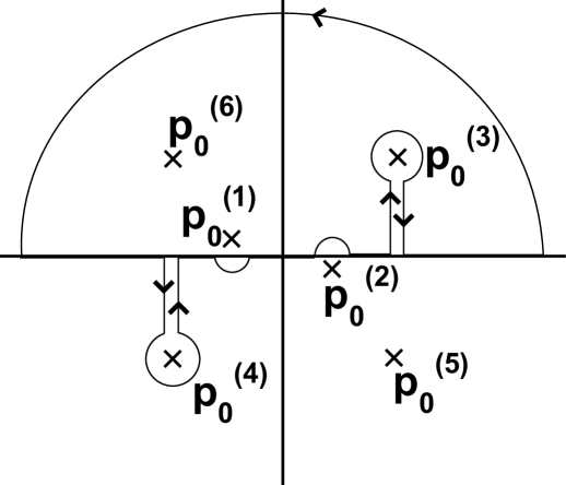
Figure 1: Contour for integration over $p_{0}$.

The function $g_{Q}$ has no poles on the $p_{0}$ real axis and, therefore, the only poles of Eq.(23) should be taken into account. The result for $h(s)$ can be written as:

$$h(s)=\frac{1}{2\pi^{2}}\int{\bf p}^{2}d|{\bf p}|\frac{g_{Q}(0,|{\bf p}|)^{2}}{\sqrt{s}-2E_{{\bf p}}+i\epsilon}.$$ (25)

This equation formally coincides with that could be obtained within the Blankenbeckeler-Sugar-Logunov-Tavkhelidze (BSLT) approximation [18, 19] which consists in replacing the Green function in Eq.(22) by the expression

$$S_{BSLT}(p;s)=-2\pi i(\sqrt{s}-2E_{{\bf p}}+i\epsilon)^{-1}\delta(p_{0}).$$ (26)

Although the solutions of the equation with functions $g_{Q}$ and within the BSLT approximation coincide in c.m., the difference becomes evident when the reaction with the two-particle system is considered. In that case, the arguments of the function $g_{Q}$ are calculated with the help of the Lorentz transformations in the system different from c.m. The functions become similar to $g_{p}$ but with a more complicated dependence of the $p$ argument. In our calculations we prefer to use the first method of relativization. The reason is in that reaction we are planning to consider in future (namely, electrodisintegration) these transformations could lead to the appearance of additional poles in the calculated expressions. However, in this work the comparison of results for phase shifts and low-energy parameters is presented for both cases.

In following two sections some separable presentations of the interaction kernel for the partial waves with $J=0,1$ are considered. Form factors are constructed by the relativization procedure, according to the first method. The functions with $Q$ can be obtained from them by the change $p^{2}\rightarrow Q^{2}$.

6 Separable presentations of the kernel

We consider the partial states using the separable kernels with modified Yamaguchi-type functions of $N$ rank (MY$N$, MYQ$N$).

6.1 Two-rank kernel for $P$ states: ${}^{3}P_{0}^{+}$, ${}^{1}P_{1}^{+}$, ${}^{3}P_{1}^{+}$

For the description of the $P$ partial waves the two-rank separable kernel of interaction with the modified Yamaguchi-type functions is used. Its form factors are written as:

$$g^{[P]}_{1}(p)=\frac{\sqrt{-p_{0}^{2}+{\bf p}^{2}}}{(p_{0}^{2}-{\bf p}^{2}-\beta_{1}^{2})^{2}+\alpha_{1}^{4}},$$ (27)

$$g^{[P]}_{2}(p)=\frac{\sqrt{(-p_{0}^{2}+{\bf p}^{2})^{3}}(p_{c2}-p_{0}^{2}+{\bf p}^{2})}{((p_{0}^{2}-{\bf p}^{2}-\beta_{2}^{2})^{2}+\alpha_{2}^{4})^{2}}.$$

6.2 Three-rank kernel for ${}^{1}S_{0}^{+}$ state

The investigation we performed demonstrates a bad description of phase shifts for ${}^{1}S_{0}^{+}$ partial state by the two-rank kernel. It is not much better than by the one-rank kernel [35]. So for this special case the three-rank interaction kernel was elaborated. Its form factors have the following form:

$$g^{[S]}_{1}(p)=\frac{(p_{c1}-p_{0}^{2}+{\bf p}^{2})}{(p_{0}^{2}-{\bf p}^{2}-\beta_{1}^{2})^{2}+\alpha_{1}^{4}},$$ (28)

$$g^{[S]}_{2}(p)=\frac{(p_{0}^{2}-{\bf p}^{2})(p_{c2}-p_{0}^{2}+{\bf p}^{2})^{2}}{((p_{0}^{2}-{\bf p}^{2}-\beta_{2}^{2})^{2}+\alpha_{2}^{4})^{2}},$$

$$g^{[S]}_{3}(p)=\frac{(p_{0}^{2}-{\bf p}^{2})}{(p_{0}^{2}-{\bf p}^{2}-\beta_{3}^{2})^{2}+\alpha_{3}^{4}}.$$

The functions are numerated by angular momenta $L=0([S]),1([P])$. The numerator with $p_{c}$ in $g_{2}^{[P]}$ and $g^{[S]}_{1,2}$ is introduced to compensate an additional dimension in the denominator to provide the total dimension as GeV^-2 [35].

7 Calculations and results

Using the $np$ scattering data we analyze the parameters of the separable kernels distinguishing three different cases:

1. There are no sign change in phase shifts or bound state (${}^{1}P_{1}^{+},~{}^{3}P_{1}^{+}$ partial states). In this case

   $$\lambda_{ij}(s)=\bar{\lambda}_{ij}=const.$$ (29)

   This is sufficient for most of the higher partial waves.

2. One sign change and no bound state (${}^{1}S_{0}^{+},~{}^{3}P_{0}^{+}$ partial states). In this case the energy-dependent expression for $\lambda_{l}(s)$ is used (see [34] and references therein):

   $$\lambda_{ij}(s)=(s_{0}-s)\bar{\lambda}_{ij},$$ (30)

   Here the parameter $s_{0}$ is introduced to reproduce the sign change in the phase shifts at the position of the experimental value for the kinetic energy $T_{\rm Lab}$ where they are equal to zero. It is added to the other parameters of the kernel.

The calculation of the parameters is performed by using Eqs.(7), (8) and expressions given in two previous sections to reproduce experimental values for all available data from the SAID program (http://gwdac.phys.gwu.edu) for the phase shifts. The the low-energy scattering parameters are taken from [40].

The calculations are performed in two independent ways. The first one is based on using the Cauchy theorem for the integration over $p_{0}$ component of the nucleon four-momentum. The integration over $|{\mbox{\boldmath$p$}}|$ is performed numerically. The second one is based on using the Wick rotation [39]. In this case the contour of integration Fig.1 is deformed as depicted on Fig.2. All integrals are calculated numerically with the technique elaborated in the paper [41].

Figure 2: Contour for integration over $p_{0}$ after the Wick rotation.

Now we find the introduced parameters of the kernel:

1. For $P$ waves the minimization procedure for the function

   $$\chi^{2}=\sum\limits_{i=1}^{n}(\delta^{\rm exp}(s_{i})-\delta(s_{i}))^{2}/(\Delta\delta^{\rm exp}(s_{i}))^{2}$$ (31)

   is used. Here $n$ is a number of available experimental points.

2. For the ${}^{1}S_{0}^{+}$ wave the values of the scattering length $a$ is also included into the minimization procedure

   $$\chi^{2}=\sum\limits_{i=1}^{n}(\delta^{\rm exp}(s_{i})-\delta(s_{i}))^{2}/(\Delta\delta^{\rm exp}(s_{i}))^{2}+(a^{\rm exp}-a)^{2}/(\Delta a^{\rm exp})^{2}.$$ (32)

The effective range $r_{0}$ is calculated via the obtained parameters and compared with the experimental value $r_{0}^{\rm exp}$.

The description of $P$ waves by the two-rank kernel is denoted by MY2 for the first case of a relativization procedure; MYQ2, for the second one. For the ${}^{1}S_{0}^{+}$ partial state the notation MY3 and MYQ3, respectively, are used.

The calculated parameters of the considered kernels are listed in Tables 1 and 2 (here the values of $s_{0}$ are presented, too). In Table 3, the calculated low-energy scattering parameters for the ${}^{1}S_{0}^{+}$ wave are compared with their experimental values.

In Figs.3-6, the results of the phase shift calculations are compared with experimental data (the used notation is described in the following Section 8) and two alternative descriptions by CD-Bonn [42] and SP07 [43]. In the discussion of the ${}^{1}S_{0}^{+}$ channel the nonrelativistic Graz II [31], as an alternative model with a separable kernel, is also presented.

Table 1: Parameters of the two-rank kernel with modified Yamaguchi functions for $P$ waves.

		MY2
	${}^{1}P_{1}^{+}$	${}^{3}P_{0}^{+}$	${}^{3}P_{1}^{+}$
$\bar{\lambda}_{11}^{{\phantom{1}}^{\phantom{1}}}$ (GeV4)	0.05412952	-923.8881	0.06125619
$\bar{\lambda}_{12}$ (GeV4)	1.925	-102.0961	2.068215
$\bar{\lambda}_{22}$ (GeV4)	7.975	4.346553	24.48148
$\beta_{1}$ (GeV)	0.1244769	0.958602	0.1224502
$\beta_{2}$ (GeV)	0.6228701	1.897255	0.5822389
$\alpha_{1}$ (GeV)	0.2	0.759970	0.2107709
$\alpha_{2}$ (GeV)	0.5984991	0.687087	0.5927882
$p_{c2}$ (GeV2)	1.035	-133.2385	0.9476951
$s_{0}$ (GeV2)		3.8682
		MYQ2
	${}^{1}P_{1}^{+}$	${}^{3}P_{0}^{+}$	${}^{3}P_{1}^{+}$
$\bar{\lambda}_{11}^{{\phantom{1}}^{\phantom{1}}}$ (GeV4)	0.3086486	-55.88270	0.07648584
$\bar{\lambda}_{12}$ (GeV4)	1.606382	-763.1649	1.567463
$\bar{\lambda}_{22}$ (GeV4)	-5.797411	-5325.327	21.25497
$\beta_{1}$ (GeV)	0.2150637	0.5008744	0.2109235
$\beta_{2}$ (GeV)	0.9582849	2.4269161	0.4260685
$\alpha_{1}$ (GeV)	0.2	0.6863803	0.2
$\alpha_{2}$ (GeV)	0.2	0.2	0.2
$p_{c2}$ (GeV2)	12.47736	5.866078	0.007380749
$s_{0}$ (GeV2)		3.8682

Table 2: Parameters of the three-rank kernel with modified Yamaguchi functions for ${}^{1}S_{0}^{+}$ state.

		MY3
$\bar{\lambda}_{11}^{{\phantom{1}}^{\phantom{1}}}$ (GeV2)	-0.2922173		$\beta_{1}$ (GeV)	0.7018063
$\bar{\lambda}_{12}$ (GeV2)	-3.953624		$\beta_{2}$ (GeV)	4.381178
$\bar{\lambda}_{13}$ (GeV2)	1.035416		$\beta_{3}$ (GeV)	1.137604
$\bar{\lambda}_{22}$ (GeV2)	-11268.52		$\alpha_{1}$ (GeV)	1.297282
$\bar{\lambda}_{23}$ (GeV2)	331.1130		$\alpha_{2}$ (GeV)	4.612956
$\bar{\lambda}_{33}$ (GeV2)	70.37369		$\alpha_{3}$ (GeV)	0.6752485
$s_{0}$ (GeV2)	4.0279		$p_{c1}$ (GeV2)	38.20462
			$p_{c2}$ (GeV2)	34.53211
		MYQ3
$\bar{\lambda}_{11}^{{\phantom{1}}^{\phantom{1}}}$ (GeV2)	723.7399		$\beta_{1}$ (GeV)	2.463736
$\bar{\lambda}_{12}$ (GeV2)	550.4827		$\beta_{2}$ (GeV)	1.266692
$\bar{\lambda}_{13}$ (GeV2)	-1583.031		$\beta_{3}$ (GeV)	7.714815
$\bar{\lambda}_{22}$ (GeV2)	132.7836		$\alpha_{1}$ (GeV)	3.752405
$\bar{\lambda}_{23}$ (GeV2)	-14.26609		$\alpha_{2}$ (GeV)	2.117966
$\bar{\lambda}_{33}$ (GeV2)	-26005.23		$\alpha_{3}$ (GeV)	1.338336
$s_{0}$ (GeV2)	4.0279		$p_{c1}$ (GeV2)	-44.84322
			$p_{c2}$ (GeV2)	247.2476

Table 3: The low-energy scattering parameters and for the singlet $(s)$ ${}^{1}S_{0}^{+}$ wave.

	$a_{s}$(fm)	$r_{0s}$(fm)
MY3	-23.750	2.70
MYQ3	-23.754	2.78
Experiment	-23.748(10)	2.75(5)

8 Discussion

In this section, the review of the results of our calculations with two methods of relativization is performed.

In. Fig.3, we can see that all of the calculations including nonrelativistic CD-Bonn give a quite good description of the ${}^{1}P_{1}^{+}$ state. In our previous works [35, 36], it was shown that the one-rank kernel is already sufficient to reproduce the phase shifts in this case. The reason is the simplicity of their behavior and the narrowness of the energy interval where they are known. So if the simplicity of the model to perform calculations in the ${}^{1}P_{1}^{+}$ state is preferable, it is sufficient to use the one-rank kernel. For the energies $\mbox{$T_{\rm Lab}$}>1.1$ GeV the resulting functions become very different. To make choice in favour of one of the parametrizations, it is necessary to have experimental data for larger energies.

In Fig.4, the results of the calculations for the ${}^{3}P_{0}^{+}$ partial state are depicted. The comparison of our and other model calculations demonstrates a reasonable agreement with the experimental data in the whole range of energies except the nonrelativistic CD-Bonn which works till $\mbox{$T_{\rm Lab}$}\sim 0.75$ GeV. The good description of the phase shifts in ${}^{3}P_{0}^{+}$ can also be archived by using the one-rank interaction kernel with extended Yamaguchi-type form factors (see [35, 36]). As in the previous case, the choice of the kernel is defined, by reasons of convenience, as applied to a specific problem.

The phase shift calculations for the ${}^{3}P_{1}^{+}$ partial state are presented in Fig.5. All models except CD-Bonn give various but acceptable within the limits of error results. The CD-Bonn works for $\mbox{$T_{\rm Lab}$}\leqslant 0.66$ GeV. As for our previous one-rank kernel, the increase of the rank allows us to improve the description and embrace all experimental data.

Our general conclusion about the description of $P$ states is that using the two-rank kernel allows to reproduce the phase shifts in good agreement with experimental data. If the simplicity is the main requirement of performing calculations, the one-rank kernel for ${}^{1}P_{1}^{+}$ and ${}^{3}P_{0}^{+}$ states and two-rank one for ${}^{3}P_{1}^{+}$ can be used. Here we talk about phases in the whole energy range for $T_{\rm Lab}$. However, if the use of a common interaction kernel is preferable, then calculations with two-rank interaction kernel should be done.

From Fig.6, where the results of calculations for ${}^{1}S_{0}^{+}$ are presented, it can be seen that CD-Bonn is quite good till $\mbox{$T_{\rm Lab}$}\sim 0.66$ GeV. All the other results are in agreement with measured phase shifts except Graz II which works for $\mbox{$T_{\rm Lab}$}\leqslant 2$ GeV. We succeed in an acceptable description at the cost of increasing the kernel’s rank. Kernels of lower ranks are proper only for energies $\mbox{$T_{\rm Lab}$}\leqslant$1 GeV.

From the presented figures the similarity of the calculations with the MY and MYQ form factors can be noted. Thus, as for the description of phase shifts and low-energy parameters there is no difference which variant of a relativistic generalization to choose. The choice should be dictated by the convenience of performing calculations within some concrete problem.

Figure 3: Phase shifts for the ${}^{1}P_{1}^{+}$ wave.

Figure 4: Phase shifts for the ${}^{3}P_{0}^{+}$ wave.

Figure 5: Phase shifts for the ${}^{3}P_{1}^{+}$ wave.

Figure 6: Phase shifts for the ${}^{1}S_{0}^{+}$ wave.

9 Conclusion

Using the multirank kernels (two-rank for $P$ waves, three-rank for the ${}^{1}S_{0}^{+}$ partial state) we have constructed an adequate description of all existent experimental data for phase shifts taken from SAID and low-energy parameters with capable accuracy.

The results for two different methods of a relativistic generalization of initially nonrelativistic Yamaguchi-type form factors were considered. As it was shown they lead to slightly different descriptions of phases and low-energy parameters. Hence, the choice of the concrete form of functions for performing calculations of any process is governed only by convenience.

In spite of the fact that the model functions have a simple form there are quite a few parameters in the description of the data. This is necessitated by introduction of an additional parameter $\alpha$ so that integrands containing form factors of the separable kernel could not have poles. In particular, using this type of kernels will make the numerical calculations of the electrodisintegration far from the threshold possible without resorting quasipotential or nonrelativistic models.

10 Acknowledgements

We are grateful to Drs. A.A. Goy and D.V. Shulga for their interest in this work. We would also like to thank Dr. Y. Yanev for computational advice and Professor G. Rupp for his leading questions and recommendations for a more precise formulation of the basis of our model.

References

- [1] G.E. Brown and A.D. Jackson, RX-707 (NORDITA).
- [2] J.F. Mathiot, Nucl. Phys. A 412 (1984) 201.
- [3] M. Gari, H. Hyuga, Z. Phys. A 277 (1976) 291.
- [4] M. Gari, H. Hyuga, Nucl. Phys. A 278 (1977) 372.
- [5] M. Gari, H. Hyuga, B. Sommer, Phys. Rev. C (1976) 14 2196.
- [6] V.V. Burov, V.N. Dostovalov, S.E. Suskov, Sov. J. Part. Nucl. 23 (1992) 317.
- [7] V.V. Burov, V.N. Dostovalov, S.E. Suskov, JETP Lett. 44 (1986) 457.
- [8] V.V. Burov, V.N. Dostovalov, Z. Phys. A 326 (1987) 245.
- [9] V.V. Burov, A.A. Goi, V.N. Dostovalov, Sov. J. Nucl. Phys. 45 (1987) 616.
- [10] W.Y.P. Hwang, G.E. Walker, Annals Phys. 159 (1985) 118.
- [11] A.O. Gattone, B. Goulard, W.Y.P. Hwang, Phys. Rev. C 31 (1985) 1430.
- [12] W.Y.P. Hwang, J.T. Londergan, G.E. Walker, Annals Phys. 149 (1983) 335.
- [13] W.Y.P. Hwang, T.W. Donnelly, Phys. Rev. C 33 (1986) 1381.
- [14] R.F. Wagenbrunn, W. Plessas, Few Body Syst. Suppl. 8 (1995) 181.
- [15] T. Wilbois, G. Beck, H. Arenhovel, Few Body Syst. 15 (1993) 39.
- [16] J. Carbonell, B. Desplanques, V.A. Karmanov, J.F. Mathiot, Phys. Rept. 300 (1998) 215, nucl-th/9804029.
- [17] E.E. Salpeter, H.A. Bethe, Phys. Rev. 84 (1951) 1232.
- [18] A.A. Logunov, A.N. Tavkhelidze, Nuovo Cim. 29 (1963) 380.
- [19] R. Blankenbecler, R. Sugar, Phys. Rev. 142 (1966) 1051.
- [20] V.G. Kadyshevsky, Nucl. Phys. B 6 (1968) 125.
- [21] F. Gross, Phys. Rev. 186 (1969) 1448.
- [22] W.W. Buck, F. Gross, Phys. Rev. D 20 (1979) 2361.
- [23] F. Gross, Nucl. Phys. A 358 (1981) 215c.
- [24] F. Gross, World Scientific (1991).
- [25] F. Gross, J.W. Van Orden, K. Holinde, Phys. Rev. C 45 (1992) 2094.
- [26] V. Pascalutsa, J.A. Tjon, Phys. Rev. C 61 (2000) 054003, nucl-th/0003050.
- [27] J. Adam, J., F. Gross, S. Jeschonnek, P. Ulmer, J. W. Van Orden, Phys. Rev. C66 (2002) 044003, nucl-th/0204068.
- [28] R.A. Gilman, F. Gross, J. Phys. G 28 (2002) R37, nucl-th/0111015.
- [29] M. Garcon, J.W. Van Orden, Adv. Nucl. Phys. 26 (2001) 293, nucl-th/0102049.
- [30] S.G. Bondarenko, V.V. Burov, A.V. Molochkov, G.I. Smirnov, H. Toki, Prog. Part. Nucl. Phys. 48 (2002) 449, nucl-th/0203069.
- [31] L. Mathelitsch, W. Plessas, M. Schweiger, Phys. Rev. C 26 (1982) 65.
- [32] J. Haidenbauer, W. Plessas, Phys. Rev. C 30 (1984) 1822.
- [33] S.G. Bondarenko, V.V. Burov, K.Y. Kazakov, D.V. Shulga, Phys. Part. Nucl. Lett. 1 (2004) 178, nucl-th/0402056.
- [34] K. Schwarz, J. Frohlich, H.F.K. Zingl, Acta Phys. Austriaca 53 (1981) 191.
- [35] S.G. Bondarenko, V.V. Burov, W.-Y. Pauchy Hwang, E.P. Rogochaya, JETP Lett. 87 (2008) 753, 0804.3525.
- [36] S.G. Bondarenko, V.V. Burov, E.P. Rogochaya, Y. Yanev, 0806.4866 (2008).
- [37] H.A. Bethe, Phys. Rev. 76 (1949) 38.
- [38] R.E. Cutkosky, P.V. Landshoff, D.I. Olive, J.C. Polkinghorne, Nucl. Phys. B 12 (1969) 281.
- [39] T.D. Lee, G.C. Wick, Nucl. Phys. B 9 (1969) 209.
- [40] O. Dumbrajs et al., Nucl. Phys. B 216 (1983) 277.
- [41] J. Fleischer, J.A. Tjon, Nucl. Phys. B 84 (1975) 375.
- [42] R. Machleidt, Phys. Rev. C 63 (2001) 024001, nucl-th/0006014.
- [43] R.A. Arndt, W.J. Briscoe, I.I. Strakovsky, R.L. Workman, Phys. Rev. C 76 (2007) 025209, 0706.2195.