ITP–UH–21/08

N=4 Mechanics, WDVV Equations and Polytopes

Olaf Lechtenfeld

Institut für Theoretische Physik, Leibniz Universität Hannover

$N{=}4$ superconformal $n$-particle quantum mechanics on the real line is governed by two prepotentials, $U$ and $F$, which obey a system of partial nonlinear differential equations generalizing the Witten-Dijkgraaf-Verlinde-Verlinde (WDVV) equation for $F$. The solutions are encoded by the finite Coxeter systems and certain deformations thereof, which can be encoded by particular polytopes. We provide $A_{n}$ and $B_{3}$ examples in some detail. Turning on the prepotential $U$ in a given $F$ background is very constrained for more than three particles and nonzero central charge. The standard ansatz for $U$ is shown to fail for all finite Coxeter systems. Three-particle models are more flexible and based on the dihedral root systems.

1 Conformal quantum mechanics: Calogero system

We are investigating systems of $n{+}1$ identical point particles with unit mass whose motion on the real line is governed by the Hamiltonian

$$H\ =\ {\textstyle\frac{1}{2}}p_{i}p_{i}\ +\ V_{B}(x^{1},\dots,x^{n+1})$$ (1.1)

and subject to the canonical quantization relations

$$[x^{i},p_{j}]\ =\ {\mathrm{i}}{\delta_{j}}^{i}\ .$$ (1.2)

Together with

$$D\ =\ -{\textstyle\frac{1}{4}}(x^{i}p_{i}+p_{i}x^{i})\qquad{\textrm{and}}\qquad K\ =\ {\textstyle\frac{1}{2}}x^{i}x^{i}\ ,$$ (1.3)

this Hamiltonian realizes an $so(1,2)$ conformal algebra

$$[D,H]\ =\ -{\mathrm{i}}H\ ,\quad[H,K]\ =\ 2{\mathrm{i}}D\ ,\quad[D,K]\ =\ {\mathrm{i}}K$$ (1.4)

if the potential is homogeneous of degree $-2$,

$$(x^{i}\partial_{i}+2)\,V_{B}\ =\ 0\ .$$ (1.5)

When demanding also permutation and translation invariance as well as admitting only two-body forces, the solution is uniquely given by the Calogero potential,

$$V_{B}\ =\ \sum_{i<j}{\textstyle\frac{g^{2}}{(x^{i}-x^{j})^{2}}}\ .$$ (1.6)

2 ${\cal N}{=}4$ superconformal extension: $su(1,1|2)$ algebra

Let us extend the algebra from $so(1,2)\simeq su(1,1)$ to the superalgebra $su(1,1|2)$ with central charge $C$ by enlarging the set of generators

$$(H,D,K)\ \to\ (H,D,K,Q_{\alpha},S_{\alpha},J_{a},C)\qquad\textrm{with}\quad\alpha=1,2\ ,\quad a=1,2,3\ ,\quad{(Q_{\alpha})}^{\dagger}{=}{\bar{Q}}^{\alpha}\ ,\quad{(S_{\alpha})}^{\dagger}{=}{\bar{S}}^{\alpha}$$

and imposing the nonvanishing (anti)commutators:

$$[D,H]=-\,{\mathrm{i}}H\ [H,K]=2{\mathrm{i}}D\$$

$$[D,K]=+{\mathrm{i}}K\ [J_{a},J_{b}]={\mathrm{i}}\epsilon_{abc}J_{c}\$$

$$\{Q_{\alpha},\bar{Q}^{\beta}\}=2H{\delta_{\alpha}}^{\beta}\ \{Q_{\alpha},\bar{S}^{\beta}\}=+2{\mathrm{i}}{{(\sigma_{a})}_{\alpha}}^{\beta}J_{a}-2D{\delta_{\alpha}}^{\beta}-\,{\mathrm{i}}C{\delta_{\alpha}}^{\beta}\$$

$$\{S_{\alpha},\bar{S}^{\beta}\}\ =2K{\delta_{\alpha}}^{\beta}\ \{\bar{Q}^{\alpha},S_{\beta}\}=-\,2{\mathrm{i}}{{(\sigma_{a})}_{\beta}}^{\alpha}J_{a}-2D{\delta_{\beta}}^{\alpha}+{\mathrm{i}}C{\delta_{\beta}}^{\alpha}\$$

$$[D,Q_{\alpha}]=-{\textstyle\frac{{\mathrm{i}}}{2}}Q_{\alpha}\ [D,S_{\alpha}]=+{\textstyle\frac{{\mathrm{i}}}{2}}S_{\alpha}\$$

$$[K,Q_{\alpha}]=+{\mathrm{i}}S_{\alpha}\ [H,S_{\alpha}]=-{\mathrm{i}}Q_{\alpha}\$$

$$[J_{a},Q_{\alpha}]=-{\textstyle\frac{1}{2}}{{(\sigma_{a})}_{\alpha}}^{\beta}Q_{\beta}\qquad\qquad [J_{a},S_{\alpha}]=-{\textstyle\frac{1}{2}}{{(\sigma_{a})}_{\alpha}}^{\beta}S_{\beta}\$$

$$[D,\bar{Q}^{\alpha}]=-{\textstyle\frac{{\mathrm{i}}}{2}}\bar{Q}^{\alpha}\ [D,\bar{S}^{\alpha}]=+{\textstyle\frac{{\mathrm{i}}}{2}}\bar{S}^{\alpha}\$$

$$[K,\bar{Q}^{\alpha}]=+{\mathrm{i}}\bar{S}^{\alpha}\ [H,\bar{S}^{\alpha}]=-{\mathrm{i}}\bar{Q}^{\alpha}\$$

$$[J_{a},\bar{Q}^{\alpha}]={\textstyle\frac{1}{2}}\bar{Q}^{\beta}{{(\sigma_{a})}_{\beta}}^{\alpha}\ [J_{a},\bar{S}^{\alpha}]={\textstyle\frac{1}{2}}\bar{S}^{\beta}{{(\sigma_{a})}_{\beta}}^{\alpha}\quad.$$

To realize this algebra one must pair the bosonic coordinates $x^{i}$ with fermionic partners $\psi^{i}_{\alpha}$  and  $\bar{\psi}^{i\alpha}{=}{\psi^{i}_{\alpha}}^{\dagger}$  with  $i=1,\dots,n{+}1$  and  $\alpha=1,2$  subject to

$$\{\psi^{i}_{\alpha},\psi^{j}_{\beta}\}=0\ ,\qquad\{{\bar{\psi}}^{i\alpha},{\bar{\psi}}^{j\beta}\}=0\ ,\qquad\{\psi^{i}_{\alpha},{\bar{\psi}}^{j\beta}\}\ =\ {\delta_{\alpha}}^{\beta}\delta^{ij}\ .$$ (2.1)

Surprisingly, the non-interacting generator candidates

$${Q_{0}}_{\alpha}\ =\ p_{i}\psi^{i}_{\alpha}\ ,\qquad\bar{Q}_{0}^{\alpha}\ =\ p_{i}\bar{\psi}^{i\alpha}\qquad{\textrm{and}}\qquad{S_{0}}_{\alpha}\ =\ x^{i}\psi^{i}_{\alpha}\ ,\qquad\bar{S}_{0}^{\alpha}\ =\ x^{i}\bar{\psi}^{i\alpha}\ ,$$ (2.2)

$$H_{0}={\textstyle\frac{1}{2}}p_{i}p_{i}\ ,\quad D_{0}=-{\textstyle\frac{1}{4}}(x^{i}p_{i}+p_{i}x^{i})\ ,\quad K_{0}={\textstyle\frac{1}{2}}x^{i}x^{i}\ ,\quad{J_{0}}_{a}={\textstyle\frac{1}{2}}\bar{\psi}^{i\alpha}{{(\sigma_{a})}_{\alpha}}^{\beta}\psi^{i}_{\beta}$$ (2.3)

fail to obey the $su(1,1|2)$ algebra, and hence interactions are needed! Their simplest implementation changes only

$$Q_{\alpha}\ =\ Q_{0\alpha}-{\mathrm{i}}\,[S_{0\alpha},{V}]\qquad{\textrm{and}}\qquad H\ =\ H_{0}+{V}\ ,$$ (2.4)

just requiring the invention of a potential $V(x,\psi,\bar{\psi})$.

A minimal ansatz to close the $su(1,1|2)$ algebra reads [1, 2]

$$V\ =\ V_{B}(x)\ -\ U_{ij}(x)\langle\psi^{i}_{\alpha}{\bar{\psi}}^{j\alpha}\rangle\ +\ {\textstyle\frac{1}{4}}F_{ijkl}(x)\langle\psi^{i}_{\alpha}\psi^{j\alpha}\bar{\psi}^{k\beta}\bar{\psi}^{l}_{\beta}\rangle$$ (2.5)

where $\langle\ldots\rangle$ denotes symmetric (Weyl) ordering. The coefficient functions $U_{ij}$ and $F_{ijkl}$ are totally symmetric and homogeneous of degree $-2$. With this, the supersymmetry generators in (2.4) become

$$Q_{\alpha}\ =\ \bigl{(}p_{j}-{\mathrm{i}}\,x^{i}\,U_{ij}(x)\bigr{)}\,\psi_{\alpha}^{j}\ \,-{\textstyle\frac{{\mathrm{i}}}{2}}\,x^{i}\,F_{ijkl}(x)\,\langle\psi^{j}_{\beta}\,\psi^{k\beta}\bar{\psi}^{l}_{\alpha}\rangle\ .$$ (2.6)

3 The structure equations: WDVV, flatness, homogeneity

Inserting the minimal $V$ ansatz (2.5) into the $su(1,1|2)$ algebra and demanding its closure produces conditions on $U_{ij}$ and $F_{ijkl}$. First, one learns that

$$U_{ij}\ =\ \partial_{i}\partial_{j}U\qquad{\textrm{and}}\qquad F_{ijkl}\ =\ \partial_{i}\partial_{j}\partial_{k}\partial_{l}F\ ,$$ (3.1)

introducing two scalar prepotentials $U$ and $F$. Second, these prepotentials are subject to the “structure equations” [1, 2]

$$(\partial_{i}\partial_{k}\partial_{p}F)(\partial_{p}\partial_{l}\partial_{j}F)\ =\ (\partial_{i}\partial_{l}\partial_{p}F)(\partial_{p}\partial_{k}\partial_{j}F)\quad,\qquad x^{i}\partial_{i}\partial_{j}\partial_{k}F\ =\ -\delta_{jk}$$ (3.2)

$$\ \partial_{i}\partial_{j}U-(\partial_{i}\partial_{j}\partial_{k}F)\,\partial_{k}U\ =\ 0\quad,\qquad\qquad\qquad\qquad\qquad\ \ x^{i}\partial_{i}U\ =\ -C\ .$$ (3.3)

The quadratic equation for $F$ is the famous WDVV equation [3, 4]. The relation below it (linear in $U$) resembles a covariant constancy equation, and we label it as the “flatness condition”. Its consistency implies the WDVV equation contracted with $\partial_{i}U$. Both the WDVV equation and the flatness condition trivialize when contracted with $x^{i}$. Finally, the two right equations are homogeneity properties for $F$ and $U$. One of their consequences is

$$x^{i}\,F_{ijkl}\ =\ -\partial_{j}\partial_{k}\partial_{l}F\qquad{\textrm{and}}\qquad x^{i}\,U_{ij}\ =\ -\partial_{j}U\ .$$ (3.4)

The one for $F$ may be integrated twice to

$$(x^{i}\partial_{i}-2)F\ =\ -{\textstyle\frac{1}{2}}\,x^{i}x^{i}\ .$$ (3.5)

Clearly, there is the redundancy of adding a quadratic polynomial to $F$ and a constant to $U$. The third outcome of the $su(1,1|2)$ algebra is

$$V_{B}\ =\ {\textstyle\frac{1}{2}}\,(\partial_{i}U)(\partial_{i}U)\ +\ {\textstyle\frac{{\hbar}^{2}}{8}}\,(\partial_{i}\partial_{j}\partial_{k}F)(\partial_{i}\partial_{j}\partial_{k}F)\ ,$$ (3.6)

where we have reinstalled $\hbar$ to exhibit the quantum part in $V_{B}$.

In case of vanishing central charge, $C{=}0$, a partial solution consists in putting  $U\equiv 0$. Since $U$ does not enter in (3.2), the natural strategy is to firstly solve the WDVV equation and secondly turn on a flat $U$ in this $F$ background.

4 Prepotential ansatz: covectors and couplings

The homogeneity conditions  $(x^{i}\partial_{i}-2)F=-{\textstyle\frac{1}{2}}\,x^{i}x^{i}$  und  $x^{i}\partial_{i}U=-C$  are solved by [1]

$$F\ =\ -{\textstyle\frac{1}{2}}\sum_{\alpha}f_{\alpha}\ \alpha(x)^{2}\,\ln|\alpha(x)|\ +\ F_{\textrm{hom}}\qquad{\textrm{and}}\qquad U\ =\ -\sum_{\alpha}g_{\alpha}\,\ln|\alpha(x)|\ +\ U_{\textrm{hom}}\ ,$$ (4.1)

where $F_{\textrm{hom}}$ and $U_{\textrm{hom}}$ are arbitrary homogeneous functions of degree $-2$ and $0$, respectively. The sums run over a set of real covectors $\alpha$ (not indexed!) with values  $\alpha(x)\ =\ \alpha_{i}x^{i}$, which are subject to the constraints

$$\sum_{\alpha}\,f_{\alpha}\ \alpha(x)^{2}\ =\ x^{i}x^{i}\ =:\ R^{2}\qquad{\textrm{and}}\qquad\sum_{\alpha}\,g_{\alpha}\ =\ C\ .$$ (4.2)

The coefficients $f_{\alpha}$ are essentially fixed by (4.2) and (if positive) may be absorbed into a rescaling of $\alpha$, while the $g_{\alpha}$ will emerge as coupling constants which, however, may be frozen to zero. One may rewrite the expressions (4.1) as

$$F\ =\ -{\textstyle\frac{1}{2}}\,R^{2}\ln R\ +\ F^{\prime}_{\textrm{hom}}\qquad{\textrm{and}}\qquad U\ =\ -C\,\ln R\ +\ U^{\prime}_{\textrm{hom}}\ ,$$ (4.3)

or linearly combine (4.1) and (4.3) with coefficents adding to one.

Due to the generality of $F_{\textrm{hom}}$, we are currently unable to solve the WDVV equation (3.2) with (4.1) or (4.3), except for $F^{(\prime)}_{\textrm{hom}}{\equiv}0$. Even then, the nonlinearity of (3.2) restricts the linear combinations to

$$F\ =\ -{\textstyle\frac{1}{2}}\smash{\sum_{\alpha}}f_{\alpha}\ \alpha(x)^{2}\,\ln|\alpha(x)|\qquad\textrm{or}\qquad F\ =\ +{\textstyle\frac{1}{2}}\smash{\sum_{\alpha}}f_{\alpha}\ \alpha(x)^{2}\,\ln|\alpha(x)|\ -\ R^{2}\ln R\ ,$$ (4.4)

and imposes [5, 6]

$$\sum_{\alpha,\beta}f_{\alpha}f_{\beta}\,\frac{\alpha{\cdot}\beta}{\alpha(x)\,\beta(x)}\,(\alpha\wedge\beta)^{\otimes 2}\ =\ 0\qquad\textrm{with}\qquad(\alpha\wedge\beta)^{\otimes 2}_{ijkl}\ =\ (\alpha_{i}\beta_{j}-\alpha_{j}\beta_{i})(\alpha_{k}\beta_{l}-\alpha_{l}\beta_{k})\ .$$ (4.5)

Thus, let us limit ourselves to the ansatz (4.4) and try to turn on $U$. Even this is too difficult in general, so let us drop the homogeneous pieces in (4.1) and (4.3) and just combine the inhomogeneous parts. Then, the flatness condition (3.3) rules out all ‘$R$’ terms in $F$ or $U$ and demands

$$\sum_{\beta}\Bigl{(}g_{\beta}\,\frac{1}{\beta(x)}\ -\ f_{\beta}\sum_{\alpha}g_{\alpha}\,\frac{\alpha{\cdot}\beta}{\alpha(x)}\Bigr{)}\,\frac{1}{\beta(x)}\ \beta\otimes\beta\ =\ 0\qquad\textrm{with}\qquad(\beta\otimes\beta)_{ij}\ =\ \beta_{i}\beta_{j}\ ,$$ (4.6)

while the bosonic potential reads

$$V_{B}\ =\ {\textstyle\frac{1}{2}}\sum_{\alpha,\beta}\frac{\alpha{\cdot}\beta}{\alpha(x)\;\beta(x)}\,\Bigl{(}g_{\alpha}g_{\beta}\ +\ {\textstyle\frac{{\hbar}^{2}}{4}}f_{\alpha}f_{\beta}\,(\alpha{\cdot}\beta)^{2}\Bigr{)}\ .$$ (4.7)

Because the equations decouple for mutually orthogonal sets of covectors, it suffices to take $\{\alpha\}$ as being indecomposable. In particular, it is convenient in translation-invariant models to decouple the center of mass  $\alpha_{\textrm{com}}(x)=\sum_{i}x^{i}$, reducing the bosonic configuration space from $\mathbb{R}^{n+1}$ to $\mathbb{R}^{n}$. Note that this alters

$$R^{2}\ =\ x^{i}x^{i}\qquad\textrm{to}\qquad R^{2}\ =\ \bigl{(}x^{i}-{\textstyle\frac{1}{n+1}}\alpha_{\textrm{com}}(x)\bigr{)}^{2}\ =\ {\textstyle\frac{1}{n+1}}\bigl{[}n\textstyle{\sum_{i}}x^{i}x^{i}-2\textstyle{\sum_{j<\ell}}x^{k}x^{\ell}\bigr{]}\ .$$ (4.8)

Partial results are known for $n{\leq}3$ [1, 7, 2, 8, 9, 10], but the case $n{=}2$ is special since the WDVV equation is empty then, which admits many extra solutions.

5 $U{=}0$ solutions: root systems

It was shown by Martini and Gragert [5] and extended by Veselov [6] that the set $\Phi^{+}$ of positive roots of any simple Lie algebra solves the left equation in (4.5). Let us normalize the long and short roots as

$$\alpha{\cdot}\alpha=2\quad\textrm{for}\quad\alpha\in\Phi^{+}_{\textrm{L}}\qquad{\textrm{and}}\qquad\beta{\cdot}\beta={\textstyle\frac{2}{r}}\quad\textrm{for}\quad\beta\in\Phi^{+}_{\textrm{S}}\ ,\qquad\textrm{with}\quad r=1,2,3\ .$$ (5.1)

Recalling that

$$\sum_{\alpha\in\smash{\Phi^{+}}}\alpha\otimes\alpha\ =\ h^{\vee}\,\mathbbm{1}\qquad{\textrm{and}}\qquad\sum_{\alpha\in\smash{\Phi^{+}}}{\textstyle\frac{2}{\alpha{\cdot}\alpha}}\,\alpha\otimes\alpha\ =\ h\,\mathbbm{1}$$ (5.2)

are determined by the Coxeter number $h$ and the dual Coxeter number $h^{\vee}$, the left condition in (4.2) becomes

$$\mathbbm{1}\ =\ \sum_{\alpha}f_{\alpha}\,\alpha\otimes\alpha\ =\ f_{\textrm{L}}\sum_{\alpha\in\smash{\Phi^{+}_{\textrm{L}}}}\alpha\otimes\alpha\ +\ f_{\textrm{S}}\sum_{\alpha\in\smash{\Phi^{+}_{\textrm{S}}}}\alpha\otimes\alpha\ =\ f_{\textrm{L}}\,{\textstyle\frac{r\,h^{\vee}\!-h}{r-1}}\,\mathbbm{1}\ +\ f_{\textrm{S}}\,{\textstyle\frac{h-h^{\vee}}{r-1}}\,\mathbbm{1}\ ,$$ (5.3)

which is solved by the one-parameter family

$$f_{\textrm{L}}\ =\ {\textstyle\frac{1}{h^{\vee}}}+({\textstyle\frac{h\ }{h^{\vee}}}{-}1)\,t\qquad{\textrm{and}}\qquad f_{\textrm{S}}\ =\ {\textstyle\frac{1}{h^{\vee}}}-(r{-}{\textstyle\frac{h\ }{h^{\vee}}})\,t\qquad\textrm{for}\quad t\in\mathbb{R}\ .$$ (5.4)

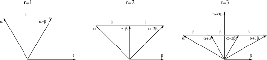
Figure 1: Short-root strings through a long root

It is not hard to see that the subset of roots belonging to any plane spanned by a short root $\beta$ and its string $(\alpha,\alpha{+}\beta,\alpha{+}2\beta,\ldots,\alpha{+}r\beta)$ through a long root $\alpha$ makes the double sum in the left equation of (4.5) already vanish. Since the full double sum decomposes into contributions of such planes, we get a prepotential solution

$$F(t) \ =\ -{\textstyle\frac{1}{2}}\,\Bigl{(}f_{\textrm{L}}\!\!\sum_{\alpha\in\smash{\Phi^{+}_{\textrm{L}}}}\ +\ f_{\textrm{S}}\!\!\sum_{\alpha\in\smash{\Phi^{+}_{\textrm{S}}}}\Bigr{)}\,\alpha(x)^{2}\,\ln|\alpha(x)|$$ (5.5)

$$\ =\ -{\textstyle\frac{1}{2h^{\vee}}}\sum_{\alpha\in\smash{\Phi^{+}}}\alpha(x)^{2}\,\ln|\alpha(x)|\ -\ {\textstyle\frac{t}{2}}\,\Bigl{[}({\textstyle\frac{h\ }{h^{\vee}}}{-}1)\!\!\sum_{\alpha\in\smash{\Phi^{+}_{\textrm{L}}}}-\,(r{-}{\textstyle\frac{h\ }{h^{\vee}}})\!\!\sum_{\alpha\in\smash{\Phi^{+}_{\textrm{S}}}}\Bigr{]}\,\alpha(x)^{2}\,\ln|\alpha(x)|$$

which is unique only for simply-laced Lie algebras. Note that $|f_{\textrm{L}}|$ and $|f_{\textrm{S}}|$ may be absorbed into a rescaling of $\alpha$ but their signs cannot, and so the non-simply-laced solution generalizes the $t{=}0$ one found before [5, 6] by adding to it a concrete $F_{\textrm{hom}}$.

Let us give two examples, with $n{+}1$ and 3 particles, respectively:

$$A_{n}\oplus A_{1}: \{\alpha(x)\}\ =\ \bigl{\{}\ x^{i}{-}x^{j}\ ,\ \textstyle{\sum_{i}}x^{i}\quad\big{|}\quad 1\leq i<j\leq n{+}1\ \bigr{\}}\qquad{\textrm{and}}\qquad f_{\alpha}\ =\ {\textstyle\frac{1}{n+1}}\ ,$$ (5.6)

$$G_{2}\oplus A_{1}: \{\alpha(x)\}\ =\ \bigl{\{}\ {\textstyle\frac{1}{\sqrt{3}}}(x^{i}{+}x^{j}{-}2x^{k})\ ,\ {\textstyle\frac{1}{\sqrt{3}}}(x^{i}{-}x^{j})\ ,\ x^{1}{+}x^{2}{+}x^{3}\quad\big{|}\quad(i,j,k)\quad\textrm{cyclic}\ \bigr{\}}$$ (5.7)

$$\textrm{and}\qquad f_{\textrm{L}}\ =\ {\textstyle\frac{1}{4}}+{\textstyle\frac{1}{2}}t\ ,\quad f_{\textrm{S}}\ =\ {\textstyle\frac{1}{4}}-{\textstyle\frac{3}{2}}t\ ,\quad f_{\textrm{com}}\ =\ {\textstyle\frac{1}{3}}\ .$$

The Weyl groups of the simple Lie algebras can be extended by the non-crystallographic Coxeter groups $H_{4}$ (60 positive roots), $H_{3}$ (15 positive roots) and $I_{2}(p)$ ($p$ positive roots), which also clear the WDVV equation [6]. The dihedral groups $I_{2}(p)$ with $f_{\alpha}={\textstyle\frac{1}{p}}$ cover all rank-two root systems, including $A_{1}{\oplus}A_{1}$, $A_{2}$, $BC_{2}$ and $G_{2}$ for $p=2,3,4$ and $6$, respectively, upon rescaling of $\alpha$.

Figure 2: Root systems of the dihedral groups $I_{2}(p)$ for $p=2,3,4,5,6$.

6 $U{=}0$ solutions: deformed root systems

The Lie-algebra root systems are only the tip of an iceberg of WDVV solutions. It has been shown [7, 9] that certain deformations of them retain the WDVV property. Let us rephrase some examples in our terminology.

The three positive roots of $A_{2}$ may be rearranged as the edges of an equilateral triangle. Consider now a deformation of this triangle, keeping the incidence relation  $\alpha+\beta-\gamma=0$. The homogeneity condition (4.2) (and therefore also the WDVV equation) is easily solved by  $f_{\alpha}\ =\ \frac{|\beta\cdot\gamma|}{4\,A^{2}}$  and cyclic permutations, where $A$ denotes the area of the triangle.

If we try the same idea on the $A_{3}$ system, we obtain the six edges of a regular tetrahedron and deform to encounter the five-dimensional moduli space of tetrahedral shapes (modulo scale).

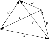
Figure 3: Tetrahedral configuration of covectors

Again, the homogeneity condition (4.2) has a unique solution $f_{\alpha}$, but now the WDVV equation enforces the three conditions

$$\alpha\cdot\alpha^{\prime}=0\ ,\quad\beta\cdot\beta^{\prime}=0\ ,\quad\gamma\cdot\gamma^{\prime}=0$$ (6.1)

on the skew edge pairs. These relations restrict the above moduli space to the three-dimensional subspace of orthocentric tetrahedra (modulo scale), with

$$f_{\alpha}=\frac{|\beta{\cdot}\gamma\ \beta^{\prime}{\cdot}\gamma^{\prime}|}{36\,V^{2}}\qquad{\textrm{and}}\qquad f_{\alpha^{\prime}}=\frac{|\beta{\cdot}\gamma^{\prime}\ \beta^{\prime}{\cdot}\gamma|}{36\,V^{2}}\qquad{\textrm{and}}\qquad\textrm{cyclic}\ ,$$ (6.2)

where $V$ is the volume. Alternatively, we may implement the conditions (6.1) by picking three non-coplanar covectors, say $\alpha^{\prime}$, $\beta^{\prime}$ and $\gamma^{\prime}$, scaling them such that

$$\alpha^{\prime}\cdot\beta^{\prime}\ =\ \beta^{\prime}\cdot\gamma^{\prime}\ =\ \gamma^{\prime}\cdot\alpha^{\prime}\ =\ 1$$ (6.3)

and employing the three-dimensional vector product in fixing the remaining three covectors via

$$\alpha\ =\ \alpha^{\prime}\times(\beta^{\prime}\times\gamma^{\prime})\ =\ \beta^{\prime}-\gamma^{\prime}\ ,\quad\beta\ =\ \beta^{\prime}\times(\gamma^{\prime}\times\alpha^{\prime})\ =\ \gamma^{\prime}-\alpha^{\prime}\ ,\quad\gamma\ =\ \gamma^{\prime}\times(\alpha^{\prime}\times\beta^{\prime})\ =\ \alpha^{\prime}-\beta^{\prime}\ .$$ (6.4)

With these data one gets  $6\,V=\alpha^{\prime}{\cdot}(\beta^{\prime}{\times}\gamma^{\prime})$  as well as

$$f_{\alpha}=\frac{\alpha^{\prime}{\cdot}\alpha^{\prime}{-}1}{36\,V^{2}}\qquad{\textrm{and}}\qquad f_{\alpha^{\prime}}=\frac{(\beta^{\prime}{\cdot}\beta^{\prime}{-}1)(\gamma^{\prime}{\cdot}\gamma^{\prime}{-}1)}{36\,V^{2}}\qquad{\textrm{and}}\qquad\textrm{cyclic}\ .$$ (6.5)

In fact, this strategy generalizes to orthocentric $n$-simplices as $n$-parametric deformations of the regular $n$-simplex generated by the ${\textstyle\frac{1}{2}}n(n{+}1)$ positive roots of $A_{n}$, with

$$f_{\alpha}\ =\ \frac{|\beta{\cdot}\gamma\ \beta^{\prime}{\cdot}\gamma^{\prime}\ \beta^{\prime\prime}{\cdot}\gamma^{\prime\prime}\ \cdots\ \beta^{(n-2)}{\cdot}\gamma^{(n-2)}|}{(n!\ V)^{2}}\quad\textrm{etc.}\ .$$ (6.6)

The orthocentricity derives from the WDVV equation by a the following dimensional reduction argument. Take  $\hat{n}_{i}x^{i}\to\infty$  for some fixed covector $\hat{n}$. Then, any factor $\frac{1}{\alpha(x)}$ in the WDVV equation (4.5) vanishes unless  $\alpha{\cdot}\hat{n}=0$, which amounts to a reduction of the covector set $\{\alpha\}$ to its intersection with the hyperplane orthogonal to $\hat{n}$. This process may be iterated until only covectors laying in a plane $\alpha{\wedge}\beta$ spanned by two covectors $\alpha$ and $\beta$ survive. This situation admits two possibilities: either the $\alpha$ and $\beta$ are concurrent, in which case another covector $\alpha{+}\beta$ or $\alpha{-}\beta$ completes a triangle satisfying the WDVV equation, or else $\alpha$ and $\beta$ are skew, in which case there is no further covector in their plane and WDVV demands orthogonality.

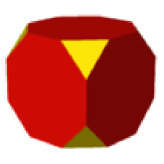
Figure 4: Truncated cube

The $B_{3}$ root system provides another example. Four copies of the 3 short and 6 long positive roots can be assembled into the edge set of a truncated cube. We deform this polyhedron to

$$\bigl{\{}\alpha(x)\bigr{\}}\ =\ \bigr{\{}d_{1}x^{1}\ ,\ d_{2}x^{2}\ ,\ d_{3}x^{3}\ ;\ c_{3}(c_{2}x^{1}{\pm}c_{1}x^{2})\ ,\ c_{1}(c_{3}x^{2}{\pm}c_{2}x^{3})\ ,\ c_{2}(c_{1}x^{3}{\pm}c_{3}x^{1})\bigr{\}}$$ (6.7)

with $c_{i},d_{i}\in\mathbb{R}$, retaining the ‘incidence relations’ of a truncated cuboid. For  $c^{2}:=c_{0}^{2}+c_{1}^{2}+c_{2}^{2}+c_{3}^{2}$  and

$$\bigl{\{}f_{\alpha}\bigr{\}}\ =\ \Bigl{\{}{\textstyle\frac{c_{0}^{2}+c_{1}^{2}-c_{2}^{2}-c_{3}^{2}}{c^{2}\ d_{1}^{2}}}\ ,\ {\textstyle\frac{c_{0}^{2}-c_{1}^{2}+c_{2}^{2}-c_{3}^{2}}{c^{2}\ d_{1}^{2}}}\ ,\ {\textstyle\frac{c_{0}^{2}-c_{1}^{2}-c_{2}^{2}+c_{3}^{2}}{c^{2}\ d_{1}^{2}}}\ ;\ {\textstyle\frac{1}{c^{2}\,c_{3}^{2}}}\ ,\ {\textstyle\frac{1}{c^{2}\,c_{1}^{2}}}\ ,\ {\textstyle\frac{1}{c^{2}\,c_{2}^{2}}}\Bigr{\}}$$ (6.8)

we satisfy the homogeneity condition (4.2), i.e. $\sum_{\alpha}f_{\alpha}\,\alpha{\otimes}\alpha=\mathbbm{1}$. The relevant combinations $\sqrt{f_{\alpha}}\,\alpha$ depend only on the three ratios $c_{i}/c_{0}$. The rigid $B_{3}$ root system with (5.4) occurs for  $c_{1}=c_{2}=c_{3}=1$  and  $c_{0}^{2}=\frac{2-3t}{1+t}$. The case of $C_{3}$ is very similar.

Finally, let us present an example based on weights rather than roots, namely a deformation of the $B_{3}$ representation $\underline{7}\oplus\underline{8}$, i.e. the vector plus spinor weights. For the 3 positive ‘vector’ and 4 positive ‘spinor’ covectors we take

$$\alpha(x)=d_{1}x^{1}\ ,\quad\beta(x)=d_{2}x^{2}\ ,\quad\gamma(x)=d_{3}x^{3}\ ;\quad{\textstyle\frac{\alpha{+}\beta{+}\gamma}{2}}\ ,\quad{\textstyle\frac{\alpha{-}\beta{-}\gamma}{2}}\ ,\quad{\textstyle\frac{-\alpha{+}\beta{-}\gamma}{2}}\ ,\quad{\textstyle\frac{-\alpha{-}\beta{+}\gamma}{2}}$$ (6.9)

with $d_{i}\in\mathbb{R}$, keeping the relations between vector and spinor weights. For  $d^{2}:=d_{1}^{2}+d_{2}^{2}+d_{3}^{2}$  and

$$f_{\alpha}={\textstyle\frac{-d_{1}^{2}+d_{2}^{2}+d_{3}^{2}}{d^{2}\,d_{1}^{2}}}\ ,\quad f_{\beta}={\textstyle\frac{d_{1}^{2}-d_{2}^{2}+d_{3}^{2}}{d^{2}\,d_{2}^{2}}}\ ,\quad f_{\gamma}={\textstyle\frac{d_{1}^{2}+d_{2}^{2}-d_{3}^{2}}{d^{2}\,d_{3}^{2}}}\quad\textrm{and}\quad f_{\textrm{spinor}}={\textstyle\frac{2}{d^{2}}}$$ (6.10)

we obey (4.2) and achieve a two-parameter deformation of the original weight system at  $c_{1}=c_{2}=c_{3}$. The corresponding polyhedron, whose edges are built from 4 copies of the vector and 6 copies of the spinor weights, is a (inhomogeneously scaled) rhombic dodecahedron with the faces dissected into triangles.

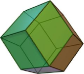
Figure 5: Rhombic dodecahedron

It is important to realize that all examples fulfil the WDVV equation, because the above dimensional reduction argument applies. The crucial properties are the mutual orthogonality of non-concurrent non-parallel edges as well as the incidence relations, which ‘sew’ the triangles together into a polyhedron. Yet, these properties are only necessary but not sufficient. Finally we remark that all our examples are part of a larger moduli space of $n{=}3$ families of WDVV solutions [7, 9].

7 $U{\neq}0$ solutions: no-go ‘theorem’ for $n{>}2$

Recall that, for turning on

$$U\ =\ -\sum_{\alpha}g_{\alpha}\,\ln|\alpha(x)|\qquad\textrm{with}\qquad\sum_{\alpha}g_{\alpha}\ =\ C$$ (7.1)

in a given $F$ background determined by $\{\alpha,f_{\alpha}\}$, we need to solve the flatness condition (4.6). In principle, we may modify (4.6) by adding a homogeneous term $U_{\textrm{hom}}$ to the prepotential above, but let us postpone this option for the time being. Then, matching the coefficients of the double poles in (4.6) requires that

$$\textrm{either}\qquad g_{\beta}=0\qquad\textrm{or else}\qquad\beta{\cdot}\beta\ f_{\beta}=1\qquad\textrm{for each covector $\beta$}\ .$$ (7.2)

In the undeformed irreducible root-system solutions, the Weyl group identifies the $f_{\alpha}$ and $g_{\alpha}$ coefficients for all roots of the same length. Hence, besides the $f_{\textrm{L}}$ and $f_{\textrm{S}}$ values in (5.4) we have couplings $g_{\textrm{L}}$ and $g_{\textrm{S}}$ for a number $p_{\textrm{L}}$ and $p_{\textrm{S}}$ of long and short positive roots, respectively. This simplifies the trace of (5.3) to

$$n\ =\ \sum_{\alpha}\alpha{\cdot}\alpha\,f_{\alpha}\ =\ 2f_{\textrm{L}}\,p_{\textrm{L}}\ +\ {\textstyle\frac{2}{r}}f_{\textrm{S}}\,p_{\textrm{S}}\qquad\longrightarrow\qquad p_{\textrm{L}}+p_{\textrm{S}}\ =\ n\qquad\textrm{if}\quad g_{\textrm{L}},g_{\textrm{S}}\neq 0\ .$$ (7.3)

Since the total number $p_{\textrm{L}}+p_{\textrm{S}}$ of positive roots always exceeds $n$ (except for $A_{1}^{\oplus n}$), we are forced to put either $g_{\textrm{S}}=0$ or $g_{\textrm{L}}=0$. Therefore, all simply-laced root systems are ruled out! For the $r{>}1$ root systems, we get

either $$g_{\textrm{S}}=0\ ,\quad g_{\textrm{L}}=g\qquad\buildrel(\ref{UF3})(\ref{rootsumrule})\over{\longrightarrow}\qquad f_{\textrm{S}}={\textstyle\frac{r}{2}}{\textstyle\frac{n-p_{\textrm{L}}}{p_{\textrm{S}}}}\leq 0\ ,\quad f_{\textrm{L}}={\textstyle\frac{1}{2}}$$ (7.4)

or $$g_{\textrm{S}}=g\ ,\quad g_{\textrm{L}}=0\qquad\buildrel(\ref{UF3})(\ref{rootsumrule})\over{\longrightarrow}\qquad f_{\textrm{S}}={\textstyle\frac{r}{2}}\ ,\quad f_{\textrm{L}}={\textstyle\frac{1}{2}}{\textstyle\frac{n-p_{\textrm{S}}}{p_{\textrm{L}}}}\leq 0\ .$$ (7.5)

We see that in the non-simply-laced one-parameter family (5.4) there is always one member which obeys (7.4) or (7.5). For it, we must still check the remainder of (4.6),

$$\sum_{\alpha\neq\beta}g_{\alpha}f_{\beta}\,\frac{\alpha{\cdot}\beta}{\alpha(x)\ \beta(x)}\ \beta\otimes\beta\ =\ 0\ .$$ (7.6)

Even though its trace is alway satisfied, the traceless part is violated for any nontrivial root system with the data (7.4) or (7.5). Hence, there do not exist $U$ solutions of the standard form (7.1) for any Coxeter root system. Perhaps this no-go result may be overcome by adding suitable $U_{\textrm{hom}}$ contributions. Certainly it can be avoided for $n{=}2$ because in this case (4.4) may be relaxed (see below). Finally, we have not yet studied the flatness conditions for the deformed root systems of the previous section.

8 $U{\neq}0$ solutions: dihedral solutions for $n{=}2$

As mentioned before, the case of three particles with translation invariance, i.e. $n{=}2$, is special for the absence of the WDVV equation. In fact, it is easy to see that any set $\{\alpha\}$ of covectors can be made to obey the left condition in (4.2) with suitably chosen $f_{\alpha}$. To study concrete examples, we look at the most symmetric cases, namely the dihedral root systems mentioned earlier.

It is crucial that we take advantage of the freedom at $n{=}2$ to add ‘radial terms’ in our ansatz:

$$F\!\! = \!\!-{\textstyle\frac{1}{2}}\sum_{\alpha}f_{\alpha}\ \alpha(x)^{2}\ln|\alpha(x)|-{\textstyle\frac{1}{2}}f_{R}\,R^{2}\ln R\quad\longrightarrow\quad\sum_{\alpha}f_{\alpha}\,\alpha{\otimes}\alpha\ =\ (1{-}f_{R})\,\mathbbm{1}\ ,$$ (8.1)

$$U\!\! = \!\!-\sum_{\alpha}g_{\alpha}\,\ln|\alpha(x)|-g_{R}\,\ln R\qquad\qquad\qquad\longrightarrow\quad\sum_{\alpha}g_{\alpha}\ =\ C{-}g_{R}\ .$$ (8.2)

The flatness condition then reduces to (7.2) and the trace of (7.6) plus the relation  $g_{R}+(C{-}g_{R})f_{R}=0$. It is obeyed for the $I_{2}(p)$ system if  $(g_{\textrm{even}},g_{\textrm{odd}}){=:}(g_{\textrm{S}},g_{\textrm{L}})$  when $p$ is even and if  $g_{\alpha}{=:}g\ \forall\alpha$  when $p$ is odd. Turning on $g$ couplings for all covectors fixes $\alpha{\cdot}\alpha\,f_{\alpha}=1$, and so we obtain

$$p=2\,(1{-}f_{R})\qquad\longrightarrow\qquad g_{R}={\textstyle\frac{p-2}{p}}\,C\qquad\longrightarrow\qquad{\textstyle\frac{2}{p}}C=\sum_{\alpha}g_{\alpha}=\Bigl{\{}\begin{smallmatrix}{\textstyle\frac{p}{2}}(g_{\textrm{S}}{+}g_{\textrm{L}})\ &\textrm{for $p$ even}\\ p\,g&\textrm{for $p$ odd}\end{smallmatrix}\ \ .$$ (8.3)

In order to ease the interpretation as three-particle systems, we embed the relative-motion configuration space $\mathbb{R}^{2}$ into $\mathbb{R}^{3}\ni(x^{1},x^{2},x^{3})$  and rotate such that  $\alpha_{\textrm{com}}=(1,1,1)$. For identical particles we require invariance under permutations  $(x^{1},x^{2},x^{3})\to(x^{\pi_{1}},x^{\pi_{2}},x^{\pi_{3}})$  of the full three-body coordinates. This limits $p$ to multiples of 3. The ‘radial coordinate’ then becomes

$$R^{2}\ =\ {\textstyle\frac{1}{3}}\bigl{\{}(x^{12})^{2}+(x^{23})^{2}+(x^{31})^{2}\bigr{\}}\ =\ {\textstyle\frac{2}{3}}\bigl{\{}(x^{1})^{2}+(x^{2})^{2}+(x^{3})^{2}-x^{1}x^{2}-x^{2}x^{3}-x^{3}x^{1}\bigr{\}}\ .$$ (8.4)

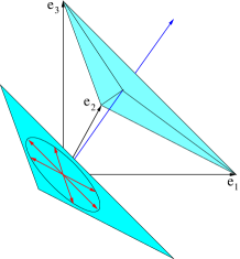
Figure 6: Embedding of $A_{2}$ roots into $\mathbb{R}^{3}$

9 Examples

For illustration we explicitly display the $I_{2}(p)$ solutions based on (8.1) and (8.2) for the first few values of $p$.

$\underline{p{=}2}\ :\quad A_{1}{\oplus}A_{1}$ model $f_{R}{=}0\,,\quad g_{R}{=}0\quad\longrightarrow\quad g_{\textrm{S}}{+}g_{\textrm{L}}{=}C$

$$\frac{\alpha(x)}{\sqrt{\alpha{\cdot}\alpha}}\ \in\ \Bigl{\{}{\textstyle\frac{1}{\sqrt{2}}}(x^{1}{-}x^{2})\,,\,{\textstyle\frac{1}{\sqrt{6}}}(x^{1}{+}x^{2}{-}2x^{3})\Bigr{\}}\qquad\qquad\qquad\qquad\qquad\qquad\qquad\ \$$

$$V_{B}\ =\ \frac{g_{\textrm{S}}^{2}{+}{\textstyle\frac{{\hbar}^{2}}{4}}}{(x^{1}{-}x^{2})^{2}}\ +\ \frac{3\,(g_{\textrm{L}}^{2}{+}{\textstyle\frac{{\hbar}^{2}}{4}})}{(x^{1}{+}x^{2}{-}2x^{3})^{2}}\qquad\qquad\qquad\qquad\qquad\qquad\qquad\qquad$$

$\underline{p{=}3}\ :\quad A_{2}$ model $f_{R}{=}{-}{\textstyle\frac{1}{2}}\,,\quad g_{R}{=}{\textstyle\frac{1}{3}}C\quad\longrightarrow\quad g{=}{\textstyle\frac{2}{9}}C$

$$\frac{\alpha(x)}{\sqrt{\alpha{\cdot}\alpha}}\ \in\ \Bigl{\{}{\textstyle\frac{1}{\sqrt{2}}}(x^{1}{-}x^{2})\,,\,{\textstyle\frac{1}{\sqrt{2}}}(x^{1}{-}x^{3})\,,\,{\textstyle\frac{1}{\sqrt{2}}}(x^{2}{-}x^{3})\Bigr{\}}\qquad\qquad\qquad\qquad\qquad\quad\ \$$

$$V_{B}\ =\ \bigl{(}g^{2}{+}{\textstyle\frac{{\hbar}^{2}}{4}}\bigr{)}\,\biggl{(}\frac{1}{(x^{1}{-}x^{2})^{2}}+\frac{1}{(x^{2}{-}x^{3})^{2}}+\frac{1}{(x^{3}{-}x^{1})^{2}}\biggr{)}\ +\ {\textstyle\frac{5}{8}}\,\bigl{(}9g^{2}{-}{\hbar}^{2}\bigr{)}\,\frac{1}{R^{2}}$$

$\underline{p{=}4}\ :\quad BC_{2}$ model $f_{R}{=}{-}1\,,\quad g_{R}{=}{\textstyle\frac{1}{2}}C\quad\longrightarrow\quad g_{\textrm{S}}{+}g_{\textrm{L}}{=}{\textstyle\frac{1}{4}}C$

$$\frac{\alpha(x)}{\sqrt{\alpha{\cdot}\alpha}}\in\Bigl{\{}{\textstyle\frac{x^{1}{-}x^{2}}{\sqrt{2}}}\,,\,{\textstyle\frac{x^{1}{+}x^{2}{-}2x^{3}}{\sqrt{6}}}\,,\,{\textstyle\frac{\tau x^{1}{-}\bar{\tau}x^{2}{-}x^{3}}{\sqrt{3}}}\,,\,{\textstyle\frac{-\bar{\tau}x^{1}{+}\tau x^{2}{-}x^{3}}{\sqrt{3}}}\Bigr{\}}\quad\textrm{with}\quad\biggl{\{}\begin{smallmatrix}\tau={\textstyle\frac{1}{2}}(\sqrt{3}{+}1)\\[4.0pt] \bar{\tau}={\textstyle\frac{1}{2}}(\sqrt{3}{-}1)\end{smallmatrix}$$

$$\qquad V_{B}\ =\ \frac{g_{\textrm{S}}^{2}{+}{\textstyle\frac{{\hbar}^{2}}{4}}}{(x^{1}{-}x^{2})^{2}}+\frac{3\,(g_{\textrm{S}}^{2}{+}{\textstyle\frac{{\hbar}^{2}}{4}})}{(x^{1}{+}x^{2}{-}2x^{3})^{2}}+\frac{\frac{3}{2}\,(g_{\textrm{L}}^{2}{+}\frac{{\hbar}^{2}}{4})}{(\tau x^{1}{-}\bar{\tau}x^{2}{-}x^{3})^{2}}+\frac{\frac{3}{2}\,(g_{\textrm{L}}^{2}{+}\frac{{\hbar}^{2}}{4})}{({-}\bar{\tau}x^{1}{+}\tau x^{2}{-}x^{3})^{2}}+\frac{6(g_{\textrm{S}}{+}g_{\textrm{L}})^{2}{-}\frac{3}{2}{\hbar}^{2}}{R^{2}}$$

$\underline{p{=}6}\ :\quad G_{2}$ model $f_{R}{=}{-}2\,,\quad g_{R}{=}{\textstyle\frac{2}{3}}C\quad\longrightarrow\quad g_{\textrm{S}}{+}g_{\textrm{L}}{=}{\textstyle\frac{1}{9}}C$

$$\frac{\alpha(x)}{\sqrt{\alpha{\cdot}\alpha}}\ \ \in\ \ \Bigl{\{}{\textstyle\frac{x^{1}{-}x^{2}}{\sqrt{2}}}\,,\,{\textstyle\frac{x^{1}{-}x^{3}}{\sqrt{2}}}\,,\,{\textstyle\frac{x^{2}{-}x^{3}}{\sqrt{2}}}\,,\,{\textstyle\frac{2x^{1}{-}x^{2}{-}x^{3}}{\sqrt{6}}}\,,\,{\textstyle\frac{x^{1}{+}x^{2}{-}2x^{3}}{\sqrt{6}}}\,,\,{\textstyle\frac{-x^{1}{+}2x^{2}{-}x^{3}}{\sqrt{6}}}\Bigr{\}}\qquad\quad$$

$$V_{B}\ =\ \frac{g_{\textrm{S}}^{2}{+}{\textstyle\frac{{\hbar}^{2}}{4}}}{(x^{1}{-}x^{2})^{2}}\ +\ \frac{3\,(g_{\textrm{L}}^{2}{+}{\textstyle\frac{{\hbar}^{2}}{4}})}{(x^{1}{+}x^{2}{-}2x^{3})^{2}}\ +\ \textrm{cyclic}\ +\ \frac{36(g_{\textrm{S}}{+}g_{\textrm{L}})^{2}{-}4{\hbar}^{2}}{R^{2}}\qquad\quad$$

$\underline{p{=}12}\ :\quad I_{2}(12)$ model $f_{R}{=}{-}5\,,\quad g_{R}{=}{\textstyle\frac{5}{6}}C\quad\longrightarrow\quad g_{\textrm{S}}{+}g_{\textrm{L}}{=}{\textstyle\frac{1}{36}}C$

$$\qquad\quad\ \begin{aligned} \frac{\alpha(x)}{\sqrt{\alpha{\cdot}\alpha}}\ \ \in\ \ \Bigl{\{}{\textstyle\frac{x^{1}{-}x^{2}}{\sqrt{2}}}\,,\,{\textstyle\frac{x^{1}{-}x^{3}}{\sqrt{2}}}\,,\,{\textstyle\frac{x^{2}{-}x^{3}}{\sqrt{2}}}\,,\,{\textstyle\frac{2x^{1}{-}x^{2}{-}x^{3}}{\sqrt{6}}}\,,\,{\textstyle\frac{x^{1}{+}x^{2}{-}2x^{3}}{\sqrt{6}}}\,,\,{\textstyle\frac{-x^{1}{+}2x^{2}{-}x^{3}}{\sqrt{6}}}\,,\qquad\qquad\qquad\quad\!\\[4.0pt] {\textstyle\frac{\tau x^{1}{-}x^{2}{-}\bar{\tau}x^{3}}{\sqrt{3}}}\,,\,{\textstyle\frac{\tau x^{1}{-}\bar{\tau}x^{2}{-}x^{3}}{\sqrt{3}}}\,,\,{\textstyle\frac{x^{1}{+}\bar{\tau}x^{2}{-}\tau x^{3}}{\sqrt{3}}}\,,\,{\textstyle\frac{\bar{\tau}x^{1}{+}x^{2}{-}\tau x^{3}}{\sqrt{3}}}\,,\,{\textstyle\frac{-\bar{\tau}x^{1}{+}\tau x^{2}{-}x^{3}}{\sqrt{3}}}\,,\,{\textstyle\frac{-x^{1}{+}\tau x^{2}{-}\bar{\tau}x^{3}}{\sqrt{3}}}\Bigr{\}}\end{aligned}$$

$$\qquad\qquad\quad\begin{aligned} V_{B}&\ =\ \frac{g_{\textrm{S}}^{2}{+}{\textstyle\frac{{\hbar}^{2}}{4}}}{(x^{1}{-}x^{2})^{2}}\ +\ \frac{3\,(g_{\textrm{S}}^{2}{+}{\textstyle\frac{{\hbar}^{2}}{4}})}{(x^{1}{+}x^{2}{-}2x^{3})^{2}}\ +\ \frac{\frac{3}{2}\,(g_{\textrm{L}}^{2}{+}{\textstyle\frac{{\hbar}^{2}}{4}})}{(\tau x^{1}{-}x^{2}{-}\bar{\tau}x^{3})^{2}}\ +\ \frac{\frac{3}{2}\,(g_{\textrm{L}}^{2}{+}{\textstyle\frac{{\hbar}^{2}}{4}})}{(\tau x^{1}{-}\bar{\tau}x^{2}{-}x^{3})^{2}}\ +\ \textrm{cyclic}\\[4.0pt] &\qquad+\ \frac{630(g_{\textrm{S}}{+}g_{\textrm{L}})^{2}{-}\frac{35}{2}{\hbar}^{2}}{R^{2}}\end{aligned}$$

Finally, let us investigate the effect of adding to $U$ a homogeneous piece $U_{\text{hom}}$ for obtaining $U_{\textrm{tot}}=U+U_{\text{hom}}$. At $n{=}2$, all we have to solve is the trace of the flatness condition,

$$\partial{\cdot}\partial\,U_{\text{hom}}\ +\ \sum_{\alpha}{f_{\alpha}\,\alpha{\cdot}\alpha}\ {\textstyle\frac{\alpha\cdot\partial}{\alpha(x)}}\,U_{\text{hom}}\ =\ 0\qquad\textrm{besides}\qquad x^{i}\partial_{i}U_{\text{hom}}=0\ .$$ (9.1)

It is convenient to pass to polar coordinates on $\mathbb{R}^{2}$ via  $(x^{1},x^{2})=(R\cos\phi,R\sin\phi)$. In the dihedral class $I_{2}(p)$, the sum over the roots can be performed, and the flatness conditions for $U$ and for $U_{\text{hom}}$ is solved by

$$U(R,\phi) \ =\ -C\,\ln R\ -\ \begin{cases}g\,\ln|\cos(p\phi)|&\textrm{for $p$ odd}\\[4.0pt] g_{\textrm{S}}\ln|\cos({\textstyle\frac{p}{2}}\phi)|+g_{\textrm{L}}\ln|\sin({\textstyle\frac{p}{2}}\phi)|&\textrm{for $p$ even}\end{cases}\ \ ,$$ (9.2)

$$U_{\text{hom}}(\phi) \ =\ {\textstyle\frac{\lambda}{p}}\,\ln|\tan({\textstyle\frac{p}{2}}\phi{+}\delta)|\qquad\qquad\ \ \,\textrm{with}\qquad\delta\ =\ \Bigl{\{}\begin{matrix}{\textstyle\frac{\pi}{4}}&\textrm{for $p$ odd}\\ 0&\textrm{\ for $p$ even}\end{matrix}\ \ \ .$$

After lifting to the full configuration space $\mathbb{R}^{3}$ as in Figure 6, we arrive at

$$\partial_{i}U_{\textrm{tot}}\ =\ -\sum_{\alpha}g_{\alpha}\,\frac{\alpha_{i}}{\alpha(x)}\ -\ {\textstyle\frac{p-2}{p}}\,C\,\frac{x_{i}}{R^{2}}\ +\ \lambda\,\biggl{(}\begin{smallmatrix}x^{2}{-}x^{3}\\ x^{3}{-}x^{1}\\ x^{1}{-}x^{2}\end{smallmatrix}\biggr{)}\,R^{p-2}\,\prod_{\alpha}\bigl{(}\alpha(x)\bigr{)}^{-1}\ .$$ (9.3)

For the $A_{2}$ model as the simplest example, one gets

$$F\ =\ -{\textstyle\frac{1}{4}}\,\bigl{(}(x^{12})^{2}\ln|x^{12}|+(x^{23})^{2}\ln|x^{23}|+(x^{31})^{2}\ln|x^{31}|\bigr{)}\ +\ {\textstyle\frac{1}{4}}\,R^{2}\ln R\ ,$$ (9.4)

$$\vec{\nabla}U_{\textrm{tot}}\ \ =\ \ \bigl{[}x^{12}x^{23}x^{31}\bigr{]}^{-1}\,\biggl{(}\begin{smallmatrix}[\lambda R-g(x^{31}{-}x^{12})]\,x^{23}\\ [\lambda R-g(x^{12}{-}x^{23})]\,x^{31}\\ [\lambda R-g(x^{23}{-}x^{31})]\,x^{12}\end{smallmatrix}\biggr{)}\ -\ {\textstyle\frac{3}{2}}\,g\,R^{-2}\,\biggl{(}\begin{smallmatrix}x^{1}\\ x^{2}\\ x^{3}\end{smallmatrix}\biggr{)}\ ,\qquad\quad$$ (9.5)

$$V_{B}^{\textrm{tot}} \ =\ \bigl{(}g^{2}+{\textstyle\frac{2}{3}}\lambda^{2}+{\textstyle\frac{{\hbar}^{2}}{4}}\bigr{)}\,\Bigl{(}\frac{1}{(x^{12})^{2}}+\frac{1}{(x^{23})^{2}}+\frac{1}{(x^{31})^{2}}\Bigr{)}$$ (9.6)

$$\quad+\ \ {\textstyle\frac{5}{8}}\bigl{(}9g^{2}-{\hbar}^{2}\bigr{)}\,R^{-2}\ +\ \lambda\,g\,R\,\frac{(x^{12}{-}x^{23})(x^{23}{-}x^{31})(x^{31}{-}x^{12})}{(x^{12}\,x^{23}\,x^{31})^{2}}\ ,$$

with  $R^{2}={\textstyle\frac{1}{3}}\bigl{\{}(x^{12})^{2}+(x^{23})^{2}+(x^{31})^{2}\bigr{\}}$. A pure Calogero potential is possible only for  $g=0={\hbar}$.

Acknowledgements

The author is grateful to Anton Galajinsky and Kirill Polovnikov for a very fruitful collaboration. His work is partially supported by the Deutsche Forschungsgemeinschaft.

References

• [1] N. Wyllard, J. Math. Phys. 41 (2000) 2826 [hep-th/9910160].
• [2] S. Bellucci, A. Galajinsky, E. Latini, Phys. Rev. D 71 (2005) 044023 [hep-th/0411232].
• [3] E. Witten, Nucl. Phys. B 340 (1990) 281.
• [4] R. Dijkgraaf, H. Verlinde, E. Verlinde, Nucl. Phys. B 352 (1991) 59.
• [5] R. Martini, P.K.H. Gragert, J. Nonlin. Math. Phys. 6 (1999) 1 [hep-th/9901166].
• [6] A.P. Veselov, Phys. Lett. A 261 (1999) 297 [hep-th/9902142].
• [7] O.A. Chalykh, A.P. Veselov, Phys. Lett. A 285 (2001) 339 [math-ph/0105003].
• [8] A. Galajinsky, O. Lechtenfeld, K. Polovnikov, JHEP 0711 (2007) 008 [arXiv:0708.1075 [hep-th]].
• [9] M.V. Feigin, A.P. Veselov, Adv. Math. 212 (2007) 143 [math-ph/0512095];
“On the geometry of $\vee$-systems”, arXiv:0710.5729 [math-ph].
• [10] A. Galajinsky, O. Lechtenfeld, K. Polovnikov,
“N=4 mechanics, WDVV equations and roots,” arXiv:0802.4386 [hep-th].