Multi-Satellite Observations of Cygnus X-1
to Study the Focused Wind and Absorption Dips

Abstract:

High-mass X-ray binary systems are powered by the stellar wind of their donor stars. The X-ray state of Cygnus X-1 is correlated with the properties of the wind which defines the environment of mass accretion. Chandra-HETGS observations close to orbital phase 0 allow for an analysis of the photoionzed stellar wind at high resolution, but because of the strong variability due to soft X-ray absorption dips, simultaneous multi-satellite observations are required to track and understand the continuum, too. Besides an earlier joint Chandra and RXTE observation, we present first results from a recent campaign which represents the best broad-band spectrum of Cyg X-1 ever achieved: On 2008 April 18/19 we observed this source with XMM-Newton, Chandra, Suzaku, RXTE, INTEGRAL, Swift, and AGILE in X- and $\gamma$-rays, as well as with VLA in the radio. After superior conjunction of the black hole, we detect soft X-ray absorption dips likely due to clumps in the focused wind covering $\geq 95\,\%$ of the X-ray source, with column densities likely to be of several $10^{23}\,$cm^-2, which also affect photon energies above 20 keV via Compton scattering.

Introduction

One of the currently still puzzling issues in our understanding of microquasars is the existence of the different states (low/hard, high/soft, very high/steep power-law, …), which distinguish themselves by the soft X-ray luminosity, the X-ray spectrum, the timing properties, and also the nature of the jet and its radio spectrum. One assumes that these states with their in many ways different properties correspond to different configurations of the accretion flow which cause different channels or efficiencies of energy dissipation. For a high-mass X-ray binary system, the global framework of mass accretion onto the black hole is defined by the powering wind of the donor star. One possibility is that changes in the wind properties (like density, velocity, ionization parameter, …) might finally trigger state transitions.

This contribution focuses on the wind of the well-known persistently bright X-ray source Cygnus X-1. Its companion star HDE 226868, a $\sim$18$\,M_{\odot}$ O9.7 type supergiant [11], fills 97 % of its Roche lobe [6]. The stellar wind is therefore strongly focused due to tidal interactions [5, 7]. The detailed structure of this wind defines the environment of mass accretion onto the black hole on the largest scale. At a luminosity of $L_{0.5-250\,\mathrm{keV}}=3\times 10^{37}\,$erg s^-1 (which is obtained already in the low/hard state [9]), the X-ray source produces a considerable feedback on the wind by photoionization [2], which can create a complex wind structure within the binary system. The parameters inferred from the H$\alpha$ emission line are (anti-)correlated with the X-ray flux: in the low/hard state, the wind is probably denser and therefore less strongly ionized, which allows for a more efficient wind acceleration and thus a lower accretion rate onto the black hole [8].

We have obtained multi-satellite observations of Cyg X-1 in the hard state close to superior conjunction of the black hole, i.e., at phase $\phi_{\mathrm{orb}}\approx 0$ in the 5.6 day binary orbit [3, 8], which are ideal to investigate the wind: at the low inclination $i\approx 35^{\circ}$ [11], no eclipses of Cyg X-1 by its companion star can be observed. Nevertheless, absorption dips, which are likely related to the focused stream covering the X-ray source, are often detected close to $\phi_{\mathrm{orb}}=0$ [1].

1 The Chandra and RXTE observation of 2003 April

1.1 Advantages of a multi-satellite observation

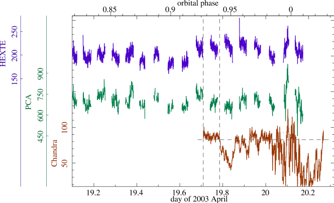
Figure 1: Light curves of Cyg X-1 during the simultaneous Chandra / RXTE observation of 2003 April. Top: RXTE-HEXTE (20–250 keV). Middle: RXTE-PCA (4–20 keV). Bottom: Chandra-HETGS (0.5–12 keV 1^st order events). The dashed lines define the non-dip times.

In the first part of this contribution, we show some of the results from a simultaneous observation of Cyg X-1 performed by Chandra and RXTE in 2003 April shortly before $\phi_{\mathrm{orb}}=0$. (More details are given by Hanke et. al [9, 10].) The light curves shown in Fig. 1 clearly show the advantages of a multi-satellite observation: Due to RXTE’s low Earth orbit, there are data gaps of $\sim$45 minutes length in each RXTE-orbit (lasting $\sim$90 minutes) from passages through the South Atlantic Anomaly (SAA). The high variability which is present on timescales of hours and which is related to the stellar wind could hardly be investigated with the RXTE data alone. The (continuous) soft X-ray light curve taken by Chandra is shaped by absorption dips. Only the joint spectral analysis of the non-dip continuum allows to combine the strength of the different instruments. For example, the PCA spectrum clearly requires an Fe K$\alpha$ emission line at 6.4 keV, but the resolution is not good enough to decide whether it is narrow or relativistically broadened. In the simultaneous Chandra spectrum, a narrow component is detected (see Fig. 2), but its flux is not sufficient to explain the PCA feature, from which we infer the presence of a broad iron line as well. (More details on iron lines in Cyg X-1 are given by M. A. Nowak in his contribution to this volume [16].)

1.2 The non-dip spectrum

The non-dip spectrum can be obtained by filtering for high count rates, see the dashed horizontal line in Fig. 1. The results of this subsection are thoroughly described by Hanke et al. (2008) [9].

The Chandra-HETGS spectrum of the bright source Cyg X-1 shows neutral absorption signatures of the interstellar medium (and probably also source environment). We detect structured absorption edges, namely the Fe L₂ and L₃ edges at 17.2 and 17.5 Å (0.721 and 0.708 keV) – which J. C. Lee describes in detail in her contribution in this volume –, the O K-edge at 22.8 Å (0.544 keV) with the K$\alpha$ resonance absorption line, and the Ne K-edge at 14.3 Å (0.867 keV) with the K$\beta$ resonance absorption line. These complex absorption edges can be modelled with tbnew, an improved version of tbvarabs, which contains those fine structures.

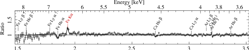
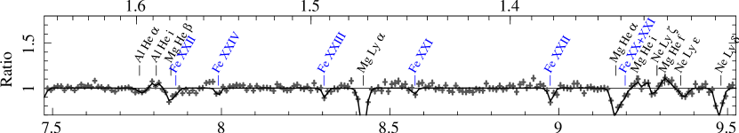
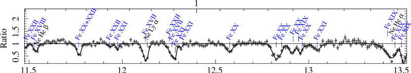
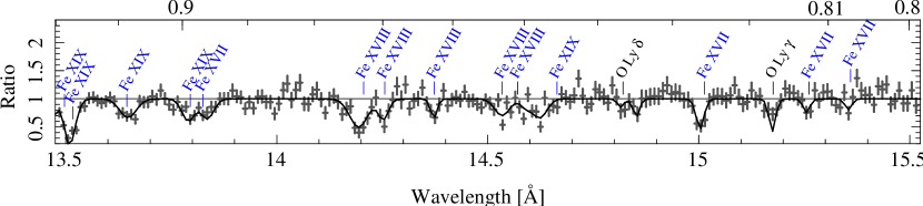
Figure 2: Chandra-HETGS Cyg X-1 non-dip spectrum with identification and fits of absorption lines of H- and He-like ions (Lyman and Helium series; black labels) and Fe L-shell ions (blue labels). Note the narrow and broad Fe K$\alpha$ line (red) at 1.94 Å ($\equiv$6.4 keV, see second $x$- (energy-) axis on top of each panel).

The non-dip spectrum is dominated by absorption lines from the stellar wind of highly ionized ions, namely H- and He-like O, Ne, Na, Mg, Al, Si, S, Ar, Ca, and Fe, as well as many Fe L-shell absorption lines, see Fig. 2. We fit these features with Gaussian absorption lines and infer equivalent widths and Doppler shifts with respect to the rest wavelengths of the identified transitions. In a second approach, we have defined a fit-function (in ISIS [12, 15]) for the whole series of absorption lines of an ion. Theoretical Voigt profiles were used which take into account the oscillator strengths of the strongest transitions. The ion’s column density is a direct fit-parameter of the model, avoiding an explicit curve of growth analysis. The velocity shifts inferred from both methods are rather low, mostly $|v|<200\,$km s^-1.

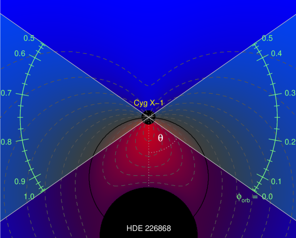
Figure 3: Wind velocity, projected against the black hole. Absorption lines with low velocity $v_{\mathrm{rad}}$ can be observed from the dark purple region close to the black Thales circle of $v_{\mathrm{rad}}=0$, $v_{\mathrm{rad}}>0$ can only be observed from the red region inside this circle, and $v_{\mathrm{rad}}<0$ only from the blue region outside of it. The brighter the red or blue, the higher is $|v_{\mathrm{rad}}(\vec{\boldsymbol{r}})|$. The dashed gray lines are contours of constant $v_{\mathrm{rad}}$ in steps of 200 km s^-1. The highlighted area with the $\phi_{\mathrm{orb}}$ scale shows the region in the orbital plane with $|\cos\vartheta|\leq\sin i$, which equivalently corresponds to all possible lines of sight (for $i=35^{\circ}$).

The latter result can be understood within a simple model for the spherical wind, e.g., a generalized CAK-model [4, 14]:

$$\vec{\boldsymbol{v}}(\vec{\boldsymbol{r}})\;\;=\;\;v(r)\cdot\frac{\vec{\boldsymbol{r}}}{r}\;\quad\quad\mbox{with}\quad v(r)\;\;=\;\;v_{0}\;\;+\;\;(v_{\infty}-v_{0})\cdot\left(1-\frac{R_{\star}}{r}\right)^{\beta}$$ (1)

For the velocity observed in X-ray absorption lines, one has to consider the projection against the black hole, $v_{\mathrm{rad}}(\vec{\boldsymbol{r}})\>=\>\cos\alpha(\vec{\boldsymbol{r}})\cdot v(\vec{\boldsymbol{r}})\>$, where $\alpha(\vec{\boldsymbol{r}})$ is the angle between wind velocity $\vec{\boldsymbol{v}}(\vec{\boldsymbol{r}})$ and the line of sight towards the black hole. Figure 3 shows $v_{\mathrm{rad}}(\vec{\boldsymbol{r}})$ as a colorscale plot. On the circle passing through the center of the star and the black hole, $\alpha=90^{\circ}$ by Thales’ theorem, and thus $v_{\mathrm{rad}}=0$ – independent of the assumed velocity law, as long as it is spherically symmetric.The circle separates (possible) absorbing regions of the wind seen at a redshift (inside) from those seen at a blueshift (outside). The location of absorbers seen at a low velocity is thus well constrained. It is important to realize that this result does not depend on the model for the wind velocity, provided that $\vec{\boldsymbol{v}}(\vec{\boldsymbol{r}})$ points radially away from the star.

Due to the system’s inclination, not every line of sight in the orbital plane can actually be observed: the angle $\vartheta$ between the inclined line of sight $\vec{\boldsymbol{l}}=(\sin i,\;\>0,\;\>\cos i)$ and the binary axis $\vec{\boldsymbol{a}}=\big{(}\cos(2\pi\phi_{\mathrm{orb}}),\;\sin(2\pi\phi_{\mathrm{orb}}),\;0\big{)}$ is given by $\cos\vartheta=\vec{\boldsymbol{l}}\,\circ\,\vec{\boldsymbol{a}}=\sin i\cdot\cos(2\pi\phi_{\mathrm{orb}})$. The range of possible $\vartheta$ values is obviously limited by a low inclination. (For a face-on geometry with $i=0^{\circ}$, there is clearly no orbital variation, i.e. $\vartheta\equiv 90^{\circ}$, while every $0\leq\vartheta\leq 180^{\circ}$ is possible for edge-on systems with $i=90^{\circ}$.) The region with $|\cos\vartheta|\leq\sin i$ is highlighted in Fig. 3 between the crossing solid gray lines. For a spherically symmetrical wind, this region in the orbital plane is equivalent to all lines of sight experienced by an inclined observer. The green labels show the position of these lines of sight for given orbital phases $\phi_{\mathrm{orb}}$, where $\phi_{\mathrm{orb}}$ and $1-\phi_{\mathrm{orb}}$ are identical.

As a result, the observation of low Doppler velocities in absorption lines in front of the X-ray source constrains the location of the absorber – rather independently of the wind model. This location is in good agreement with xstar simulations of the photoionization zone. The number density of H-atoms, $n_{\mathrm{H}}$, is obtained from the velocity profile (Eq. 1) and the continuity equation, $\dot{M}_{\star}\;=\;\mu\,m_{\mathrm{H}}\cdot n_{\mathrm{H}}(r)\cdot 4\pi r^{2}\cdot v(r)$. Here, $\mu=1.4$ is the mean molecular weight per H-atom and $m_{\mathrm{H}}$ is the mass of an H-atom. Inserting the numbers $v_{\infty}=2100\,\mathrm{km\,s}^{-1}$ and $R_{\star}=17\,R_{\odot}$ [11] gives:

$$n_{\mathrm{H}}(r)\;=\;2.2\!\times\!10^{10}\,\mathrm{cm}^{-3}\cdot d(r/R_{\star})\;\;,\;\;\mbox{where}\;\;d(x)\;=\;\frac{x^{-2}}{v_{0}/v_{\infty}\,+\,\left(1-v_{0}/v_{\infty}\right)\cdot\left(1-1/x\right)^{\beta}}$$ (2)

Between the stellar surface and the black hole, $x=r/R_{\star}$ varies between 1 and 2.4 and the average wind density is $n_{\mathrm{H}}\approx 10^{11}\,$cm^-3 for $v_{0}/v_{\infty}=v_{\mathrm{therm}}/v_{\infty}=0.01$ and a reasonable $\beta\approx 1$.

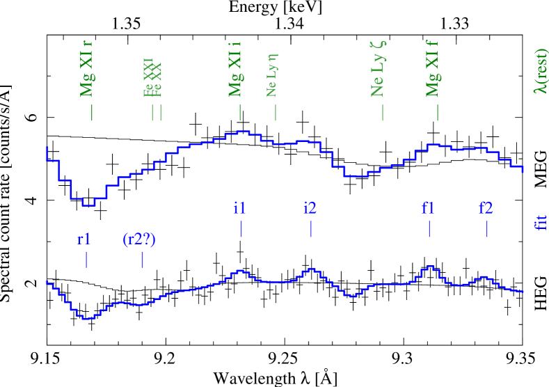
Figure 4: The Mg xi triplet of resonance (r) absorption and intercombination (i) as well as forbidden (f) emission lines is detected with two pairs of i- and f-lines in the non-dip Chandra-HETGS spectra of Cyg X-1. The red-shifted pair stems from an emitting plasma component of higher density and can be identified with the focused wind.

While these previous findings from the non-dip spectrum could be explained by a spherical wind only, there are also signatures of a focused wind: Figure 4 shows the Mg xi triplet of $\rm 1s^{2}\,(^{1}S_{0})\rightarrow 1s2p\,(^{1}P_{1})$ “resonance” (r), $\rm 1s^{2}\,(^{1}S_{0})\leftarrow 1s2p\,(^{3}P_{1,2})$ “intercombination” (i) and $\rm 1s^{2}\,(^{1}S_{0})\leftarrow 1s2s\,(^{3}S_{1})$ “forbidden” (f) transitions. The i- and f-emission lines show up as two components each: one pair is almost at rest – in accord with the r absorption line –, while the other pair is seen at a strong redshift (500–900 km s^-1). The ratio $R=F($f$)/F($i$)$ of the line fluxes is usually used for density diagnostics [17]. However, in the presence of strong UV-radiation fields (such as in the vicinity of HDE 226868), the $R$ ratio is systematically decreased due to photodepletion of the $\rm 1s2s\,(^{3}S_{1})$ level [13]. Therefore, an absolute density analysis would overestimate the density. One can, however, still infer the relative statement that the red-shifted pair of i- and f-lines (with the lower $R$-ratio) stems from a much denser emitting plasma component. Both its velocity and its density indicate that this component can be identified with the focused wind.

1.3 The dip-spectrum

During the dips (Fig. 5a), the soft X-ray spectrum is considerably absorbed. Defining the soft X-ray color as the ratio of the 0.5–1.5 keV and the 1.5–3 keV Chandra count rate, and the hard color as the ratio of 1.5–3 keV and 3–10 keV rate, a color-color diagram (Fig. 5b) shows that neutral photoabsorption alone cannot explain the data. The nose-like shape of the data points can be explained by a partial covering model for the photoelectric absorption:

$$(1-f_{\mathrm{c}})\cdot\mathrm{e}^{-N_{\mathrm{H,1}}^{\mathrm{ISM}}\cdot\sigma_{\mathrm{bf}}(E)}\;+\;f_{\mathrm{c}}\cdot\mathrm{e}^{-N_{\mathrm{H,2}}\cdot\sigma_{\mathrm{bf}}(E)}$$ (3)

We use a constant $N_{\mathrm{H,1}}^{\mathrm{ISM}}=5.4\!\times\!10^{21}\,\mathrm{cm}^{-2}$ and a power-law continuum with photon index $\Gamma=1.73$ as found with RXTE-PCA for the non-dip spectrum [9]. In this model, the strongest dips can be described by an additional absorber with $N_{\mathrm{H,2}}>4\!\times\!10^{23}\,\mathrm{cm}^{-2}$ covering a fraction $f_{\mathrm{c}}$ between 95 % and 98 % of the X-ray source.

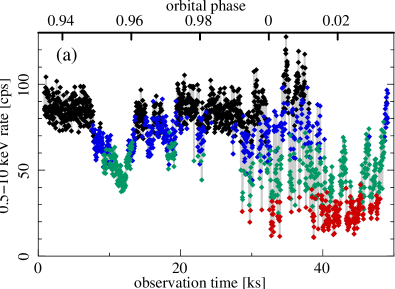
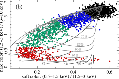
Figure 5: (a): Chandra-HETGS (0.5–10 keV) light curve (see also Fig. 1). (b): Color-color diagram from (0.5–1.5 keV)$:$(1.5–3 keV) and (1.5–3 keV)$:$(3–10 keV) count rate ratios in 25 s intervals, explained by a grid of partial covering models (Eq. 1.3), assuming a power-law continuum ($\Gamma=1.73$). The gray labels indicate the covering fraction $f_{\mathrm{c}}$ in % and the column density $N_{\mathrm{H,2}}$ of the additional absorber in $10^{22}\,$cm^-2.

The high-resolution dip spectra (see, e.g., Fig. 6) show strong absorption lines of lower ionized ions, e.g., resonance K$\alpha$ absorption lines of Si vi–xi between 6.8 and 7.1 Å, which are not detected in the non-dip spectrum at all. This result is consistent with an origin of the dips in colder matter in the focused wind which covers the X-ray source. (More details will be presented in [10].)

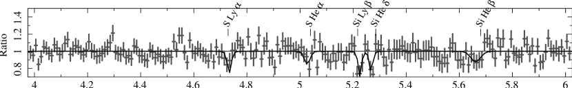
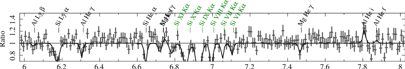
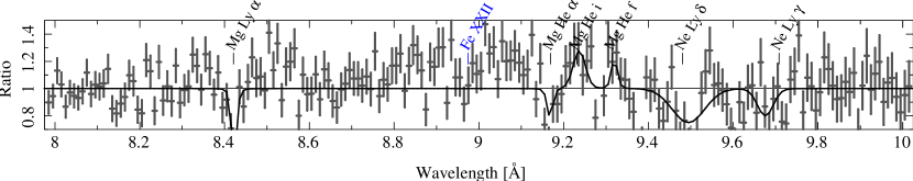
Figure 6: Chandra-HETGS Cyg X-1 spectrum of the first dip ($\phi_{\mathrm{orb}}<0.96$, see Fig. 5a). While the non-dip spectrum (Fig. 2) showed silicon resonance K$\alpha$ absorption lines of only Si xiv and xiii (Si Ly$\alpha$ at 6.18 Å and Si He$\alpha$ at 6.65 Å), the dip spectrum also presents the lower ionization stages Si vi–xi (green labels).

2 The multi-satellite campaign of 2008 April

For a holistic study of Cyg X-1 and the focused wind of HDE 226868, further multi-satellite observations had to be performed. The strong variability due to dipping requires to observe Cyg X-1 strictly simultaneously, if one wants to benefit from several different instruments in order to study the wind and the absorption dips. We originally proposed for a joint XMM+Chandra observation – with XMM’s EPIC-pn camera for a high sensitivity for the spectral continuum shape through the broad iron line region, Chandra’s HETGS for high-resolution wind spectroscopy, and XMM’s RGS for a high-resolution spectrum at energies below the O-edge. RXTE was available to provide the broadband continuum spectrum up to 250 keV. We were also able to obtain simultaneous INTEGRAL time – extending the spectral coverage up to $\sim$2 MeV –, as well as Suzaku – allowing for an independent confirmation of the spectral continuum, see Table 1. We were furthermore awarded a few ks of simultaneous Swift TOO time. AGILE did not detect the source in the 30 MeV–50 GeV band. Cyg X-1 has also been monitored in the radio by the VLA during this observation.

Table 1: Multi-satellite observation of Cygnus X-1 on 2008 April 18/19.

Satellite	Start	Stop	Notes
XMM	2008-04-18, 12:07:27	2008-04-19, 04:25:46
INTEGRAL	2008-04-18, 12:35:32	2008-04-19, 23:00:45	$\subseteq$ {obs. of the Cyg-region}
RXTE  {	2008-04-18, 13:21:36	2008-04-19, 04:22:39	}  with SAA-interruptions
	2008-04-19, 17:37:20	2008-04-19, 20:04:47
Suzaku	2008-04-18, 16:22:33	2008-04-19, 10:08:08	with SAA-interruptions
Chandra  {	2008-04-18, 18:27:19	2008-04-19, 02:48:58
	2008-04-19, 14:57:27	2008-04-19, 20:17:26

Note that, according to [8], $\;\;\phi_{\mathrm{orb}}($2008-04-18, 15:53$)=0\;\;$ and $\;\;\phi_{\mathrm{orb}}($2008-04-19, 20:00$)=0.20\;$.

As expected, the observation was again dominated by dipping events. Most of them are restricted to the soft X-ray band (Chandra, XMM), but a few are also detected above 4 keV by the PCA on RXTE or even above 20 keV by IBIS on INTEGRAL. A color-color diagram reveals the same nose-like shape as was found for the dips in 2003 (Fig. 5b), indicating the same possible origin of the dips in partial covering of the X-ray source [16, 10].

Due to the fast decrease of the photoelectric absorption cross section $\sigma_{\mathrm{bf}}$ above the ionization threshold, X-ray photons with energies well above the iron edge at 7.1 keV can hardly be absorbed by the wind. They can, however, still be scattered out of the line of sight. Figure 7 shows such an X-ray scattering trough lasting more than 8 hours: Between April 18, $\sim$16:45 and April 19, $\sim$1:15, the 20–40 keV count rate measured with INTEGRAL-IBIS, as well as the 12–60 keV count rate measured with Suzaku-PIN, decrease until April 18, 20:15 and rise again afterwards. A continuous model joining two linear functions (a descending one followed by an ascending one) can describe both light curves simultaneously (with a scaling factor of 0.23 between the PIN and IBIS count rates) remarkably well ($\chi^{2}_{\mathrm{red}}=2$). If the 30 % reduction between the highest and the lowest count rate of this fit (corresponding to non-dip and the strongest dip) is due to Compton scattering, the optical depth $\tau=0.36$ corresponds to $N_{\mathrm{H}}=6\!\times\!10^{23}$cm^-2.

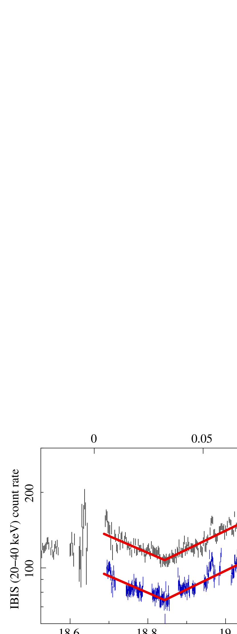
Figure 7: Light curves obtained with INTEGRAL-IBIS in the 20–40 keV band (top black data, left $y$ axis) and Suzaku-PIN in the 12–60 keV band (lower blue data, right $y$-axis) with a time resolution of 200 and 96 s, revealing an X-ray scattering trough shortly after superior conjunction, which lasts for 8.5 hours. During this time, the light curves can be described by two continuously jointed linear functions (red lines).

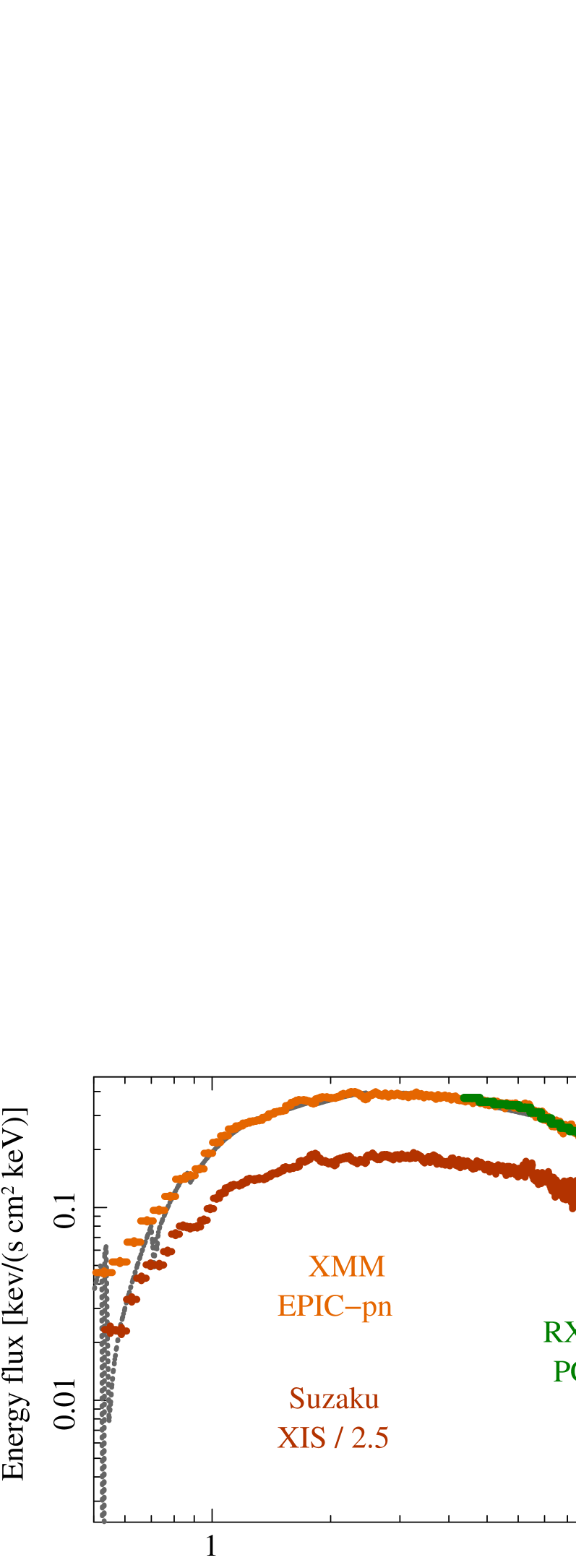
Figure 8: The 0.5 keV–2 MeV broadband spectrum of Cyg X-1, observed simultaneously with XMM, Suzaku, RXTE and INTEGRAL in 2008 April. The data below 300 keV can be described consistently by a broken power-law with exponential cutoff at high energies ($E_{\mathrm{fold}}\approx 170\,$keV). ISIS’ (model independent) flux-corrected spectra (relying on the response matrices) seem to indicate a non-thermal tail in the SPI data.

The broadband spectrum between 0.5 keV and 2 MeV, assembled from various instruments (Fig. 8), reveals that Cyg X-1 was again observed in the hard state. Below 300 keV, it can be described as a simple elbow-shaped broken power-law with high energy cutoff. RXTE-PCA’s photon indices below and above $E_{\mathrm{break}}=9.8\,$keV, namely $\Gamma_{1}=1.7$ and $\Gamma_{2}=1.4$, are amongst the hardest ones found in the long term monitoring of Cyg X-1 from 1999 to 2004 [16, 18]. Preliminary INTEGRAL-SPI data seem to indicate a non-thermal tail in the spectrum above 400 keV, but further analysis through joint broadband fits with Comptonization models is still ongoing.

- [1] M. Bałucińska-Church, M. J. Church, P. A. Charles, F. Nagase, J. LaSala, and R. Barnard, The distribution of X-ray dips with orbital phase in Cygnus X-1, MNRAS 311, 861–868 (2000).
- [2] J. M. Blondin, The shadow wind in high-mass X-ray binaries, ApJ 435, 756–766 (1994).
- [3] C. Brocksopp, A. E. Tarasov, V. M. Lyuty, and P. Roche, An improved orbital ephemeris for Cygnus X-1, A&A 343, 861–864 (1999).
- [4] J. I. Castor, D. C. Abbott, and R. I. Klein, Radiation-driven winds in Of stars, ApJ 195, 157–174 (1975).
- [5] D. B. Friend and J. I. Castor, Radiation-driven winds in X-ray binaries, ApJ 261, 293–300 (1982).
- [6] D. R. Gies and C. T. Bolton, The optical spectrum of HDE 226868 = Cygnus X-1. II. Spectrophotometry and mass estimates, ApJ 304, 371–388 (1986).
- [7] D. R. Gies and C. T. Bolton, The optical spectrum of HDE 226868 = Cygnus X-1. III. A focused stellar wind model for He II 4686 emission, ApJ 304, 389–394 (1986).
- [8] D. R. Gies, C. T. Bolton, J. R. Thomson, W. Huang, M. V. McSwain, R. L. Riddle, Z. Wang, P. J. Wiita, D. W. Wingert, B. Csák, and L. L. Kiss, Wind accretion and state transitions in Cygnus X-1, ApJ 583, 424–436 (2003).
- [9] M. Hanke, J. Wilms, M. A. Nowak, K. Pottschmidt, N. S. Schulz, and J. C. Lee, X-ray spectroscopy of the focused wind in the Cygnus X-1 system with Chandra. I. The non-dip spectrum in the low/hard state, ApJ (2008), in press (ArXiv:0808.3771).
- [10] M. Hanke, J. Wilms, M. A. Nowak, K. Pottschmidt, N. S. Schulz, and J. C. Lee, X-ray spectroscopy of the focused wind in the Cygnus x-1 system with Chandra II. The dip spectrum, ApJ (2009), in preparation.
- [11] A. Herrero, R. P. Kudritzki, R. Gabler, J. M. Vilchez, and A. Gabler, Fundamental parameters of galactic luminous OB stars. II. A spectroscopic analysis of HDE 226868 and the mass of Cygnus X-1, A&A 297, 556 (1995).
- [12] J. C. Houck and L. A. Denicola, ISIS: An interactive spectral interpretation system for high resolution X-ray spectroscopy in proceedings of Astronomical Data Analysis Software and Systems IX, (N. Manset, C. Veillet, and D. Crabtree, eds.), ASP Conf. Ser., no. 216, 2000, p. 591.
- [13] S. M. Kahn, M. A. Leutenegger, J. Cottam, G. Rauw, J.-M. Vreux, A. J. F. den Boggende, R. Mewe, and M. Güdel, High resolution X-ray spectroscopy of zeta Puppis with the XMM-newton Reflection Grating Spectrometer, A&A 365, L312–L317 (2001).
- [14] H. J. G. L. M. Lamers and C. Leitherer, What are the mass-loss rates of O stars?, ApJ 412, 771–791 (1993).
- [15] M. S. Noble and M. A. Nowak, Beyond XSPEC: Toward highly configurable astrophysical analysis, PASP 120, 821–837 (2008).
- [16] M. A. Nowak, Suzaku Observations of Cyg X-1 in proceedings of VII Microquasar Workshop: Microquasars and Beyond, 2008, (ArXiv:0810.1519).
- [17] D. Porquet and J. Dubau, X-ray photoionized plasma diagnostics with helium-like ions. Application to warm absorber-emitter in active galactic nuclei, A&AS 143, 495–514 (2000).
- [18] J. Wilms, M. A. Nowak, K. Pottschmidt, G. G. Pooley, and S. Fritz, Long term variability of Cyg X-1. IV. Spectral evolution 1999-2004, A&A 447, 245–261 (2006).