Transport Properties of Holographic Defects

Abstract:

We study the charge transport properties of fields confined to a (2+1)-dimensional defect coupled to (3+1)-dimensional super-Yang-Mills at large-$N_{\textrm{\tiny c}}$ and strong coupling, using AdS/CFT techniques applied to linear response theory. The dual system is described by $N_{\textrm{\tiny f}}$ probe D5- or D7-branes in the gravitational background of $N_{\textrm{\tiny c}}$ black D3-branes. Surprisingly, the transport properties of both defect CFT’s are essentially identical – even though the D7-brane construction breaks all supersymmetries. We find that the system possesses a conduction threshold given by the wave-number of the perturbation and that the charge transport arises from a quasiparticle spectrum which is consistent with an intuitive picture where the defect acquires a finite width. We also examine finite-$\lambda$ modifications arising from higher derivative interactions in the probe brane action.

1 Introduction

The AdS/CFT correspondence provides a powerful framework for the study of strongly coupled gauge theories [1, 2, 3]. While the gauge theories that are currently amenable to such holographic analysis are typically very different from real world QCD, this duality may still give us some insight into the strongly coupled quark-gluon plasma (sQGP) produced in recent experiments at RHIC [4]. Matching AdS/CFT results with experimental data here anticipates that the sQGP can be described by an effective CFT which is in the same universality class as the strongly coupled gauge theories studied holographically. Similar considerations have recently motivated exploring the possible application of the AdS/CFT correspondence to the study of $(2+1)$-dimensional condensed matter systems [5]. A variety of holographic models displaying interesting properties, including superfluidity, superconductivity and Hall conductivity, have now been studied [6, 7, 8]. Further interesting models of various types of nonrelativistic CFT’s have also been constructed [9]. One advantageous aspect of the AdS/CFT correspondence is the “uniformity” of the calculations, i.e., a single set of calculations describes the system in different disparate regimes ($\omega\rightarrow 0$ versus $T\rightarrow 0$). This can be contrasted with more conventional field theory analysis of conformal systems in (2+1)-dimensions [10]. One might also approach these explorations of possible “AdS/Condensed Matter” correspondences with some optimism because of the rich variety of experimental systems which might exhibit conformal behaviour and also the vast array of four-dimensional AdS vacua in the string theory landscape [11].

In the present paper, we use the AdS/CFT correspondence to study the charge transport properties of fields confined to a (2+1)-dimensional defect coupled to (3+1)-dimensional super-Yang-Mills. The defect CFT is realized by inserting $N_{\textrm{\tiny f}}$ probe D5- or D7-branes into the background of a black D3-brane. In either construction, we are also able to introduce an additional internal flux, in which case the defect in the CFT separates regions where the rank of the SYM gauge group is different. The defect CFT constructed with the D5-branes is certainly well known [12, 13, 14]. Certain aspects of the D7-brane construction have also been studied previously [15, 16] but we should note that the internal flux introduced here is essential to remove an instability that would otherwise appear in this construction. We will use linear response theory to study the conductivity on the defect at finite frequency and temperature and at finite wave-number, i.e., the conductivity of an anisotropic current.

An overview of the paper is as follows: In section 2, we review the holographic framework, in particular the embedding of the probe D-branes in the AdS${}_{5}\times S^{5}$ background. In section 3, we obtain the basic results for the spectral functions, starting with a review of the methodology and then the computation of the transverse and longitudinal conductivities in section 3.1. Here we also comment on the agreement with the diffusion-dominated conductivity in the hydrodynamic regime, i.e., in the regime at small frequency and wave-number $\omega,q\ll T$. This is followed by a discussion of the collisionless, ($q\mathrel{\raisebox{-2.58334pt}{$\stackrel{{\scriptstyle\textstyle>}}{{\sim}}$}}T$), regime using analytical approximations in section 3.2, for both the insulating case (at small fequencies) and the optical regime (at large frequencies). Using those results, we study the spectrum of quasinormal modes in section 4. In section 5, we examine the effect of stringy corrections to the gauge theory on the probe branes, which describes the behaviour of the dual currents on the defect. In particular, electromagnetic duality is lost when these $\alpha^{\prime}$-corrections are included, which has interesting implications for the conductivity as strong but finite ‘t Hooft coupling. Finally, we consider the computation of a topological Hall conductivity in section 6. Section 7 closes with some discussion and observations about our results. Some details of our analysis are relegated to appendices: In appendix A, we calculate the diffusion constant for charge transport. Appendix B presents some details of the analysis including certain $\alpha^{\prime}$ corrections in the D5-brane worldvolume action. In appendix C, we do an analytical study of a slightly simplified model of the defect, which gives further qualitative insight, and aids the numerical computation of the quasinormal modes.

2 Defect branes

The AdS/CFT correspondence is most studied and best understood as the duality between type IIb string theory on $AdS_{5}\times S^{5}$ and ${\cal N}=4$ super-Yang-Mills theory with $U(N_{\textrm{\tiny c}})$ gauge group. In this context, all fields in the SYM theory transform in the adjoint representation of the gauge group. One approach to introducing matter fields transforming in the fundamental representation is to insert probe D7-branes into the supergravity background [17]. However, this approach can also be used to construct a defect field theory, where the fundamental fields are only supported on a subspace within the four-dimensional spacetime of the gauge theory. In particular, we will consider constructing a $(2+1)$-dimensional defect by inserting $N_{\textrm{\tiny f}}$ D$p$-branes, with three dimensions parallel to the SYM directions and $p-3$ directions wrapped on the $S^{5}$. In the following, we work with both probe D5- and D7-branes. If we consider the supergravity background as the throat geometry of $N_{\textrm{\tiny c}}$ D3-branes, our defect constructions are described by the following array:

$$\begin{array}[]{rcccccccccccl}&&0&1&2&3&4&5&6&7&8&9&\\ \mathrm{background\,:}&D3&\times&\times&\times&\times&&&&&&&\\ \mathrm{probe\,:}&D5&\times&\times&\times&&\times&\times&\times&&&&\\ &D7&\times&\times&\times&&\times&\times&\times&\times&\times&&\\ \end{array}$$ (2.1)

The D5-brane construction is supersymmetric and the dual field theory is now the SYM gauge theory coupled to $N_{\textrm{\tiny f}}$ fundamental hypermultiplets, which are confined to a (2+1)-dimensional defect. Note that the supersymmetry has been reduced from ${\cal N}=4$ to ${\cal N}=2$ by the introduction of the defect. In the D7-brane case, we have lost supersymmetry altogether and the defect supports $N_{\textrm{\tiny f}}$ flavours of fermions, again in the fundamental representation [15]. One should worry that the lack of supersymmetry in the latter case will manifest itself with the appearance of instabilities. However, we will explicitly show below in section 2.2 that this problem can be avoided. In the limit $N_{\textrm{\tiny f}}\ll N_{\textrm{\tiny c}}$, the D5- and D7-branes may be treated as probes in the supergravity background, i.e., we may ignore the gravitational back-reaction of the branes.

As we commented above, a similar holographic framework has been used extensively to study the properties of the ${\cal N}=2$ gauge theory constructed with parallel D7- and D3-branes, i.e., the fundamental fields propagate in the full four-dimensional spacetime – e.g., see [18, 19, 20]. If a mass $M_{\textrm{\tiny q}}$ is introduced for the hypermultiplets, it was found that the scale $M_{\textrm{\tiny fun}}\sim M_{\textrm{\tiny q}}/\sqrt{\lambda}$ plays a special role in this theory. First, the “mesons”, bound states of a fundamental and an anti-fundamental field, are deeply bound with their spectrum of masses characterized by $M_{\textrm{\tiny fun}}$ [21]. Next at a temperature $T\sim M_{\textrm{\tiny fun}}$, the system undergoes a phase transition characterized by the dissociation of the mesonic bound states [20]. The analogous results can be verified for the defect theories considered here. That is, the meson spectrum is characterized by the same mass scale $M_{\textrm{\tiny fun}}$ [22, 23] and these states are completely dissociated in a phase transition at $T\sim M_{\textrm{\tiny fun}}$ [24]. However, these results are tangential to the present study, as we will only consider the conformal regime with $M_{\textrm{\tiny q}}=0$.

Common to both of our constructions is the supergravity background dual to ${\cal N}=4$ SYM at finite temperature. This background is a planar black hole in $AdS_{5}$, corresponding to the decoupling limit of $N_{\textrm{\tiny c}}$ black D3-branes [25]:

$$ds^{2}=\frac{r^{2}}{L^{2}}\left(-h(r)dt^{2}+dx^{2}+dy^{2}+dz^{2}\right)+\frac{L^{2}}{r^{2}}\left(\frac{dr^{2}}{h(r)}+r^{2}d\Omega_{5}^{2}\right)\,,\quad\quad C^{(4)}_{txyz}=-\frac{r^{4}}{L^{4}}$$ (2.2)

where $h(r)=1-r_{0}^{4}/r^{4}$. The gauge theory directions correspond the coordinates $\{t,x,y,z\}$. The radius of curvature $L$ is defined in terms of the string coupling constant $g_{\textrm{\tiny s}}$ and the string length scale $\ell_{\textrm{\tiny s}}$ as $L^{4}=4\pi\,g_{\textrm{\tiny s}}N_{\textrm{\tiny c}}\,\ell_{\textrm{\tiny s}}^{4}$. The holographic dictionary relates the Yang-Mills and string coupling constants as $g_{\textrm{\tiny YM}}^{2}=4\pi g_{\textrm{\tiny s}}$ and so we may write $L^{4}=\lambda\,\ell_{\textrm{\tiny s}}^{4}$ where $\lambda=g_{\textrm{\tiny YM}}^{2}N_{\textrm{\tiny c}}$ is the ’t Hooft coupling. As usual, we work in the supergravity approximation, ignoring the effects of string loops or higher derivative terms suppressed by powers of $\ell_{\textrm{\tiny s}}$ (except in section 5 and appendix B). Hence, we are working in the limit where both $N_{\textrm{\tiny c}},\,\lambda\rightarrow\infty$. The background (2.2) contains an event horizon at $r=r_{0}$. The temperature of the SYM theory is then equivalent to the Hawking temperature:

$$T=\frac{r_{0}}{\pi L^{2}}\,.$$ (2.3)

2.1 D5-branes

Introducing D5-branes as in (2.1) was the original application of probe branes for the holographic construction of a defect CFT – e.g., see [12, 13]. The worldvolume action which will determine the embedding of the probe D5-branes has the usual Dirac-Born-Infeld (DBI) and Wess-Zumino (WZ) terms:

$$I_{5}=-N_{\textrm{\tiny f}}\,T_{5}\int d^{6}\sigma\sqrt{-det\left(P[G]+2\pi\ell_{\textrm{\tiny s}}^{2}F\right)}+N_{\textrm{\tiny f}}\,T_{5}\int C^{(4)}\wedge 2\pi\ell_{\textrm{\tiny s}}^{2}F\,.$$ (2.4)

Implicitly we have assumed that the $N_{\textrm{\tiny f}}$ D5-branes are all coincident. Hence, in principle, their worldvolume supports a $U(N_{\textrm{\tiny f}})$ gauge theory, however, implicitly above and in the following, we only consider the gauge field in the diagonal $U(1)$ of this $U(N_{\textrm{\tiny f}})$. We choose coordinates on the five-sphere in (2.2) such that

$$d\Omega_{5}^{2}=d\psi^{2}+\cos^{2}\psi\left(d\theta^{2}+\sin^{2}\theta\,d\phi\right)+\sin^{2}\psi\,d{\Omega}_{2}^{2}\,.$$ (2.5)

The D5-branes wrap the two-sphere parameterized by $\{\theta,\phi\}$ above, fill three of the gauge theory directions $\{t,x,y\}$ and extend in the radial direction $r$. We also introduce a flux of the worldvolume gauge field on the two-sphere:

$$F_{\theta\phi}=\frac{q}{2\,N_{\textrm{\tiny f}}}\,\sin\theta\,.$$ (2.6)

One may verify that this flux corresponds to dissolving $q$ D3-branes into the worldvolume of the $N_{\textrm{\tiny f}}$ D5-branes along the $\{t,x,y,r\}$ directions, since the branes with flux sources $C^{(4)}$ through the WZ term in (2.4).

Now in general, the D5-brane embedding would be specified by giving its profile in both the angular direction $\psi(r)$ and the D3-brane direction $z(r)$. These embeddings all have translational symmetry in the $\{t,x,y\}$-space, as well as invariance under $SO(3)$ rotations on the internal two-sphere. In the following, we consider only the embeddings with $\psi=0$, i.e., where the D5-brane wraps a maximal two-sphere in the internal space. One can easily verify this choice corresponds to a solution of the worldvolume embedding equations. This choice also corresponds to setting the mass of the fundamental fields to zero, i.e., $M_{\textrm{\tiny q}}=0$, and so as we will describe below, this choice also ensures that the dual field theory with the defect remains conformal.

Hence in our analysis, we must determine the profile $z(r)$. The induced metric on the D5-branes is now described by

$$ds^{2}=\frac{r^{2}}{L^{2}}\left(-h(r)dt^{2}+dx^{2}+dy^{2}\right)+\left(\frac{L^{2}}{r^{2}h(r)}+\frac{r^{2}}{L^{2}}\partial_{r}z^{2}\right)dr^{2}+L^{2}\left(d\theta^{2}+\sin^{2}\theta\,d\phi\right)\,.$$ (2.7)

We can integrate over the two-sphere directions to produce a factor of

$$\oint_{S^{2}}d^{2}\sigma\sqrt{det_{S^{2}}\left(P[G]+2\pi\ell_{\textrm{\tiny s}}^{2}F\right)}=4\pi\,\left(N_{\textrm{\tiny f}}^{2}L^{4}+\pi^{2}\ell_{\textrm{\tiny s}}^{4}q^{2}\right)^{1/2}=4\pi N_{\textrm{\tiny f}}L^{2}\,\sqrt{1+f^{2}}$$ (2.8)

where

$$f\equiv\frac{\pi\ell_{\textrm{\tiny s}}^{2}}{L^{2}}\,\frac{q}{N_{\textrm{\tiny f}}}=\frac{\pi}{\sqrt{\lambda}}\frac{q}{N_{\textrm{\tiny f}}}$$ (2.9)

in the DBI part of the action (2.4). The full D5-brane action then becomes

$$I_{5}=-4\pi N_{\textrm{\tiny f}}\,T_{5}\sqrt{1+f^{2}}\int d^{3}x\,dr\,r^{2}\left(1+\frac{r^{4}}{L^{4}}h(r)\partial_{r}z^{2}\right)^{1\over 2}-4\pi N_{\textrm{\tiny f}}\,T_{5}\frac{f}{L^{2}}\int d^{3}x\,dr\,r^{4}\,\partial_{r}z\,.$$ (2.10)

To simplify the analysis, we introduce the following coordinates:

$$u=\frac{r_{0}}{r}\,,\qquad\qquad\chi=\frac{r_{0}}{L^{2}}z\,.$$ (2.11)

With this new notation, $h(u)=1-u^{4}$ and so the horizon is now at $u=1$ while the asymptotic region is reached when $u\rightarrow 0$. The worldvolume action can now be written as:

$$I_{5}=-4\pi r_{0}^{3}N_{\textrm{\tiny f}}\,T_{5}\int d^{3}x\,\frac{du}{u^{4}}\,\left[\sqrt{1+f^{2}}\left(1+h(u)\chi^{\prime 2}\right)^{1\over 2}+f\,\chi^{\prime}\right]\,,$$ (2.12)

where $\chi^{\prime}\equiv\partial_{u}\chi$. This expression is independent of $\chi$, such that the variation with respect to $\chi^{\prime}$ yields a constant of motion:

$$\frac{1}{u^{4}}\,\left[\sqrt{1+f^{2}}\frac{h(u)\chi^{\prime}}{\left(1+h(u)\chi^{\prime 2}\right)^{1/2}}+f\right]=C\,.$$ (2.13)

To avoid singular behaviour at the horizon, we need to fix the integration constant to be $C=f$. In this case, (2.13) yields

$$\chi^{\prime}=-\frac{f}{\sqrt{1+f^{2}u^{4}}}\,.$$ (2.14)

Given this expression, the profile $\chi(u)$ can be expressed in terms of an incomplete elliptic integral. However, in the following, it will sufficient to have a closed form expression for $\chi^{\prime}$. We illustrate some typical profiles in figure 1.

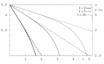
Figure 1: The brane profile $\chi$ for various values of $f$ at finite (solid) and zero (dashed) temperature. (Note the $T=0$ profiles correspond to $\chi=-f\,u$.)

In terms of our original coordinates, we have

$$\frac{\partial z}{\partial r}=\frac{L^{2}\,f}{\sqrt{r^{4}+f^{2}\,r_{0}^{4}}}\,.$$ (2.15)

Here we may consider the supersymmetric limit with $r_{0}=0$, in which case (2.15) simplifies to $z=-L^{2}f/r$. In this case, one can confirm that the induced metric (2.7) corresponds to AdS${}_{4}\times S^{2}$ with an AdS radius of curvature of $L_{{\rm AdS}_{4}}=L\,\sqrt{1+f^{2}}$ [12]. Hence the system inherits SO(2,3) symmetry from the AdS₄ geometry, which reflects the fact that the dual field theory remains conformal in the presence of the defect. This conformal invariance can also be shown directly by an analysis of the field theory [26]. Subsequently, the construction of the fully back-reacted geometries corresponding to the D5-branes embedded in $AdS_{5}\times S^{5}$ demonstrate that the preservation of the SO(2,3) symmetry is a fully nonperturbative result [14].

One may note that with the supersymmetric profile, $z=-L^{2}f/r$, there are an additional $q=\sqrt{\lambda}\,N_{\textrm{\tiny f}}\,f/\pi$ D3-branes stretching from $z=0$ to $-\infty$, assuming $f>0$. Hence if one were to include back-reaction, the asymptotic five-form flux would be shifted from $N_{\textrm{\tiny c}}\to N_{\textrm{\tiny c}}+q$ units on this side of the space. The same will apply at a finite temperature. Even though the brane falls through the horizon at a finite distance in this case, continuity at the horizon dictates that the background will carry $N_{\textrm{\tiny c}}+q$ units of flux out to $z=-\infty$. In either case, the natural interpretation is that the dual CFT has a $U(N_{\textrm{\tiny c}}+q)$ gauge group in the region $z<0$, while the gauge group remains $U(N_{\textrm{\tiny c}})$ for $z>0$.

It is interesting to pursue the interpretation of the above brane configuration in the dual CFT further. A detailed AdS/CFT dictionary has been developed for this defect system [13, 26]. In particular, one finds that the defect lagrangian contains potential source terms for the adjoint scalars in the SYM theory [13, 27]. The D5-brane carrying flux $f$ corresponds to producing a noncommutative configuration of adjoint scalars in a $U(q)$ subgroup of the $U(N_{\textrm{\tiny c}}+q)$ in the $z<0$ region [22]. In fact, in this supersymmetric configuration, the profile of the D5-branes can be precisely matched to the scalar profile using noncommutative geometry [28]: $r^{2}=(2\pi\ell_{\textrm{\tiny s}}^{2})^{2}\,{1\over N_{\textrm{\tiny f}}}{\rm Tr}(\Phi^{2})$ where ${1\over N_{\textrm{\tiny f}}}{\rm Tr}(\Phi^{2})={q^{2}\over 4N_{\textrm{\tiny f}}^{2}}\,{1\over z^{2}}$.

As the D5-brane wraps a maximal two-sphere inside the $S^{5}$, one might worry about the stability of this configuration. Indeed the worldvolume field, corresponding to fluctuations in the angle $\psi$, is found to be a tachyon with [12]

$$m^{2}_{\psi}=-\frac{2}{L^{2}(1+f^{2})}=-\frac{2}{L_{{\rm AdS}_{4}}^{2}}>-\frac{9}{4L_{{\rm AdS}_{4}}^{2}}\,.$$ (2.16)

However, the last inequality indicates that the $\psi$-mode satisfies the Breitenlohner-Freedman bound [29] in the asymptotically $AdS_{4}$ geometry induced on the D5-brane worldvolume. Hence this field does not in fact produce an instability.

Another concern may arise in considering the intersection of the D5-branes with the event horizon in (2.2). There we note that

$$\left.\chi^{\prime}\right|_{u=1}=-\frac{f}{\sqrt{1+f^{2}}}$$ (2.17)

or in terms of original coordinates

$$\left.\frac{\partial z}{\partial r}\right|_{r=r_{0}}=\frac{L^{2}\,f}{r_{0}^{2}\sqrt{1+f^{2}}}\,.$$ (2.18)

Since the D5-brane enters the event horizon at an angle, one might worry that the induced geometry is singular [30]. However, one can verify that this intuition is incorrect and that in fact, the D5-brane geometry remains smooth as it crosses the horizon. Hence the induced metric (2.7) describes a smooth ‘black hole’ geometry on the D5-brane worldvolume. A related question is: what is the surface gravity or the temperature of the induced horizon? It is a simple exercise to show that the relevant temperature matches that of the bulk geometry, i.e., that given in (2.3). Of course, this reflects the fact that the defect and bulk fields will be in thermal equilibrium, as expected.

We address one other potential concern related to the internal flux (2.6). Throughout the paper, we will be considering finite values of $f$, typically of $O(1)$. Hence according to (2.9), we are introducing $q\sim O(\sqrt{\lambda})$ D3-branes and so one might worry about whether it is reasonable to consider the probe brane limit, i.e., to ignore the gravitational back-reaction of the branes. Of course, this is not a problem since the overall tension of the D5-branes is not significantly modified by the flux, as can be seen from (2.10). The essential point is that the D3-branes are distributed on the D5-branes over the internal two-sphere which has an area of order $L^{2}\sim\sqrt{\lambda}$ and so the density of D3-branes remains small, i.e., the density is $O(f)$.

2.2 D7 probes

The case of D7 probe branes is similar to the previous section with D5-branes. The main difference lies in the internal part of the geometry. In particular, the D7-branes wrap a(n equatorial) four-sphere in the internal $S^{5}$. As before, we consider D3-branes dissolved into the probe branes. In the present case, the D7-branes source the three-brane charge through in the appropriate term in the WZ action: $\frac{1}{2}(2\pi\ell_{\textrm{\tiny s}}^{2})^{2}T_{7}\int C^{(4)}\wedge F\wedge F$. Hence, considering a stack of $N_{\textrm{\tiny f}}$ coincident D7-branes with a $U(N_{\textrm{\tiny f}})$ gauge symmetry, we introduce a nonvanishing second Chern class on the internal four-sphere: $q_{\textrm{\tiny 7}}=\frac{1}{8\pi^{2}}\oint_{S^{4}}TrF\wedge F$.

The D7-branes are fixed to wrap a maximal four-sphere while the embedding in the $AdS_{5}$ is described by $z=z(r)$. The induced metric on the D7-branes becomes

$$ds^{2}=\frac{r^{2}}{L^{2}}\left(-h(r)dt^{2}+dx^{2}+dy^{2}\right)+\left(\frac{L^{2}}{r^{2}h(r)}+\frac{r^{2}}{L^{2}}z^{\prime 2}\right)dr^{2}+L^{2}d\Omega_{4}^{2}\,.$$ (2.19)

Since the present configuration contains a nontrivial nonabelian gauge field, the worldvolume action requires a nonabelian extension of the DBI action [31]

$$I_{7}=-T_{7}\int d^{8}\sigma\,\mathrm{STr}\sqrt{-det\left(P[G]+2\pi\ell_{\textrm{\tiny s}}^{2}F\right)}+\frac{1}{2}T_{7}(2\pi\ell_{\textrm{\tiny s}}^{2})^{2}\int\mathrm{Tr}\left(C^{(4)}\wedge F\wedge F\right)\,.$$ (2.20)

This action uses the proposal of a maximally symmetric gauge trace, denoted by ‘STr’ [32]. To be precise, the trace includes a symmetric average over all orderings of $F_{ab}$ – and implicitly any appearances of the nonabelian scalars as well [33] but the latter will not be relevant in the present analysis. This prescription correctly agrees with the string action to fourth order in the field strength [32] but is known to miss certain commutator terms which begin to appear at sixth order [34]. However, the contribution of such terms is typically suppressed by factors of $1/N_{\textrm{\tiny f}}$ and so they can be safely neglected for sufficiently large $N_{\textrm{\tiny f}}$ [28, 35].

As before, we integrate over the internal space in the DBI action. Here the internal $S^{4}$ carries an nonabelian gauge field giving the instanton number $q_{\textrm{\tiny 7}}$. This configuration was extensively studied in [35] and hence using their results, we find

$$\oint_{S^{4}}d^{4}\Omega \mathrm{STr} \sqrt{det_{S^{4}}\left(P[G]+2\pi\ell_{\textrm{\tiny s}}^{2}F\right)}$$ (2.21)

$$= \oint_{S^{4}}d^{4}\Omega\,\sqrt{g_{S^{4}}}\,\sqrt{L^{8}+\frac{1}{2}L^{4}(2\pi\ell_{\textrm{\tiny s}}^{2})^{2}F_{ab}F^{ab}+\frac{1}{64}(2\pi\ell_{\textrm{\tiny s}}^{2})^{4}(\epsilon_{abcd}F^{ab}F^{cd})^{2}}$$

$$= \frac{8\pi^{2}}{3}\left(N_{\textrm{\tiny f}}\,L^{4}+6\pi^{2}\ell_{\textrm{\tiny s}}^{4}|q_{\textrm{\tiny 7}}|\right)\,.$$

In the latter, we use (anti-)self-duality for the instanton configuration: $F_{ab}=(-){1\over 2}\epsilon_{abcd}F^{cd}$ for $q_{\textrm{\tiny 7}}>0$ ($q_{\textrm{\tiny 7}}<0$). Implicitly, we are also assuming that the instanton number is uniform on the four-sphere, which limits $q_{\textrm{\tiny 7}}\leq N_{\textrm{\tiny f}}(N_{\textrm{\tiny f}}^{2}-1)/6$ [35]. Substituting (2.21) and the embedding (2.19) into (2.20), the action for the background configuration becomes

$$I_{7}=-\frac{8\pi^{2}N_{\textrm{\tiny f}}}{3}L^{4}(1+|Q|)T_{7}\int d^{3}\sigma dr\frac{r^{2}}{L^{2}}\sqrt{1+\frac{r^{4}}{L^{4}}h(r)}\,-\,\frac{8\pi^{2}N_{\textrm{\tiny f}}}{3}L^{4}Q\,T_{7}\int d^{3}\sigma dr\frac{r^{4}}{L^{4}}z^{\prime}\,,$$ (2.22)

where we defined for convenience $Q=6\pi^{2}\frac{\ell_{\textrm{\tiny s}}^{4}}{L^{4}}\frac{q_{\textrm{\tiny 7}}}{N_{\textrm{\tiny f}}}=\frac{6\pi^{2}}{\lambda}\frac{q_{\textrm{\tiny 7}}}{N_{\textrm{\tiny f}}}$. Now, the computations analogous to those in section 2.1 yield an identical embedding $\chi(u)$ as in (2.14) but the constant $f$ is replaced by

$$f_{7}\equiv\frac{Q}{\sqrt{1+2|Q|}}\,.$$ (2.23)

The microscopic interpretation of the D7-brane configuration in the dual CFT is not as clear in the present case. However, as before, the gauge group in the region $z<0$ will be enhanced to $U(N_{\textrm{\tiny c}}+q_{\textrm{\tiny 7}})$ assuming $q_{\textrm{\tiny 7}}>0$. There should be source terms on the defect which excite a noncommutative configuration of the adjoint scalars in the transverse space. The latter can be interpreted in terms of noncommutative geometry as giving the profile of the D7-branes, at least to leading order in $1/N_{\textrm{\tiny f}}$ [35].

An important difference between the present case and that in the previous section with D5-branes is that in the mass of the tachyonic mode $\psi$ corresponding to the $S^{4}$ part of the D7-branes “slipping off” the maximal $S^{4}$ in the internal space. A simple calculation reveals that

$$m^{2}_{\psi}\,=\,-\frac{4}{L^{2}(|Q|+1)}\,=\,-\frac{4}{L^{2}_{{\rm AdS}_{4}}}\,\frac{|Q|+1}{2|Q|+1}\,.$$ (2.24)

Recall that the BF bound requires $m^{2}>-\frac{9}{4L^{2}_{AdS_{4}}}$ [29] and hence is only satisfied for $|Q|>{\textstyle\frac{7}{2}}$. Hence one can trust the results in the following sections for the D7-branes only for $f_{7}^{2}>{49}/{32}$ and we might think of the internal flux on the $S^{4}$ as creating some pressure that stabilizes the size of the $S^{4}$. However, we should caution the reader that what we have shown is that the most obvious instability is removed for sufficiently large $Q$. While suggestive, this does not prove the D7-brane configuration is absolutely stable.

Beyond this crucial difference, the analysis of these two systems (i.e., defects constructed with D5- or D7-branes) is completely the same. Hence in the following, we focus on the first case of D5-branes and only comment on differences in coefficients that may arise for D7-branes where appropriate.

3 Correlators

In this section, we obtain examine various correlators of the currents dual to the worldvolume gauge field $A_{\mu}$. First we review the basic form of the correlators below, following [5]. Then we numerically compute the spectral functions in 3.1 and then examine the dependence of the correlators on the temperature and the flux $f$ in 3.2.

In the following, we use holographic techniques to calculate the retarded Green’s function for a conserved current $J_{\mu}(x)$ on the defect. The defect degrees of freedom form a (2+1)-dimensional CFT which restricts the form of the correlators:

$$C_{\mu\nu}(x-y)=-i\,\theta(x^{0}-y^{0})\,\langle\,[J_{\mu}(x),J_{\nu}(y)]\,\rangle\ ,$$ (3.25)

where translation invariance is assumed. The correlator can be Fourier transformed to $C_{\mu\nu}(p)$ with $p^{\mu}=(\omega,\vec{k})$. Now current conservation and rotational invariance (full Lorentz invariance is lost with $T>0$) restrict the form of the Fourier transform of this correlator to be [5]

$$C_{\mu\nu}(p)=P^{T}_{\mu\nu}\,\Pi^{T}(p)+P^{L}_{\mu\nu}\,\Pi^{L}(p)\,.$$ (3.26)

where the transverse and longitudinal projectors can be written as

$$P^{T}_{ij} = \delta_{ij}-\frac{k_{i}\,k_{j}}{k^{2}}\,,\qquad P^{T}_{0\mu}=0\,,$$

$$P^{L}_{\mu\nu} = \eta_{\mu\nu}-\frac{p_{\mu}\,p_{\nu}}{p^{2}}-P^{T}_{\mu\nu}\,.$$ (3.27)

If we take into account that the conformal dimension of the current $J_{\mu}(x)$ is 2, the components $\Pi^{T,L}$ in (3.26) take the form:

$$\Pi^{T,L}(p)=\sqrt{p^{2}}\,K^{T,L}(\omega/T,\vec{k}/T)\,.$$ (3.28)

In the limit of $T=0$, we have $\Pi^{T}(p)=\Pi^{L}(p)=\Pi(p)$ and recover the Lorentz invariant correlator

$$C_{\mu\nu}(p)=\left(\eta_{\mu\nu}-\frac{p_{\mu}\,p_{\nu}}{p^{2}}\right)\,\Pi(p)\,.$$ (3.29)

In order to produce physical observables, and to interpret our results from a condensed matter point of view, we will calculate the conductivity from the Kubo formula

$$\sigma_{ij}\,=\,\frac{i}{\omega}C_{ij}\ .$$ (3.30)

3.1 Spectral functions

In this section, we compute spectral functions for excitations of fundamental fields on the defect by studying fluctuations of the worldvolume fields on the D5-brane probes. In particular, we focus on correlators of the the worldvolume vector $A_{\mu}$, which is dual to the conserved current $J^{\mu}$ corresponding to the diagonal $U(1)$ of the global flavour symmetry on the defect. The worldvolume gauge field gives rise to several types of modes, one of which is a vector with respect to the Lorentz group in the (2+1)-dimensional defect. These modes are characterized as having only $A_{0,1,2}$ nonzero while the components on the internal two-sphere are vanishing [23]. Further the radial component $A_{r}$ can consistently be set to zero because we only study modes which are constant on the internal space [23].

While the full action for the gauge fields on the D5-branes receives contributions from both the Dirac-Born-Infeld (DBI) action plus a Wess-Zumino term, since our gauge field fluctuations have vanishing radial and $S^{2}$ components, only the DBI portion of the action is relevant in determining their dynamics. Since we only study linearized fluctuations about the background, the gauge field action is only needed to quadratic order, which is simply

$$I_{gauge}\,=\,-4\pi L^{2}\,\sqrt{1+f^{2}}N_{\textrm{\tiny f}}\,T_{5}\int d^{3}\sigma\,dr\sqrt{-g}\,\frac{(2\pi\ell_{\textrm{\tiny s}}^{2})^{2}}{4}\,F^{2}\,=\,-\frac{1}{4g_{4}^{2}}\int d^{3}\sigma\,dr\sqrt{-g}\,F^{2}\,.$$ (3.31)

Here we have integrated over the internal $S^{2}$ as in (2.8) and use $g_{\mu\nu}$ to denote the induced metric (2.7) in the AdS₅ directions. Above, we also defined the effective gauge coupling for the four-dimensional Maxwell field:

$$\frac{1}{g_{4}^{2}}\equiv 16\pi^{3}\ell_{\textrm{\tiny s}}^{4}L^{2}\,\sqrt{1+f^{2}}N_{\textrm{\tiny f}}\,T_{5}=\sqrt{1+f^{2}}\frac{2}{\pi}\,\frac{N_{\textrm{\tiny f}}\,N_{\textrm{\tiny c}}}{\sqrt{\lambda}}\,.$$ (3.32)

For the D7 case, this becomes

$$\frac{1}{g_{4}^{2}}\equiv\frac{32\pi^{4}N_{\textrm{\tiny f}}}{3}\ell_{\textrm{\tiny s}}^{4}L^{4}(1+|Q|)T_{7}=(1+|Q|)\frac{N_{\textrm{\tiny f}}\,N_{\textrm{\tiny c}}}{3\pi^{2}}\,.$$ (3.33)

Note that the gauge field action (3.31) corresponds to the standard Maxwell action in a four-dimensional curved spacetime. Hence, these gauge fluctuations will exhibit electromagnetic duality, which was shown to play and interesting role in the physics of the conformal field theory in [5]. We will explore this point further in section 5. Of course, Maxwell’s equations follow as

$$\partial_{a}\left({\sqrt{-g}}\,F^{ab}\right)=0.$$ (3.34)

Using these equations of motion, the Maxwell action (3.31) becomes a total derivative and following the standard prescription, we obtain the desired correlator from the resulting boundary term. To proceed, let us first give the explicit metric on the brane,

$$ds^{2}=\frac{L^{2}}{u^{2}}\left[\frac{r_{0}^{2}}{L^{4}}\big{(}-h(u)dt^{2}+dx^{2}+dy^{2}\big{)}+\frac{du^{2}}{h(u)}\left(1+h(u)\chi^{\prime 2}\right)\right]\,,$$ (3.35)

in terms of the dimensionless radial coordinate $u$, as given in (2.11). Then the action (3.31) becomes

$$I_{gauge} = -\frac{1}{2g_{4}^{2}}\int d^{3}\sigma\,du\,\partial_{a}\left[\sqrt{-{g}}\,A_{b}\,F^{ab}\right]\,=\,-\frac{1}{2g_{4}^{2}}\int d^{3}\sigma\,\left[\sqrt{-{g}}g^{aa}g^{uu}A_{a}\partial_{u}A_{a}\right]^{u\rightarrow 1}_{u\rightarrow 0}$$ (3.36)

$$= -\frac{1}{2g_{4}^{2}}\frac{r_{0}}{L^{2}}\int d^{3}\sigma\,\left[\frac{1}{(1+h(u)\chi^{\prime 2})^{1/2}}\left(h(u)A_{x}\partial_{u}A_{x}+h(u)A_{y}\partial_{u}A_{y}-A_{t}\partial_{u}A_{t}\right)\right]^{u\rightarrow 1}_{u\rightarrow 0}\ .$$

The usual AdS/CFT prescription tells us that we will only need the contribution at the asymptotic boundary $u\to 0$ [36]. Following [37], we take the Fourier transform of the gauge field,

$$A_{\mu}(\sigma)=\int\frac{d^{3}k}{(2\pi)^{3}}e^{ik\cdot\sigma}A_{\mu}(k,u)\,,$$ (3.37)

to write the boundary action as

$$I_{gauge} = -\frac{1}{2g_{4}^{2}1}\frac{1}{(2\pi)^{3}}\int d^{3}k\,\left[\sqrt{-{g}}g^{\mu\mu}g^{uu}A_{\mu}(u,-k)\partial_{u}A_{\mu}(u,k)\right]^{u\rightarrow 1}_{u\rightarrow 0}$$ (3.38)

$$= -\frac{r_{0}}{2g_{4}^{2}L^{2}}\frac{1}{(2\pi)^{3}}\int d^{3}k\,\left[(1+h(u)\chi^{\prime 2})^{-1/2}\left(h(u)A_{x}(u,-k)\partial_{u}A_{x}(u,k)\right.\right.$$

$$\qquad\qquad\left.\left.+h(u)A_{y}(u,-k)\partial_{u}A_{y}(u,k)-A_{t}(u,-k)\partial_{u}A_{t}(u,k)\right)\right]^{u\rightarrow 1}_{u\rightarrow 0}$$

with a single sum of $\mu$ being implicit in the first line.

Looking at the asymptotic behaviour of the fields, we write

$$A_{\mu}(k,u)=A_{\mu 0}(k)\frac{A_{\mu}(k,u)}{A_{\mu}(k,u_{0})}\,,$$ (3.39)

where $u_{0}$ is a UV regulator and it is understood that eventually the limit $u_{0}\to 0$ will be taken. We can then derive the flux factor for, say, $A_{y}$ by taking variations with respect to $A_{y0}$ [36]:

$$\mathcal{F}_{yy}=-\frac{\varepsilon_{0}}{2}\left[\frac{h(u)}{(1+h(u)\chi^{\prime 2})^{1/2}}\frac{A_{y}(u,-k)\partial_{u}A_{y}(u,k)}{A_{y}(u_{0},-k)A_{y}(u_{0},k)}\right]\,,$$ (3.40)

where $\varepsilon_{0}=\frac{r_{0}}{g_{4}^{2}L^{2}}=\frac{\pi\,T}{g_{4}^{2}}$ — we will show later how $\varepsilon_{0}$ relates to the charge permittivity. The flux (3.40) should be conserved, i.e., be independent of the radius $u$. The usual AdS/CFT prescription tells us to evaluate it at the asymptotic boundary, while applying infalling boundary conditions at the horizon ($u=1$), to find the retarded Green’s function (3.25) for the current $J_{\mu}$ in the defect CFT [36]:

$$C_{yy}=-2\mathcal{F}_{yy} = \varepsilon_{0}\left[\frac{h(u)}{(1+h(u)\chi^{\prime 2})^{1/2}}\frac{A_{y}(u,-k)\partial_{u}A_{y}(u,k)}{A_{y}(u_{0},-k)A_{y}(u_{0},k)}\right]_{u,u_{0}\to 0}$$ (3.41)

$$= \frac{\varepsilon_{0}}{\sqrt{1+f^{2}}}\left[\frac{\partial_{u}A_{y}(u,k)}{A_{y}(u,k)}\right]_{u\to 0}\,.$$

The other correlators $C_{\mu\nu}$ follow in general by rewriting (3.39) as $A_{\mu}(k,u)=A_{\nu 0}(k)M^{\nu}_{\ \mu}\!(u,k)$ [5] and making the variation $\frac{\delta^{2}}{\delta A_{\mu 0}\,\delta A_{\nu 0}}$. In our case the $t,t$ and $x,x$ correlators are given by (3.41) with the indices appropriately replaced:

$$C_{xx}\,=\,\frac{\varepsilon_{0}}{\sqrt{1+f^{2}}}\left[\frac{\partial_{u}A_{x}(u,k)}{A_{x}(u,k)}\right]_{u\to 0}\ \mathrm{and}\ \ C_{tt}\,=\,-\frac{\varepsilon_{0}}{\sqrt{1+f^{2}}}\left[\frac{\partial_{u}A_{t}(u,k)}{A_{t}(u,k)}\right]_{u\to 0}\,.$$ (3.42)

In order to evaluate the spectral function, we must solve the equations of motion (3.34). It is convenient to introduce dimensionless coordinates by rescaling the defect coordinates as

$${\tilde{t}}=\frac{r_{0}}{L^{2}}t\,,\qquad{\tilde{x}}=\frac{r_{0}}{L^{2}}x\,,\qquad{\tilde{y}}=\frac{r_{0}}{L^{2}}y\,.$$ (3.43)

Without loss of generality, we also assume the fluctuations only carry momentum in the ${\tilde{x}}$ direction, i.e., $\tilde{k}^{\mu}=(\tilde{\omega},\tilde{q},0)$ — note that, e.g., $\tilde{\omega}=L^{2}/r_{0}\ \omega=\omega/\pi\,T$. We note that given the Fourier transform (3.37), the vector potentials vary as $e^{i\tilde{k}_{\mu}{\tilde{x}}^{\mu}}$ in the gauge theory directions.

Now the explicit equations of motion simplify to

$$b=u:\qquad 0 = \tilde{\omega}A^{\prime}_{\tilde{t}}+\tilde{q}\,h\,A^{\prime}_{{\tilde{x}}}\,,$$ (3.44)

$$b={\tilde{t}}:\qquad 0 = A^{\prime\prime}_{\tilde{t}}-\frac{H^{\prime}}{2H}\,A^{\prime}_{\tilde{t}}-\frac{H}{h}\left(\tilde{q}^{2}A_{\tilde{t}}+\tilde{\omega}\tilde{q}A_{\tilde{x}}\right)\,,$$ (3.45)

$$b={\tilde{x}}:\qquad 0 = A^{\prime\prime}_{\tilde{x}}+\left(\frac{h^{\prime}}{h}-\frac{H^{\prime}}{2H}\right)\,A^{\prime}_{\tilde{x}}+\frac{H}{h^{2}}\left(\tilde{\omega}^{2}A_{\tilde{x}}+\tilde{\omega}\tilde{q}A_{\tilde{t}}\right)\,,$$ (3.46)

$$b={\tilde{y}}:\qquad 0 = A^{\prime\prime}_{\tilde{y}}+\left(\frac{h^{\prime}}{h}-\frac{H^{\prime}}{2H}\right)\,A^{\prime}_{\tilde{y}}+\frac{H}{h^{2}}(\tilde{\omega}^{2}-h\,\tilde{q}^{2})A_{\tilde{y}}\,,$$ (3.47)

where ‘prime’ denotes $\partial_{u}$ and

$$H(u)\equiv 1+h(u)\chi^{\prime 2}\,.$$ (3.48)

Before proceeding further, we make the following convenient definition for the conductivities

$$\tilde{\sigma}_{ij}\,\equiv\,\frac{i}{\tilde{\omega}}C_{ij}\,=\,\pi T\sigma_{ij}\ .$$ (3.49)

Comparing to (3.30), here we are simply dividing by the dimensionless frequency $\tilde{\omega}$, rather than $\omega$.

3.1.1 Transverse correlator

Let us look carefully at the ${\tilde{y}}$ equation (3.47). We see firstly, that in the limit $u\rightarrow 0$, it reduces to

$$0\,=\,A^{\prime\prime}_{\tilde{y}}+(1+f^{2})(\tilde{\omega}^{2}-\tilde{q}^{2})A_{\tilde{y}}\ .$$ (3.50)

The solution of interest is then $A_{\tilde{y}}=A_{{\tilde{y}}0}\,e^{-i\sqrt{(1+f^{2})(\tilde{\omega}^{2}-\tilde{q}^{2})}u}$, where the sign in the exponential is chosen so that the solution corresponds to an infalling wave. Given this solution, if one now calculates the correlator with (3.41) and applies (3.30), the resulting conductivity is

$$\tilde{\sigma}_{yy}=\varepsilon_{0}\sqrt{1-\tilde{q}^{2}/\tilde{\omega}^{2}}\,.$$ (3.51)

The cut in the conductivity at $\tilde{\omega}=\tilde{q}$ may be surprising and we return to this point in section 4.2. We will refer to this simple result as the low temperature approximation, reasoning as follows: The result applies for large dimensionless “frequencies”, i.e., $|(1+f^{2})(\tilde{\omega}^{2}-\tilde{q}^{2})|^{1/2}\gg 1$ to be precise. However, recalling that e.g., $\tilde{\omega}=\omega/\pi T$, if we fix the dimensionful quantities $\{\omega,q\}$, then eq. (3.51) should apply in the limit of very low temperatures.

To solve for the full spectral functions, we must proceed with numerical calculations. First, we impose infalling boundary conditions at the horizon — recall that the time-dependence of the potentials is $e^{-i\tilde{\omega}{\tilde{t}}}$. If we expand about $1-u\to 0^{+}$, we find an appropriate description of the field to be

$$A_{\tilde{y}}\simeq(1-u^{4})^{i\tilde{\omega}/4}\left(1+\beta(1-u)+\cdots\right)$$ (3.52)

where

$$\beta=\frac{i}{4}\tilde{\omega}\frac{3+5f^{2}}{1+f^{2}}+\frac{\tilde{q}^{2}}{\tilde{\omega}^{2}+4}\left(1-i\frac{\tilde{\omega}}{2}\right)\,.$$ (3.53)

In order to implement the infalling boundary condition and to ensure numerical stability, we choose the Ansatz

$$A_{\tilde{y}}=(1-u^{4})^{i\tilde{\omega}/4}e^{-\beta u}\mathcal{F}(u)\ ,$$ (3.54)

and solve for $\mathcal{F}(u)$, which is nonsingular at the horizon, with $\partial_{u}\mathcal{F}(u)=0$ at $u=1$. As the second boundary condition, we fix the asymptotic normalization: $A_{\tilde{y}}|_{u=1}=1$.

Figure 2: The normalized transverse conductivity ${\mbox{Re }}\tilde{\sigma}_{yy}(\tilde{\omega})/\varepsilon_{0}$ at $\tilde{q}\in\{1,2,3,4\}$ for various values of the flux $f$. The low temperature approximation (3.51) is shown as the dotted line for each $\tilde{q}$.

Figure 2 shows ${\mbox{Re }}\tilde{\sigma}_{yy}(\tilde{\omega})/\varepsilon_{0}$ for various values of $\tilde{q}$ and $f^{2}$. We see that at $f=0$ the spectral functions are similar to those in [5]. However, as $f$ increases, they approach the low temperature limit (3.51) more closely, and show some oscillatory behaviour at $\tilde{\omega}>\tilde{q}$. We will discuss aspects of this behaviour in section 3.2.

3.1.2 Longitudinal correlator

Now, let us consider the $tt$ equation (3.45). It is easy to see that (3.44-3.46) are not independent, and we cannot produce a second order equation involving $A_{\tilde{t}}$ only. However, we can produce one for $A^{\prime}_{\tilde{t}}$:

$$0\,=\,A^{\prime\prime\prime}_{\tilde{t}}\,-\,\Big{(}\frac{h}{H}\big{(}\frac{H}{h}\big{)}^{\prime}+\frac{H^{\prime}}{2H}\Big{)}A^{\prime\prime}_{\tilde{t}}\,+\,\Big{(}\frac{h}{H}\frac{H^{\prime}}{2H}\big{(}\frac{H}{h}\big{)}^{\prime}-\big{(}\frac{H^{\prime}}{2H}\big{)}^{\prime}\Big{)}A^{\prime}_{\tilde{t}}\,+\,\frac{H}{h^{2}}\big{(}\tilde{\omega}^{2}-\tilde{q}^{2}h\big{)}A^{\prime}_{\tilde{t}}\,,$$ (3.55)

which simplifies to

$$0=\left(\frac{A^{\prime}_{\tilde{t}}}{\sqrt{H}}\right)^{\prime\prime}+\left(\frac{h^{\prime}}{h}-\frac{H^{\prime}}{2H}\right)\,\left(\frac{A^{\prime}_{\tilde{t}}}{\sqrt{H}}\right)^{\prime}+\frac{H}{h^{2}}(\tilde{\omega}^{2}-h\,\tilde{q}^{2})\frac{A^{\prime}_{\tilde{t}}}{\sqrt{H}}\ ,$$ (3.56)

and hence is the same as (3.47) for $A_{\tilde{y}}$ replaced by $A^{\prime}_{\tilde{t}}/\sqrt{H}$. Let us set $A^{\prime}_{\tilde{t}}=c\,\sqrt{H}\,A_{\tilde{y}}$ with some constant $c$ to be determined. Now, to find ${\partial_{u}A_{\tilde{t}}(u,k)}/{A_{\tilde{t}}(u,k)}$ at $u=0$, we employ (3.45) and $A^{\prime\prime}_{\tilde{t}}=c\sqrt{H}\big{(}A^{\prime}_{\tilde{y}}+\frac{H^{\prime}}{2H}A_{\tilde{y}}\big{)}$ as in [5]. It follows then from $h^{\prime}|_{u=0}=0=H^{\prime}|_{u=0}$ that

$$c=\frac{\sqrt{1+f^{2}}}{A^{\prime}_{\tilde{y}}|_{u=0}}\left(\tilde{q}^{2}A_{{\tilde{t}}0}+\tilde{\omega}\tilde{q}A_{{\tilde{x}}0}\right)\,.$$ (3.57)

Hence, we can read off $\left[\frac{\partial_{u}A_{\tilde{t}}(u,k)}{A_{\tilde{t}}(u,k)}\right]_{u\to 0}$ and $\left[\frac{\partial_{u}A_{\tilde{t}}(u,k)}{A_{\tilde{x}}(u,k)}\right]_{u\to 0}$ from

$$A^{\prime}_{\tilde{t}}=\frac{\sqrt{1+f^{2}}\sqrt{H}A_{\tilde{y}}}{A^{\prime}_{\tilde{y}}|_{u=0}}\left(\tilde{q}^{2}A_{{\tilde{t}}0}+\tilde{\omega}\tilde{q}A_{{\tilde{x}}0}\right)\ .$$ (3.58)

Finally as in [5], we find

$$C_{tt}=-\varepsilon_{0}^{2}\,\tilde{q}^{2}/C_{yy}\qquad\mathrm{and}\qquad C_{xx}=-\varepsilon_{0}^{2}\,\tilde{\omega}^{2}/C_{yy}\,.$$ (3.59)

Applying (3.49), these results yield interesting relations for the corresponding conductivities. In particular, (3.59) yields

$$\tilde{\sigma}_{xx}=\varepsilon_{0}^{2}/\tilde{\sigma}_{yy}\ .$$ (3.60)

We can also consider a low temperature limit as above. However, this is most easily derived by combining (3.51) and (3.60) to find

$$\tilde{\sigma}_{xx}=\frac{\varepsilon_{0}}{\sqrt{1-\tilde{q}^{2}/\tilde{\omega}^{2}}}\,.$$ (3.61)

Again, we will return to discuss the cut appearing in the conductivity at $\tilde{\omega}=\tilde{q}$ in section 4.2; and the conductivity can only be found in general from numerical calculations. Some typical results for (the real part of) $\tilde{\sigma}_{xx}$ are shown in figure 3. We note that again that as the flux $f$ increases, our results approach the low temperature approximation (3.61), together with some “oscillatory” behaviour similar to that found in the transverse case. In contrast to the results in the previous section, the conductivity here diverges as $\tilde{\omega}\to\tilde{q}$, as can be anticipated from (3.61).

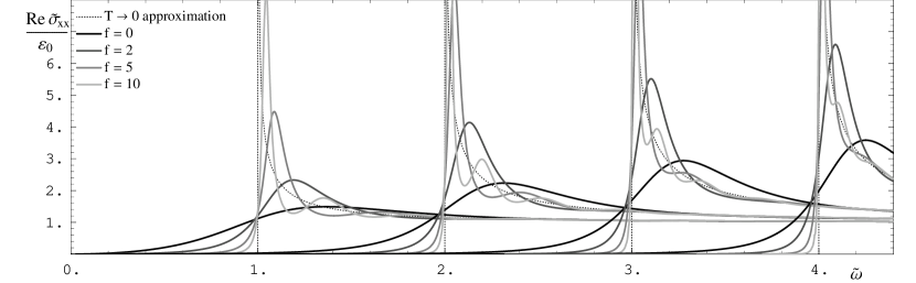
Figure 3: The normalized longitudinal conductivity ${\mbox{Re }}\tilde{\sigma}_{xx}(\tilde{\omega})/\varepsilon_{0}$ at $\tilde{q}\in\{1,2,3,4\}$ for various values of the flux $f$. The low temperature approximation (3.61) is shown as the dotted line for each $\tilde{q}$.

We can find the permittivity $\varepsilon$ from the hydrodynamic limit $T\gg\omega,q$ [38],

$$-\,{\mbox{Im }}C_{tt}\,=\,\frac{\varepsilon D\,\omega q^{2}}{\omega^{2}+(Dq^{2})^{2}}\,=\,\frac{\varepsilon\,\pi DT\,\tilde{\omega}\tilde{q}^{2}}{\tilde{\omega}^{2}+(\pi\,DT\,\tilde{q}^{2})^{2}}\,.$$ (3.62)

In this regime, the spectral function is dominated by the diffusion pole $\tilde{\omega}=-i\pi\,DT\,\tilde{q}^{2}$, as dictated by Fick’s law (A.100). The diffusion constant is $D=\frac{\sqrt{1+f^{2}}}{\pi T}I(f)$, as we calculate in appendix A, where we also define the function $I(f)$. Comparing to our numerical results for the spectral functions as shown in figure 4 for various values of $f$ and $\tilde{q}\ll 1$, we find $\varepsilon=\frac{\varepsilon_{0}}{I(f)}$. We can verify the latter from the definition of the permittivity [39],

$$\varepsilon\,=\,\frac{1}{T}\lim_{\tilde{\omega},\tilde{q}\to 0}C_{tt}\,,$$ (3.63)

which is in perfect agreement with the numerical result.

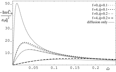
Figure 4: $\frac{-{\mbox{Im }}\tilde{C}_{tt}(\tilde{\omega})}{\varepsilon_{0}\tilde{q}^{2}}$ for $f\in\{0,4\}$ and $\tilde{q}\in\{0.1,0.2\}$. The solid lines correspond the approximate result (3.62) with only the diffusion pole appearing in the hydrodynamic limit.

3.2 Temperature and $f$ dependence

In the previous sections, we found an interesting dependence of the conductivity on the temperature and the flux $f$. These properties characterize the nature of the defect, as shown more in detail in figure 5. There we see that at low $T$ or large $f$, there is a conduction threshold at $\omega=q$. We can interpret this as the energy required to excite a collective excitation of the conducting mode. In the regime $\omega<q$, the conductivity appears exponentially suppressed as one might expect with a chemical potential $q$. That is, this exponential suppression in the low-temperature “DC limit” might be interpreted as the Boltzmann tail of some thermal distribution function. Examining this behaviour in more detail in the next section suggests the introduction of an effective temperature, which seems to play an interesting role in the subsequent analysis. Examining the conductivity at low $T$ or large $f$ also reveals “oscillations” in the spectral curves. The frequency of this oscillations has a non-trivial dependence on $f$ and seems to depend inversely on the temperature, as one might expect from the general scaling properties. Their amplitude is roughly independent of $f$, but depends on some positive power of the temperature and decreases with increasing $\frac{\tilde{\omega}}{\tilde{q}}$. In the following, we will also extract some quantitative approximation to this pattern.

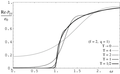
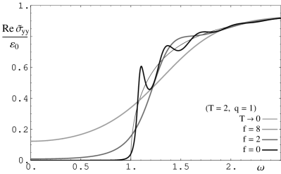
Figure 5: On the left, we plot the normalized transverse conductivity ${\mbox{Re }}\tilde{\sigma}_{yy}(\omega)/\varepsilon_{0}$ for $q=1$ and $f=2$ at various temperatures, in terms of the frequency $\omega$. On the right: ${\mbox{Re }}\tilde{\sigma}_{yy}(\omega)/\varepsilon_{0}$ for $q=1$ and $T=2$ for various values of $f$. In both plots, the $T\rightarrow 0$ limit (3.51) is shown with the narrow black curve.

First, we study these two effects analytically as a perturbation around the zero temperature limit. Next, we will show how they arise from poles in the spectral functions that can be interpreted in the field theory as the quasiparticle states of the resonances on the defect and arise on the gravity side through the quasinormal modes of the vector field. Finally, we will demonstrate the latter by reconstructing the location of the poles in the complex frequency plane from the data on the real axis and also by analytically solving a toy model that is very similar to our present problem.

3.2.1 Effective temperature

First let us study the temperature dependence of the DC limit. This can be easily done by finding an approximate solution in the $q\gg T$ limit. For simplicity, we will also take $\omega\ll T$. We will concentrate on the transverse correlators, but we will see that the conductivity is obtained from a small perturbation around a large background, such that by (3.59), a similar behaviour applies to the longitudinal correlator in the limit that we will consider. Before proceeding, it is useful to recall here that $h(u)\equiv 1-u^{4}$ while $H(u)$ is given by (3.48), so that asymptotically as $u\rightarrow 0$, $H\rightarrow\sqrt{1+f^{2}}$ while near the horizon where $u\rightarrow 1$, $H\rightarrow 1$.

Let us first re-express (3.47) in terms of the Ansatz $A_{\tilde{y}}=A_{{\tilde{y}}0}\,e^{\int^{u}\zeta}$, such that $C_{yy}=\frac{\varepsilon_{0}}{\sqrt{1+f^{2}}}\lim_{u\rightarrow 0}\zeta$:

$$\zeta^{\prime}+\zeta^{2}\,+\,\left(\frac{h^{\prime}}{h}-\frac{H^{\prime}}{2H}\right)\zeta+\frac{H}{h}\left(\frac{\tilde{\omega}^{2}}{h}-\tilde{q}^{2}\right)\,=\,0\ .$$ (3.64)

We see that for large $\tilde{q}$ (i.e., $q\gg T$), this equation is dominated by the second and last terms, such that an approximate solution is $\zeta=\pm\zeta_{0}$, $\zeta_{0}\equiv\tilde{q}\sqrt{\frac{H}{h}}$. Implicitly, here we have chosen the branch corresponding to $A_{\tilde{y}}$ decaying near the horizon. Further, as we will see below, this also corresponds to an infalling boundary condition at the horizon. The terms that we ignored are then of the order $\tilde{q}h^{-3/2}$, such that the approximation is valid in the region $1-u\gg\tilde{q}^{-2}$. The subleading terms in $\zeta$ are of the order $\tilde{q}^{0}u^{3}h^{-1}$.

Next, we study the linearized equation for a small perturbation $\zeta\rightarrow\zeta_{0}+\epsilon$:

$$\epsilon^{\prime}\,+\,\epsilon\left(\frac{h^{\prime}}{h}-\frac{H^{\prime}}{2H}-2\zeta_{0}\right)\,+\,\frac{\tilde{\omega}^{2}H}{h^{2}}-\zeta_{0}^{\prime}+\left(\frac{h^{\prime}}{h}-\frac{H^{\prime}}{2H}\right)\zeta_{0}\,\equiv\,\epsilon^{\prime}\,-\,\epsilon\alpha(u)\,-\,\beta(u)$$ (3.65)

with the general solution

$$\epsilon\,=\,e^{\int_{0}^{u}\!d\bar{u}\,\alpha(\bar{u})}\left(\epsilon_{0}\,+\,\int_{0}^{u}\!d\acute{u}\,e^{-\int_{0}^{\acute{u}}\!d\bar{u}\,\alpha(\bar{u})}\beta(\acute{u})\right)\ .$$ (3.66)

In the limit that we considered for $\zeta_{0}$ this reduces simply to $\epsilon\,=\,\epsilon_{0}e^{2\int_{0}^{u}\!d\bar{u}\,\zeta_{0}}$ because of the exponential suppression in the last term in (3.66). As one would have physically expected, this perturbation grows as one approaches the horizon, and decays away near infinity. The subleading terms from the part of $\alpha(u)$ that we ignored in the integral in the exponent is again of order $\tilde{q}^{0}u^{3}h^{-1}$.

To find $\epsilon_{0}$, fix the $\omega$ dependence and further constrain the subleading terms, we proceed by considering an approximate solution in the region $h=1-u^{4}\ll 1$, which has overlap with $h\gg\tilde{q}^{-2}$. The equation we need to solve is now

$$4\partial_{h}\zeta\,-\,\zeta^{2}\,+\,\frac{4}{h}\zeta\,+\,\frac{\tilde{q}^{2}}{h}-\frac{\tilde{\omega}^{2}}{h^{2}}\,=\,0\,,$$ (3.67)

which has a general analytic but not very illuminating solution in terms of Bessel functions, allowing for a combination of infalling and outgoing waves at the horizon $u=1$. Choosing an infalling boundary condition leaves us with

$$\zeta\,=\,-\frac{\tilde{q}^{2}h\,{}_{0}\!F_{1}\big{(}2+i\frac{\tilde{\omega}}{2};\tilde{q}^{2}\frac{h}{16}\big{)}\,-\,16i\frac{\tilde{\omega}}{2}\big{(}2+i\frac{\tilde{\omega}}{2}\big{)}{}_{0}\!F_{1}(2+i\frac{\tilde{\omega}}{2};\tilde{q}^{2}\frac{h}{16})}{8h\big{(}2+i\frac{\tilde{\omega}}{2}\big{)}{}_{0}\!F_{1}\big{(}1+i\frac{\tilde{\omega}}{2};\tilde{q}^{2}\frac{h}{16}\big{)}}\ ,$$ (3.68)

where ${}_{0}\!F_{1}(a;x)$ is the confluent hypergeometric limit function [40]. To match with the $h\ll 1$ regime of the asymptotic solution, we begin by expanding to first order in $\tilde{\omega}$ and then do an expansion around $\tilde{q}^{2}h\gg 1$, which gives us

$$\zeta\,\sim\,-\frac{\tilde{q}}{\sqrt{h}}+\frac{1}{h}+\cdots\,-\,i\tilde{\omega}\tilde{q}\frac{16\pi}{\sqrt{h}}e^{-\tilde{q}\sqrt{h}}\,+\,\cdots\ .$$ (3.69)

Hence the full solution for $h\gg\tilde{q}^{-2}$ is:

$$\zeta\,=\,-\tilde{q}\sqrt{\frac{H}{h}}+\frac{1}{h}+A(u,\tilde{q},f)\,-\,i\tilde{\omega}\tilde{q}\frac{16\pi}{\sqrt{h}}e^{-2\tilde{q}\int_{u}^{1}\sqrt{\frac{H}{h}}}\big{(}1+B(u,\tilde{q},f)\big{)}\ ,$$ (3.70)

where $A(u,\tilde{q},f)$ is some function that behaves away from the horizon as $\leq\mathcal{O}(u^{3},\tilde{q}^{0})$ and $B(u,\tilde{q},f)$ behaves as $\leq\mathcal{O}(u^{0},\tilde{q}^{0})$. Near the horizon, i.e., for $h\ll\tilde{q}^{-2}$, the solution behaves as $\zeta\sim-i\frac{\tilde{\omega}}{h}-\frac{2-i\tilde{\omega}}{8+2\tilde{\omega}^{2}}+\cdots$. As a consistency check in the region $1\gg h\gg\tilde{q}^{-2}$, it is easy to verify that the (small) imaginary and (dominating) real parts do indeed satisfy (3.66) when taking into account the next-to-leading terms.

From (3.70), we find that the leading term in the conductivity is

$$\sigma_{yy}\sim 16\pi\varepsilon_{0}\tilde{q}\,e^{-2\tilde{q}\int_{u}^{1}\sqrt{\frac{H}{h}}}\ .$$ (3.71)

Inspired by a Boltzmann factor, and by the zero-temperature conduction threshold $\omega_{0}=q$, we can interprete the exponential factor as $\exp[-{q}/{T_{eff}}]$ where

$$T_{eff}\,=\,\frac{\pi}{2}\,T\,\left(\int_{0}^{1}du\sqrt{\frac{H(u)}{h(u)}}\right)^{-1}\ .$$ (3.72)

We note that the integral is finite since the integrand converges as $h^{1/2}$ at $u\to 1$. There are two limits in which we can evaluate this integral analytically: $f=0$ and $f\gg 1$. In these limits one finds

$$f=0: T_{eff}=T\frac{\sqrt{\pi}}{2}\,\frac{\Gamma\left(\frac{3}{4}\right)}{\Gamma\left(\frac{5}{4}\right)}\sim 1.198\,T$$ (3.73)

$$f\gg 1: T_{eff}\simeq\frac{\Gamma\left({3}/{4}\right)^{2}}{\sqrt{\pi}}\frac{T}{\sqrt{f}}\left(1+\left(\frac{4\Gamma(3/4)^{2}}{\pi^{3/2}}-\frac{1}{\sqrt{2}}\right)\frac{1}{\sqrt{f}}\right)$$

$$\qquad\ \sim 0.847\,\frac{T}{\sqrt{f}}\left(1+0.372/\sqrt{f}\right)\ .$$

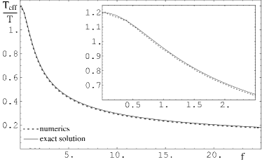
Figure 6: Ratio of the “effective temperature” derived from the temperature and $\tilde{q}$ dependence at $\tilde{q}\gg 1\gg\tilde{\omega}$ to the blackhole temperature as a function of the flux $f$. We show the exact expression derived from the $\tilde{q}\rightarrow\infty$ limit and the numerical estimate at finite $\tilde{q}$.

Comparing these results with the numerics, we find good convergence in a consistent manner of both the profile of $A_{y}(u)$ and the effective temperature with increasing $\tilde{q}$. Since the approximation that gave us the integrand in (3.72) is valid up to roughly $h\gtrsim\tilde{q}^{-2}$, we expect that $T_{eff}/T$ measured at finite $\tilde{q}$ has a relative accuracy of roughly $\tilde{q}^{-1}$. A simple way to estimate the effective temperature from the conductivity is to compute $\partial_{\tilde{q}}\log\frac{\tilde{\sigma}_{yy}}{\tilde{q}}\sim\frac{\pi}{T_{eff}}$ at large values of $\tilde{q}$. The factor of $\tilde{q}^{-1}$ that we have included here ensures that the convergence to the actual value of $T_{eff}$ is faster than logarithmic in $\tilde{q}$. In figure 6, we show the comparison to the numerical estimate computed at $q/T_{eff}\sim 47$, that is the best numerically stable estimate, and demonstrate how the estimates converge to the exact results.

As illustrated in figure 6, our new effective temperature does not match the actual temperature of the system, except for $f\simeq 0.85$. At this point, we emphasize that, as discussed in section 2, the degrees of freedom on the defect are in equilibrium with the thermal bath of adjoint fields with temperature $T$. Of course, $T_{eff}$ is still a scale that seems to play an interesting role in the defect conformal field theory, as we will see in the following. Again, the reason that we assign this scale the appellation of “effective temperature” is that it appears to play the role of a temperature when the conductivity (3.71) is interpreted as a Boltzmann distribution. It would be interesting if one could also give a physical interpretation to the pre-factor $16\pi\tilde{q}$ in front of the exponential in (3.71).

3.2.2 Resonances on the defect

Next, we study the oscillatory behaviour of the spectral functions at $\tilde{\omega}>\tilde{q}$, using two different methods. Our results for the transverse correlator $C_{yy}$ obviously can also be translated to give us the longitudinal correlators $C_{xx},C_{tt}$ using (3.59). Hence we will only discuss the former case.

We begin with the WKB-like expansion that gave (3.65), which was the starting point for the effective temperature above. Now however, we do not have the scale $h\sim\tilde{q}^{2}$ where we can match the near-horizon approximation to the asymptotic approximation. Furthermore, the dominant solution for $\epsilon$ is now oscillatory since $\zeta\sim\zeta_{0}=i\frac{\sqrt{H}}{h}\omega\sqrt{1-h\frac{\tilde{q}^{2}}{\tilde{\omega}^{2}}}$, rather than exhibiting the exponential decay found above. The latter also reduces the validity of the approximation that led to (3.65) and further we have to worry about the logarithmically diverging integral $\int\zeta_{0}\propto\ln h$ as $u\to 1$. So let us take the solution (3.66), but now with

$$\zeta_{0}=i\frac{\sqrt{H}}{h}\omega\sqrt{1-h\frac{\tilde{q}^{2}}{\tilde{\omega}^{2}}}\,,\ \ \alpha=2\zeta_{0}-\left(\ln\frac{h}{\sqrt{H}}\right)^{\prime}\,,\ \ \beta=\zeta_{0}^{\prime}+\left(\ln\frac{h}{\sqrt{H}}\right)^{\prime}\zeta_{0}\,$$ (3.75)

and match this in the limit $u\rightarrow 1$ to the appropriate expansion of (3.68):

$$\zeta\,\sim\,-\frac{i\tilde{\omega}}{h}\,+\,\frac{i\tilde{q}^{2}}{2\tilde{\omega}-4i}\,+\mathscr{O}(h)\,=\,-\zeta_{0}\,+\,\frac{\tilde{q}^{2}}{\tilde{\omega}^{2}+2i\tilde{\omega}}\,+\,\mathscr{O}(h)\,.$$ (3.76)

Now, we see that the divergent oscillations from the $e^{\int\alpha}$ terms in (3.66) must cancel, and the approximation $\epsilon\ll\zeta_{0}$ should be valid near the horizon. Taking the limit $\lim_{u\to 1}\epsilon=\frac{\tilde{q}^{2}}{\tilde{\omega}^{2}+2i\tilde{\omega}}\equiv\epsilon_{H}$ of (3.66), and solving for $\epsilon_{0}$ gives us then

$$\epsilon|_{u=0}\,=\,\epsilon_{0} = \epsilon_{H}e^{-\int_{0}^{1}du\alpha(u)}\,+\,\int_{0}^{1}du\epsilon_{H}e^{-\int_{0}^{u}d\tilde{u}\alpha(\tilde{u})}\beta(u)$$ (3.77)

$$= \epsilon_{H}\,-\,\int_{0}^{1}du\,h\sqrt{\frac{1+f^{2}}{H}}e^{-2\int_{0}^{u}d\tilde{u}\zeta_{0}}\left(\epsilon_{H}\alpha-\frac{1}{2}\zeta_{0}\frac{h^{\prime}\tilde{q}^{2}/\tilde{\omega}^{2}}{1-h\tilde{q}^{2}/\tilde{\omega}^{2}}\right)\,.$$

It turns out that the $\mathscr{O}(h^{-1})$ divergent terms in $\epsilon_{H}\alpha+\beta$ in (3.77) do indeed cancel, such that the integral converges with the integrand $\propto h^{2}h^{i\tilde{\omega}/2}$ as $u\to 1$. Unfortunately, we were not able to evaluate this integral analytically, even in the limits where various quantities involved getting large or small. We show this approximate result (3.77) compared to the full numerical result in figure 8.

Because of the rapid convergence as $u\to 1$, we see however that most of the contribution to the integral comes from regions where $h\sim 1$, in particular for large $f$. Hence as a very crude approximation, we can set $h=1$ and hence $\beta=0$, which allows us to compute the integral analytically:

$$\epsilon_{0}\,\sim\,\epsilon_{H}\sqrt{1+f^{2}}e^{-2i\tilde{\omega}\sqrt{1+f^{2}}I(f)\sqrt{1-\tilde{q}^{2}/\tilde{\omega}^{2}}}\ .$$ (3.78)

While we do not expect this latter expression to give us the correct phase and amplitude information, we still anticipate that this result gives a good approximation for the frequency of the oscillations, $2\sqrt{1+f^{2}}I(f)\sqrt{1-\tilde{q}^{2}/\tilde{\omega}^{2}}$.

There is an alternative way of seeing more physically from the bulk point of view, how the finite temperature effects arise by casting the equation of motion for $A_{y}$ (3.47) in the form of the Schrödinger equation, as suggested in [41]:

$$\left(-\partial_{\rho}^{\,2}+h\,\tilde{q}^{2}\right)A_{y}\,=\,\tilde{\omega}^{2}A_{y}\qquad{\rm where}\ \ \rho\,=\,\int_{0}^{u}d\tilde{u}\frac{\sqrt{H}}{h}\ .$$ (3.79)

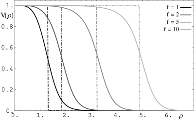
Figure 7: The effective Schrödinger potential $V(\rho)=\tilde{q}^{2}h$ for the gauge field on the brane. We set $\tilde{q}=1$ in the plot.

In terms of this new radial coordinate, the horizon gets mapped to $\rho\to\infty$, and we see that $\rho$ is rapidly varying only for $u\lesssim f^{-1/2}$ and for $h\ll 1$. This suggests that for large $f$ we can approximately split the problem in two regions: An asymptotic one where $h\sim 1$ and $\rho\sim\rho_{\infty}(u)=\int_{0}^{u}d\tilde{u}\sqrt{H}$ and the near-horizon region, where $h\ll 1$ and $\rho\sim\rho_{H}(u)=\rho_{0}-\frac{1}{4}\ln(h)$ for some $\rho_{0}$. Going even further in our approximation, we assume a square potential $V=\tilde{q}^{2}$ for $\rho<\rho_{\infty}(1)=\sqrt{1+f^{2}}I(f)$ and $V=0$ for $\rho>\rho_{\infty}(1)$, which is displayed in figure 7, where we see that this approximation is indeed justified. At this point, we might also observe that the effective Schrödinger potential appearing here is very similar in structure to that found for supergravity modes [42] and for mesonic modes, as discussed in [43].

With the square potential, it is trivial to find the solution for infalling boundary conditions at the horizon:

$$A_{y}\,\sim\,\left\{\begin{array}[]{lll}{\textstyle A_{0}\,2\sqrt{1-\tilde{q}^{2}/\tilde{\omega}^{2}}e^{-i\tilde{\omega}(\rho-\sqrt{1+f^{2}}I(f))}}&:&\rho<\sqrt{1+f^{2}}I(f)\\ {\textstyle A_{0}\Big{(}\big{(}1+\sqrt{1-\tilde{q}^{2}/\tilde{\omega}^{2}}\big{)}e^{-i\tilde{\omega}\sqrt{1-\tilde{q}^{2}/\tilde{\omega}^{2}}(\rho-\sqrt{1+f^{2}}I(f))}}&&\\ \ \ \ \ \ {\textstyle-\big{(}1-\sqrt{1-\tilde{q}^{2}/\tilde{\omega}^{2}}\big{)}e^{i\tilde{\omega}\sqrt{1-\tilde{q}^{2}/\tilde{\omega}^{2}}(\rho-\sqrt{1+f^{2}}I(f))}\Big{)}}&:&\rho>\sqrt{1+f^{2}}I(f)\end{array}\right.\ .$$

Keeping in mind the change of coordinates, this gives us in terms of the Ansatz that we used for the perturbative treatment

$$\zeta|_{u=0}\,=\,-i\tilde{\omega}\sqrt{1+f^{2}}\times\left\{\begin{array}[]{lll}\frac{1-\tilde{q}^{2}/\tilde{\omega}^{2}}{1-\frac{\tilde{q}^{2}}{\tilde{\omega}^{2}}\cos^{2}\big{(}\tilde{\omega}\sqrt{1+f^{2}}I(f)\sqrt{1-\tilde{q}^{2}/\tilde{\omega}^{2}}\big{)}}&:&\tilde{\omega}>\tilde{q}\\ \frac{1-\tilde{q}^{2}/\tilde{\omega}^{2}}{\cosh^{2}\big{(}\tilde{\omega}\sqrt{1+f^{2}}I(f)\sqrt{\tilde{q}^{2}/\tilde{\omega}^{2}-1}\big{)}-\tilde{q}^{2}/\tilde{\omega}^{2}}&:&\tilde{\omega}<\tilde{q}\end{array}\right.\ .$$

The solution for $\tilde{\omega}>\tilde{q}$ has the same location of the maxima as (3.78), up to a small shift because of the overall slope of the curve, but it is missing an exponential suppression factor (for increasing frequencies) in the amplitude because we approximated the smooth potential by a discontinuous one. For $\tilde{\omega}\ll\tilde{q}$, we also find the exponential suppression that leads to the effective temperature computed at $\tilde{\omega}\rightarrow 0$, (3.70). Hence, we can clearly see how both effects arise from a resonant mode on the width of the defect, and from tunnelling through the defect region, respectively. In appendix C, we approximate the potential by a hyperbolic tangent, for which we can find an analytic solution, and find that is very closely reproduces the exact result with a significant deviation only at frequencies $|1-\tilde{q}^{2}/\tilde{\omega}^{2}|\ll 1$ where the spectral function is most sensitive to the details of the potential.

We show a comparison of the conductivity obtained from the different approximations in figure 8. As expected, the perturbative approximation in (3.77) gives a very close approximation for small perturbations around the $T\to 0$ result, $\left|\frac{C_{yy}-\lim_{T\to 0}C_{yy}}{\lim_{T\to 0}C_{yy}}\right|\ll 1$, but deviates significantly wherever the finite temperature effects become important. The analytical result (C.129) from the approximate $\tanh$ potential (C.125) however, provides a good fit for small $\tilde{q}$ and all values of $\tilde{\omega}$. For larger $\tilde{q}\gtrsim\pi$ and $\tilde{\omega}>\tilde{q}$, there is a significant phase shift proportional to the separation of the resonances but their amplitudes, separation and the tailoff for $\tilde{\omega}<\tilde{q}$ fit very closely. This is because the phase $\phi$ is sensitive to absolute changes in the integral of the potential, $\delta\phi\propto\int\delta V\propto\tilde{q}^{2}$, such that already small deviations in $V/\tilde{q}^{2}$ may have a big effect.

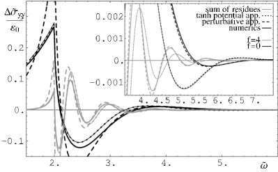
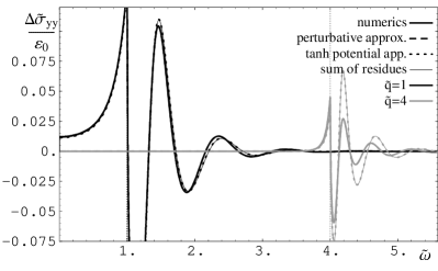
Figure 8: Comparing the conductivity obtained from the numerics, from the approximation (3.78), from the approximation using a $\tanh$ potential (C.129) and from the sum of residues obtained from its poles (C.138). Here we focus on the oscillatory behaviour by plotting $\Delta\tilde{\sigma}_{yy}\equiv{\mbox{Re }}\left(\tilde{\sigma}_{yy}(\tilde{\omega})-\varepsilon_{0}\sqrt{1-\tilde{q}^{2}/\tilde{\omega}^{2}}\right)$, i.e., we subtract off the low temperature limit (3.51). Left: $f\in\{0,4\}$ and $\tilde{q}=2$. Right: $\tilde{q}\in\{2,4\}$ and $f=4$.

4 Quasinormal modes and quasiparticles

In general, the thermal correlators will have poles in the lower half of the complex frequency plane — e.g., see discussion in [41] or [43]. The positions of these poles characterize the energy and lifetime of various excitations in the system. When one of these poles is close to the real axis, the spectral function will show a distinct peak and the corresponding excitation can be interpreted as a quasiparticle. That is, the excitation satisfies Landau’s criterion for a quasiparticle that the lifetime is much greater than the inverse energy. As illustrated in figures 2 and 3, which essentially plot the spectral function, the defect theory is developing metastable quasiparticles in the large $f$ regime. Hence it is of interest to examine the pole structure of the correlators and the spectrum of quasiparticles in the defect conformal field theory. This gives us not only more information on the defect field theory, but also allows us to speculate more on the nature of the defect.

In principle, we could always find the poles in the thermal correlators by simply numerically computing them over the entire complex frequency plane. Of course, such a brute force approach would present an enormously challenging problem at a technical level. However, since the correlators should be meromorphic, we can alternatively try to extract this information by fitting along the real axis, the spectral function derived from an approximate analytical solution of poles and positive powers – an approach similar in spirit to that followed in [43]. To do so, we use the complex “rest frame” frequency ${\tilde{\nu}}=\sqrt{\tilde{\omega}^{2}-\tilde{q}^{2}}$ which maps $[0,\tilde{q}]\rightarrow[i\tilde{q},0]$ and $[\tilde{q},\infty[\rightarrow[0,\infty[$. The motivation to do so is the fact that the resonance pattern is most suitably characterized by $\frac{\tilde{\omega}}{{\tilde{\nu}}}\tilde{\sigma}_{yy}-1$ as a function of ${\tilde{\nu}}$, as shown in figure 9. There we see that even at finite temperature this quantity varies only slowly with varying $\tilde{q}$. Certainly, in the low temperature limit, we expect Lorentz invariance to be restored and then correlators will naturally depend on the combination $\tilde{\omega}^{2}-\tilde{q}^{2}$, as is implicit in (3.51) and (3.61).

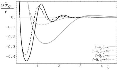
Figure 9: $\frac{\tilde{\omega}}{{\tilde{\nu}}}\tilde{\sigma}_{yy}({\tilde{\nu}})$ for $\tilde{q}\in\{\pi/4,\pi\}$ and $f\in\{0,4\}$. This form of the spectral function is very similar for different values of $\tilde{q}$.

4.1 Finding the Ansatz

The strategy that we will take to find the poles is to take a suitable Ansatz for the location of the $n^{th}$ pole in the complex frequency plane, ${\tilde{\nu}}_{n}=\pm{\tilde{\nu}}_{0}(n)-i{\tilde{\gamma}}_{0}(n)$, and for the corresponding residue, and allow for the parameters to vary slowly. If the Ansatz is good enough, and the parameters vary slowly enough, then we can fit the conductivity resulting from a sequence with constant parameters $({\tilde{\nu}}_{0},{\tilde{\gamma}}_{0})$ to the numerical result using only the data in the region around the $n^{th}$ “resonance”. This data can be parametrized by the amplitude of the resonance around the background and by the gap between the resonances. The resulting parameters $({\tilde{\nu}}_{0}(n),{\tilde{\gamma}}_{0}(n))$ then give the location of the pole ${\tilde{\nu}}_{n}$, and it’s residue.

A suitable guess for the full Ansatz is

$$C_{yy}\,=\,-\varepsilon_{0}\,\sum_{n\geq 1}\frac{1}{\pi}\left(\frac{n({\tilde{\nu}}_{0}+i{\tilde{\gamma}}_{0})^{2}}{{\tilde{\nu}}+n({\tilde{\nu}}_{0}+i{\tilde{\gamma}}_{0})}-({\tilde{\nu}}_{0}+i{\tilde{\gamma}}_{0})\,+\,\frac{n({\tilde{\nu}}_{0}-i{\tilde{\gamma}}_{0})^{2}}{{\tilde{\nu}}-n({\tilde{\nu}}_{0}-i{\tilde{\gamma}}_{0})}+({\tilde{\nu}}_{0}-i{\tilde{\gamma}}_{0})\right)\ ,$$ (4.80)

where the constant terms were introduced to cancel the otherwise divergent behaviour of the series, since the pole terms do not decay for large $n$. The condition that allows us to locally treat the sum as an infinite series with constant $\{{\tilde{\nu}}_{0},{\tilde{\gamma}}_{0}\}$ is now $\partial_{n}\log\{{\tilde{\nu}}_{0}(n),{\tilde{\gamma}}_{0}(n)\}\ll 1$ and $\partial_{n}\log\{{\tilde{\nu}}_{0}(n),{\tilde{\gamma}}_{0}(n)\}\ll\frac{{\tilde{\nu}}_{0}^{2}}{n^{2}{\tilde{\gamma}}_{0}^{2}}$. Rewriting (4.80) in a more suggestive form, we find for ${\tilde{\nu}}\in\mathbb{R}$, i.e., $\tilde{\omega}>\tilde{q}$

$${\mbox{Im }}C_{yy}\,=\,\varepsilon_{0}\,{\mbox{Im }}{\tilde{\nu}}\cot\left(\pi\frac{{\tilde{\nu}}}{{\tilde{\nu}}_{0}+i{\tilde{\gamma}}_{0}}\right)\,=\,\varepsilon_{0}\,{\mbox{Im }}{\tilde{\nu}}\frac{\sin\frac{2\pi{\tilde{\nu}}{\tilde{\nu}}_{0}}{{\tilde{\nu}}_{0}^{2}+{\tilde{\gamma}}_{0}^{2}}\,-\,i\sinh\frac{2\pi{\tilde{\nu}}{\tilde{\gamma}}_{0}}{{\tilde{\nu}}_{0}^{2}+{\tilde{\gamma}}_{0}^{2}}}{\cosh\frac{2\pi{\tilde{\nu}}{\tilde{\gamma}}_{0}}{{\tilde{\nu}}_{0}^{2}+{\tilde{\gamma}}_{0}^{2}}\,-\,\cos\frac{2\pi{\tilde{\nu}}{\tilde{\nu}}_{0}}{{\tilde{\nu}}_{0}^{2}+{\tilde{\gamma}}_{0}^{2}}}\ ,$$ (4.81)

such that we get the conductivity

$$\tilde{\sigma}_{yy}\,=\,\varepsilon_{0}\,\frac{{\tilde{\nu}}}{\tilde{\omega}}\frac{\sinh\frac{2\pi{\tilde{\nu}}{\tilde{\gamma}}_{0}}{{\tilde{\nu}}_{0}^{2}+{\tilde{\gamma}}_{0}^{2}}}{\cosh\frac{2\pi{\tilde{\nu}}{\tilde{\gamma}}_{0}}{{\tilde{\nu}}_{0}^{2}+{\tilde{\gamma}}_{0}^{2}}\,-\,\cos\frac{2\pi{\tilde{\nu}}{\tilde{\nu}}_{0}}{{\tilde{\nu}}_{0}^{2}+{\tilde{\gamma}}_{0}^{2}}}\,,$$ (4.82)

which turns out to be finite at ${\tilde{\nu}}\rightarrow 0$. These exponentially suppressed resonances are characteristically what we expect and we can, in principle, fit the parameters ${\tilde{\nu}}_{0}$ and ${\tilde{\gamma}}_{0}$ to the resonance pattern.

To be more precise however, we need to go back to the original “physical” frequency $\tilde{\omega}$. Keeping the location of the poles and the residue fixed, the sum becomes now

$$C_{yy}=\varepsilon_{0}\,\frac{\tilde{\omega}}{\pi}\log\left(\frac{{\tilde{\nu}}_{0}-i{\tilde{\gamma}}_{0}}{{\tilde{\nu}}_{0}+i{\tilde{\gamma}}_{0}}\right)\ +~{}~{}~{}~{}~{}~{}~{}~{}~{}~{}~{}~{}~{}~{}~{}~{}~{}~{}~{}~{}~{}~{}~{}~{}~{}~{}~{}~{}~{}~{}~{}~{}~{}~{}~{}~{}~{}~{}~{}~{}~{}~{}~{}~{}~{}~{}~{}~{}~{}~{}~{}~{}~{}~{}~{}~{}~{}~{}~{}~{}~{}~{}~{}~{}$$ (4.83)

$$\varepsilon_{0}\,\sum_{n\geq 1}\frac{1}{\pi}\left(\frac{n({\tilde{\nu}}_{0}-i{\tilde{\gamma}}_{0})}{\big{(}\tilde{q}^{2}+n^{2}(-{\tilde{\nu}}_{0}+i{\tilde{\gamma}}_{0})^{2}\big{)}^{1/2}}\left(\frac{n({\tilde{\nu}}_{0}-i{\tilde{\gamma}}_{0})^{2}}{\tilde{\omega}-\big{(}\tilde{q}^{2}+n^{2}({\tilde{\nu}}_{0}-i{\tilde{\gamma}}_{0})^{2}\big{)}^{1/2}}+\frac{n({\tilde{\nu}}_{0}-i{\tilde{\gamma}}_{0})^{2}}{\big{(}\tilde{q}^{2}+n^{2}({\tilde{\nu}}_{0}-i{\tilde{\gamma}}_{0})^{2}\big{)}^{1/2}}\right)\right.$$

$$\left.-\,\frac{n({\tilde{\nu}}_{0}+i{\tilde{\gamma}}_{0})}{\big{(}\tilde{q}^{2}+n^{2}({\tilde{\nu}}_{0}+i{\tilde{\gamma}}_{0})^{2}\big{)}^{1/2}}\left(\frac{n({\tilde{\nu}}_{0}+i{\tilde{\gamma}}_{0})^{2}}{\tilde{\omega}+\big{(}\tilde{q}^{2}+n^{2}({\tilde{\nu}}_{0}+i{\tilde{\gamma}}_{0})^{2}\big{)}^{1/2}}-\frac{n({\tilde{\nu}}_{0}+i{\tilde{\gamma}}_{0})^{2}}{\big{(}\tilde{q}^{2}+n^{2}({\tilde{\nu}}_{0}+i{\tilde{\gamma}}_{0})^{2}\big{)}^{1/2}}\right)\right),$$

where the term $\frac{\tilde{\omega}}{\pi}\log\frac{{\tilde{\nu}}_{0}-i{\tilde{\gamma}}_{0}}{{\tilde{\nu}}_{0}+i{\tilde{\gamma}}_{0}}$ cancels the unphysical negative DC conductivity in the $\tilde{q}\gg{\tilde{\nu}}_{0},{\tilde{\gamma}}_{0}$ limit that would arise otherwise. Note there is still a logarithmic divergence in the real part, that we are not interested in. This sequence does not sum to any known analytic expression, but the integral approximation can be computed straightforwardly analytically, such that in order to eventually study the sequence numerically, we will only sum the first few hundred poles and add a small “background” contribution from the rest of the poles using the integral.

Following the same considerations, we also find an Ansatz for the longitudinal correlator,

$$C_{xx} = \varepsilon_{0}\,\sum_{n\geq 1}\frac{1}{(n\!-\!\frac{1}{2})\pi}\left(\frac{(n\!-\!\frac{1}{2})({\tilde{\nu}}_{0}-i{\tilde{\gamma}}_{0})}{\big{(}\tilde{q}^{2}+\big{(}n\!-\!\frac{1}{2}\big{)}^{2}({\tilde{\nu}}_{0}-i{\tilde{\gamma}}_{0})^{2}\big{)}^{1/2}}\ \frac{1}{\tilde{\omega}-\big{(}\tilde{q}^{2}+\big{(}n\!-\!\frac{1}{2}\big{)}^{2}({\tilde{\nu}}_{0}-i{\tilde{\gamma}}_{0})^{2}\big{)}^{1/2}}\right.$$ (4.84)

$$\quad-\left.\frac{(n\!-\!\frac{1}{2})({\tilde{\nu}}_{0}+i{\tilde{\gamma}}_{0})}{\big{(}\tilde{q}^{2}+\big{(}n\!-\!\frac{1}{2}\big{)}^{2}({\tilde{\nu}}_{0}+i{\tilde{\gamma}}_{0})^{2}\big{)}^{1/2}}\ \frac{1}{\tilde{\omega}+\big{(}\tilde{q}^{2}+\big{(}n\!-\!\frac{1}{2}\big{)}^{2}({\tilde{\nu}}_{0}+i{\tilde{\gamma}}_{0})^{2}\big{)}^{1/2}}\right)\ ,$$

which converges and needs no regularization or terms with positive powers of $\tilde{\omega}$. In terms of ${\tilde{\nu}}$, the poles are located at $(n-1/2)(\pm{\tilde{\nu}}_{0}-i{\tilde{\gamma}}_{0})$, with residues $\frac{1}{n-1/2}$, as we expect by (3.59) from the ansatz for $C_{yy}$.

In order to finally obtain the location of the poles and their residue, we split the spectral function at the minima into segments around each maximum and simply fit them to our Ansatz giving us a set of parameters that we attribute to the local properties of the sequence at the most nearby pole, as described in the beginning of the section. We obtain both ${\tilde{\nu}}_{0}$ and ${\tilde{\gamma}}_{0}$ and an overall factor $(1+\epsilon_{\mathscr{R}})$ (or $(1+\epsilon_{\mathscr{R}})^{\star}$ on the negative branch) for the residues. The latter is needed because the resonance pattern is exponentially suppressed already for reasonably small ${\tilde{\nu}}\gtrsim\pi$, such that the background of the fitted sequence needs to be adjusted to in precise agreement with the background of the data, in order to extract the relevant information which is contained in the resonances. As it turns out that $|\epsilon_{\mathscr{R}}|\ll 1$, we will not comment about its value for the rest of the paper, because it is irrelevant for both the quantitative and the qualitative discussions. In principle, one can introduce more parameters, such as an overall shift in the frequency, but this would not improve the results, since in practice, it simply introduces extra degeneracy in parametrizing the fit.

4.2 Quasiparticles from the collisionless regime

Given the Ansatz for the transverse and longitudinal correlators above, we will now discuss the results for determining the positions of the poles. The results are only displayed for Re ${\tilde{\nu}}>0$ but as shown in (4.80), there is a corresponding set of poles with Re ${\tilde{\nu}}<0$. In this section, we focus on the collisionless or short-wavelength regime with $\tilde{\omega}\gg 1$ and $\tilde{q}\mathrel{\raisebox{-2.58334pt}{$\stackrel{{\scriptstyle\textstyle>}}{{\sim}}$}}1$.

As a first test, we compare the fitted location of the poles to their exact location for the $\tanh$ potential in appendix C.2. We expect that this gives us a good estimate for the quality of the fit for the actual spectral functions. Some typical results are shown in the first plot of figure 10. We find that for $f=0$, the fit is very poor, with the $\tilde{q}=\pi/4$ result being worse than the $\tilde{q}=\pi$ case, and there is a small deviation for $f=4$ at large $\tilde{\omega}$, again with a slightly better fit for larger $\tilde{q}$. Apart from that, i.e., for large $f$ or large $\tilde{q}$ and small $\tilde{\omega}$, the fit is very good. This is just what we would have expected from our conditions for the validity of the Ansatz as smaller $\tilde{q}$ imply more rapidly varying ${\tilde{\nu}}_{0},{\tilde{\gamma}}_{0}$ at least for the first few poles and both small $f$ and $\tilde{q}$ and large $\tilde{\omega}$ move the poles further away from the real axis. Furthermore, for large $\tilde{\omega}$, the amplitude of the resonance pattern becomes quickly suppressed and so it is subject to systematic deviations and noise.

Now, let us look at the qualitative behaviour. We see that, as anticipated with the Ansatz, the poles lie roughly equally spaced on a straight line, i.e., they are resonances in a region of fixed width with fixed “mass” to inverse lifetime ratio. With increasing $f$, both the separation of the poles and the slope of the line of poles decreases, i.e., the poles are moving closer to the real axis. Of course, these changes are reflected by the appearance of distinct peaks in the previous plots of conductivity at large $f$. This behaviour is roughly independent of $\tilde{q}$, and there is an overall shift depending on $\tilde{q}$, that is larger for smaller values of $f$. One might expect both the decreasing energy gap and the increasing mass to width ratio since the length scale due to the width of the defect increases and the shape of the step in the potential is approximately fixed. The deviation of the poles from a straight line is stronger for large $\tilde{q}$ and reflects the fact that the shallow potential at small $\tilde{q}$ is fully probed at small ${\tilde{\nu}}$, whereas at large $\tilde{q}$, the resonances at small ${\tilde{\nu}}$ are only sensitive to the details of the top of the potential, and only probe the steeper regions at higher $n$. This effect is obviously more visible at large $f$ because of the closer spacing of the resonances. We also see that the poles of the transverse correlator lie roughly half-way between the poles of the longitudinal correlator, as anticipated in (3.59). Comparing the various approximations to the location of the poles of the actual spectral function, we see the behaviour that we saw in figure 8 encoded in a different way. Here, we see the shift of the poles of the $\tanh$ potential that is more significant for larger $\tilde{q}$.

As an aside, let us briefly return to the cuts that appeared in the the transverse and longitudinal conductivities, in (3.51) and (3.61), with the limit $T\to 0$. Given the present analysis, it is natural to conclude that this cut arises through an accumulation of poles near $\tilde{\omega}\sim\tilde{q}$. Assuming the locations of the poles in the ${\tilde{\nu}}$ plane, ${\tilde{\nu}}_{n}$, to be roughly independent of $\tilde{q}$, we find that for $\tilde{q}\gg 1$ we get $\tilde{\omega}_{n}=\sqrt{{\tilde{\nu}}_{n}^{2}+\tilde{q}^{2}}\sim\tilde{q}+{\tilde{\nu}}_{n}^{2}/\tilde{q}$. This then leads to an infinite number of poles accumulating near $\tilde{\omega}=\tilde{q}$ as $T\to 0$ and resulting in a cut.

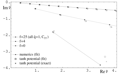
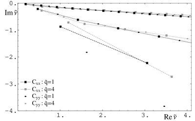
Figure 10: Left: Comparing the exact location of the poles of the transverse correlator to the fit, using the approximate $\tanh$-potential of appendix C, at values $f\in\{0,4,25\}$ and $\tilde{q}=1$. Right: Comparing the poles of the transverse correlator with the ones of the longitudinal correlator at $f\in\{0,4,25\}$ and $\tilde{q}\in\{1,4\}$. The lines are only shown to guide the eye as to which poles correspond to the same values of $f,\tilde{q}$.

While the Ansatz (4.80) fixes the poles along a straight line with a fixed spacing, i.e., ${\tilde{\nu}}=n({\tilde{\nu}}_{0}-i{\tilde{\gamma}}_{0})$ in the Re ${\tilde{\nu}}>0$ region, we fit the parameters locally to each peak of the spectral function and so the fitted poles deviate slightly from this simple Ansatz. Keeping in mind the limitations, let us try to extract some quantitative information on these deviations. In particular, at large $n$, the poles approach a straight line of the form ${\tilde{\nu}}_{n}=\delta{\tilde{\nu}}+i\delta\gamma+n({\tilde{\nu}}_{0}+i{\tilde{\gamma}}_{0})$ (${\tilde{\nu}}_{n}=\delta{\tilde{\nu}}+i\delta\gamma+(n-1/2)({\tilde{\nu}}_{0}+i{\tilde{\gamma}}_{0})$ in the longitudinal case). To extract this information, we use different techniques in different regimes, which we outline to forewarn the reader about the validity of the results. For large $f$, where we have at least the first 5 well-fitted poles, we ignore the first 0-3 poles, leaving us at least 5 poles, such that we can fit the asymptotic lines plus a decaying exponential to ${\mbox{Re }}{\tilde{\nu}}_{n}$ and ${\mbox{Im }}{\tilde{\nu}}_{n}$ and still get information about the accuracy. For some cases, the exponential fit fails, and we resort to fitting a straight line and estimate the accuracy from the second derivative in the location of the poles.

The assumption of an exponential deviation from a straight line may seem somewhat arbitrary, but it turns out to be the right choice, as it is the only natural candidate whose results are independent within errors from the particular choice of the number of poles used for the regression. The location of the poles from the $\tanh$ potential, for example, contains by this criterion an $\mathscr{o}(\ln n)$ term as expected from (C.132).

In the borderline case, where there are 4 poles, we extract the uncertainties by fitting the last 3 poles to the asymptotic line with the deviation estimated by the fit with 4 points. For 3 poles only, we still get a rough estimate for the asymptotic limit (from the last 2 points) and for the accuracy by including the first point. For $f=0$, we always find only the first two poles, so we can give only an order of magnitude guess for the rest of the sequence. Finally, we estimate the uncertainties from the errors in the fit of the sequence of poles and from the deviation of the estimated location of poles to their exact location in the case of the $\tanh$ potential. We use the latter also to add a shift to try to correct for systematic errors in the fit of the Ansatz (4.83, 4.84) to the numerical data. We are somewhat sloppy with the uncertainties in the sense that we do not distinguish between random and systematic errors. So we assume that the accuracy of the fits is limited by systematic uncertainties in the convergence towards the asymptotic straight line, which may result in a slight overestimating of uncertainties in the averaged data that we present below. As expected, the results from the transverse and longitudinal poles are identical within the errors and so we average over them.

Let us now examine some of the results of our fitting in figure 11. In the first two plots, we show results for the energy gap between the quasinormal modes, ${\tilde{\nu}}_{0}$. In particular for large $f$, we see that the asymptotic behaviour of $\pi/{\tilde{\nu}}_{0}$ matches a simple straight-line fit: $\pi/{\tilde{\nu}}_{0}=c_{1}\sqrt{f}+c_{0}$ with $c_{1}\simeq 1.821$ and $c_{0}\simeq-0.539$. In the first plot, this behaviour seems to match well with the asymptotic behaviour of $\pi T/(2T_{eff})$ and $\pi D(f)T$. Note, however, that the second plot shows that upon closer examination, the deviation between $\pi/{\tilde{\nu}}_{0}$ and the curves set by these scales in the large $f$ regime seems to be beyond the errors expected for our numerical fit to ${\tilde{\nu}}_{0}$. Note that large $f$ behaviour in (3.2.1) gives $\pi T/(2T_{eff})\simeq 1.854\sqrt{f}-0.690$, while (A.110) yields $\pi DT\simeq 1.854\sqrt{f}-1$. The asymptotic behaviours for these quantities have precisely the same slope and the difference is in the constant term (and the subleading $1/\sqrt{f}$ terms), as can be seen in figure 11. This slope is only a fair match for that found in our straight-line fit. We expect that this is because of subleading $1/\sqrt{f}$ terms and that we would see better convergence at larger values of $f$. In any event, it seems then that ${\tilde{\nu}}_{0}$ is closely related to other characteristic scales in the defect theory. Note that here since ${\tilde{\nu}}_{0}$ appears to be independent of $\tilde{q}$ within the errors (see figure 12), the data in figure 11 is averaged over $\tilde{q}\in{\pi/2,\pi,2\pi}$.

We also show the overall shift $\delta{\tilde{\gamma}}$ and the ratio ${\tilde{\gamma}}_{0}/{\tilde{\nu}}_{0}$ separately in figure 11 for the cases $\tilde{q}\in{\pi/2,\pi,2\pi}$. In each case, these parameters show a $1/\sqrt{f}$ falloff for large $f$. In particular, this means that the width ${\tilde{\gamma}}_{0}$ is falling as $1/f$ and so we see the origin of the quasiparticle peaks in the spectral curves. In each plot, we also show $\pi T/(2T_{eff})$ for each case and see there is good agreement within the estimated errors of the numerical results. This is just what we expect, since the detailed shape of the step in the effective Schrödinger potential and hence the ratio between the two modes in the asymptotic region of the potential, is to a good approximation independent of $f$. The slowly varying part of this ratio gives rise to the finite shift and the exponential suppression factor gives rise to ${\tilde{\gamma}}_{0}/{\tilde{\nu}}_{0}$, which are in the limit of large $\tilde{\omega}$ proportional to the inverse of the width of the asymptotic region of the potential. This can be more easily seen from the expressions in appendix C.2. From the boundary point of view, it comes at no surprise that the overall shift of the poles is proportional to the overall energy scale, and that the quasiparticle excitations become more stable with increasing $f$, which is proportional to the width of the potential step. One could make a similar plot of $\delta{\tilde{\nu}}$ but we do not show the results here. While on the whole the trends appear similar to those for $\delta{\tilde{\gamma}}$, the values are typically smaller by a factor of roughly 2 while the relative errors are larger by a similar factor. Hence at least for the smaller values of $\tilde{q}$, the results are consistent with zero shift.

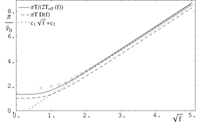
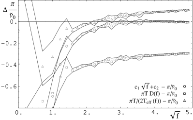
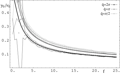
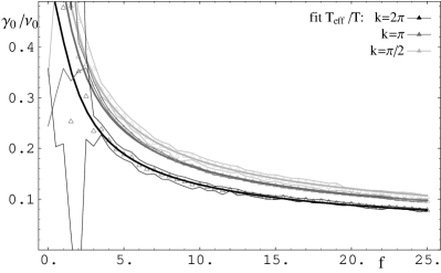
Figure 11: Top left: The energy gap between resonances ${\tilde{\nu}}_{0}$ presented as $\pi/{\tilde{\nu}}_{0}$. The asymptotic $\sqrt{f}$ behaviour is fit is several ways. Top right: The difference between the previous fits and the numerical results for $\pi/{\tilde{\nu}}_{0}$. The data in the top two plots is averaged over $\tilde{q}\in{\pi/2,\pi,2\pi}$. Bottom left: The “mass to width” ratio ${\tilde{\gamma}}_{0}/{\tilde{\nu}}_{0}$ for the sequence of poles for several values of $\tilde{q}$. Bottom right: The $f$-dependence of the overall shift of the poles $\delta{\tilde{\gamma}}$. The points are the average numerical data and the narrow lines indicate the $1\sigma$ uncertainties, which includes both random and systematic errors.

Now let us turn to the $\tilde{q}$ dependence of the quasinormal modes. Because of the good agreement of the $f$ dependence with $T_{eff}/T$, we improve the accuracy of our results by taking a (weighted) average over the suitably scaled values of the characteristic quantities for $f\in\{9,16,25,36\}$. In figure 12, we show the $\tilde{q}$ dependence of the same quantities as in figure 11. First, we see that ${\tilde{\nu}}_{0}$, which is supposed to depend only on the width of the potential, is within the uncertainties independent of $\tilde{q}$. Any change in $\tilde{q}$ however scales only the height of the potential step.

From the results in appendix C.2, we would expect that varying $\tilde{q}$ changes only the overall shift of the poles, but we know already that the full result has fundamentally different characteristics coming from the shape of the potential step because of the absence of a significant $\mathscr{o}(\ln n)$ term. In general, however, ${\tilde{\nu}}_{0}$ should not change significantly, since we consider here only $f\geq 9$, so the potential is already so wide that small details of probing the potential step should not change the the quasinormal modes too much. Both the shift, and the deviation from the linear Ansatz conspire to give us both the right “low temperature background” with approximately symmetric oscillations around it as in figure 9. From the fact that this behaviour resembles that in the resulting conductivity from (4.81), one should assume that there are small shifts and deviations for small $\tilde{q}$. One also expects the shift to grow not faster than $\propto\ln\tilde{q}$, provided that the ratio of the two modes in the asymptotic region depends at most on some power of the height of the step in the potential.

In figure 12, we find roughly this behaviour of the shift, with small $\delta{\tilde{\nu}},{\tilde{\gamma}}$ at small $\tilde{q}$ and an indication of some converging or slowly growing behaviour at large $\tilde{q}$. We also find a small drop in ${\tilde{\gamma}}_{0}/{\tilde{\nu}}_{0}$ with some converging behaviour at large $\tilde{q}$. In principle, we could try to use this information to try to reverse engineer the calculations in appendix C.2, i.e., to reconstruct the ratio of the incoming and outgoing modes. For example, the absence of a significant $\mathscr{o}(\ln n)$ term tells us that there is no significant ${\tilde{\nu}}$ dependence, the approximately constant (in $f$) ratio $\delta{\tilde{\nu}}/\delta{\tilde{\gamma}}$ shows us that the ratio of the modes has a complex phase (and also its value) but there is nothing really interesting to learn from this. A somewhat interesting point though is that the change in ${\tilde{\gamma}}_{0}/{\tilde{\nu}}_{0}$ tells us that at small $\tilde{q}$, the potential “appears smoother” than at large $\tilde{q}$.

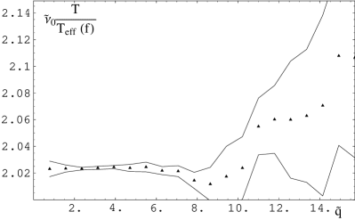
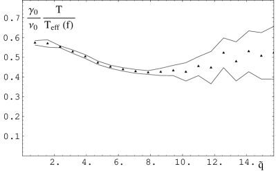
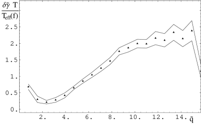
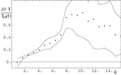
Figure 12: Average over quantities appropriately scaled with $T_{eff}(f)/T$ for $f\in\{9,16,25,36\}$: Top left: (In)dependence of ${\tilde{\nu}}_{0}$ on $\tilde{q}$. Top right: ${\tilde{\gamma}}_{0}/{\tilde{\nu}}_{0}$. Bottom: The complex shift $\delta{\tilde{\nu}}$ and $\delta{\tilde{\gamma}}$.

4.3 Poles in the hydrodynamic regime

In this section, we focus on the hydrodynamic regime where $\tilde{\omega},\tilde{q}\ll 1$. In this regime, the diffusion pole (3.62) dominates the structure of the correlators. One might wonder, why we have not included the diffusion pole into the sum for $C_{yy}$, as in (4.80). As we will show below, this is because the diffusion pole disappears at a critical value of the wave-number, $\tilde{q}_{c}$, which is below the values of $\tilde{q}$ that we have considered to this point. Below $\tilde{q}_{c}$ there are two poles on the imaginary axis in the $\tilde{\omega}$ plane, one of them being the diffusion pole, and the other one at larger absolute imaginary values of $\tilde{\omega}$, which decreases slowly as $\tilde{q}$ grows, as shown in figure 13. While the diffusion pole is in perfect agreement with what we expected, the second pole, corresponding to rapid (i.e., on thermal scales) decay of long-range modes, is somewhat puzzling. In particular, it has a non-trivial $f$ dependence at small values of $\tilde{q}$. It seems that for large $f$, the lifetime of those modes is not anymore proportional to the length scale of the defect, but increases less rapidly.

At $\tilde{q}_{c}$, there is a branch cut, and the poles move away from the imaginary axis out into the complex plane to turn into the first quasiparticle poles, i.e., the $n=1$ poles in (4.80). Hence at this point, the transport changes from the collision dominated phase to the collisionless phase. This is a good example of the interplay between various length scales. We can interpret this on the one hand as the height of the effective potential being smaller or larger than the inverse length scale of the defect (and hence the effective temperature) and on the other hand as separating between between modes smaller and larger than the size of the defect. From a hydrodynamic viewpoint, however this branch cut gives us approximately the mean free path, which is in strongly coupled systems proportional to, and of the same order as, the temperature scale, and we see an approximate scaling of $\tilde{q}_{c}$ with the effective temperature.

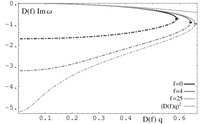
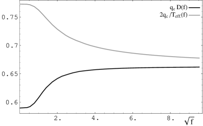
Figure 13: Left: The location of the poles on the imaginary axis below $q_{c}$, rescaled by the diffusion constant. The dashed line is what one expects for the diffusion pole. Right: The critical values $q_{c}$ at which the purely dissipative poles disappear, multiplied with several length scales.

On the right in figure 13, we compare $\tilde{q}_{c}$ with the various length scales in the problem, as we did before for the spacing of the quasiparticle masses in figure 11. Since we are in the completely opposite regime in terms of length scales of the perturbations, it is no surprise that there is significant disagreement between the scaling of $\tilde{q}_{c}$ and ${\tilde{\nu}}_{0}$, but the disagreement is surprisingly small. In addition to the opposite limit of the size of the perturbations, the data in figure 11 contains only frequencies, which one can interpret as being related directly to the width of the defect, whereas here we consider the $f$-dependence of relevant values of $\tilde{q}$, which measure scales along the defect. Overall, it seems that in the limit of large $f$, $\tilde{q}_{c}\simeq 2/(3\,D)$ or $\tilde{q}_{c}\simeq 4T_{eff}/3$. The relative factor between these two expressions is not surprising given that, in the previous section, we noted that $D=2/T_{eff}$ as $f\to\infty$. Further, given our previous expressions for $D$ and $T_{eff}$, we note that $\tilde{q}_{c}\propto T/\sqrt{f}$ for large $f$, i.e., $\tilde{q}_{c}$ decreases as $f$ grows. Then as the plot shows, up to an overall numerical factor, most features of the $f$-dependence of $\tilde{q}_{c}$ can be related to either of these other physical scales.

In principle, the decreasing residue of the poles with increasing $n$ allows us to track the location of the first few poles of the longitudinal correlator even further, directly by fitting a sequence of Lorentzians, but we will not bother about such a detailed discussion of the hydrodynamic regime in this paper. It is interesting to see however, how the small-$\tilde{q}$ limit of the shift $\delta{\tilde{\nu}}+i\delta{\tilde{\gamma}}$ shown in figure 12 qualitatively agrees with a shift towards the bifurcation point.

It is interesting to note that this pairing of the diffusion pole with a fast dissipative mode was also recently found in the quasinormal mode spectrum of black holes in AdS₄ [44]. However, an infinite number of pairs of poles were identified there, appearing along the imaginary axis. In that case, the critical wave-number at which the higher pairs meet at smaller and move off into the complex plane decreases for pairs higher up along the imaginary axis. We looked for similar higher dissipative modes in the present framework but it seems that the diffusion mode and its partner are the only modes appearing on the imaginary frequency axis.

5 Electromagnetic duality and perturbative corrections

At the outset of our analysis, we set $M_{\textrm{\tiny q}}=0$ to maintain conformal invariance in the defect system. In the brane construction, this means the internal geometry is fixed and the low energy effective action on the effective four-dimensional brane reduces to Maxwell theory (3.31) with a fixed coupling (independent of the radius). Hence resulting equations of motion are invariant under electromagnetic duality, which has interesting implications for the transport coefficients, as emphasized in [5].

Given the Maxwell action (3.31), the gauge field equations can be expressed as

$$\nabla^{\mu}F_{\mu\nu}=0\,,\qquad\nabla^{\mu}\widetilde{F}_{\mu\nu}=0\qquad{\rm with}\ \widetilde{F}_{\mu\nu}=\frac{1}{2}\,\varepsilon_{\mu\nu\rho\sigma}F^{\rho\sigma}\ .$$ (5.85)

Hence we have electromagnetic duality with $F_{\mu\nu}$ and $\widetilde{F}_{\mu\nu}$ satisfying the same equations of motion. Implicitly, we used this duality in deriving the relation between the transverse and longitudinal correlators (3.59), i.e., the key step was demonstrating the $A_{\tilde{t}}$ and $A_{\tilde{y}}$ equations, (3.45) and (3.47), could be put in the same form. As in [5], this result (3.59) subsequently restricts the transport coefficients to satisfy

$$\Pi^{T}(\tilde{\omega},\tilde{q})\,\Pi^{L}(\tilde{\omega},\tilde{q})=-\varepsilon_{0}^{2}(\tilde{\omega}^{2}-\tilde{q}^{2})\ .$$ (5.86)

Since with $\tilde{q}=0$, we have $\Pi^{T}(\tilde{\omega},0)=\Pi^{L}(\tilde{\omega},0)$, it follows that:

$${\tilde{\sigma}}(\tilde{\omega})=i\frac{\Pi(\tilde{\omega},0)}{\tilde{\omega}}=\varepsilon_{0}=\pi\,D\,T\,\varepsilon\,~{}~{}~{}\mathrm{or}~{}~{}~{}\sigma(\omega)=D\,\varepsilon\,.$$ (5.87)

That is, $\sigma(\omega)$ is independent of frequency and temperature. One can show that this remarkable result is consistent with the Einstein relation, as noted already in [5].

However, as for any low energy action in string theory, we must expect that there are higher derivative interactions correcting the Maxwell action (3.31). In fact, the action (2.4) implicitly captures an infinite set of these stringy corrections, as would be illustrated if we expanded the DBI term in powers of $F$. This expansion would also demonstrate that these higher order terms are suppressed by factors of $\alpha^{\prime}=\ell_{\textrm{\tiny s}}^{2}$. In terms of the dual CFT, the contributions of these $\alpha^{\prime}$ interactions will provide corrections to the leading supergravity results for a finite ’t Hooft coupling. However, none of the higher order terms coming from the DBI action will modify the two-point correlators in the planar limit, i.e., in the large $N_{\textrm{\tiny c}}$ limit, because these interactions all involve higher powers of the field strength. One must keep in mind though that, as already alluded to in section 2.2, the DBI action does not capture all of the higher dimension stringy interactions. The full low-energy action includes additional terms involving derivatives of the gauge field strength [45, 46], as well as higher derivative couplings to the bulk fields, e.g., curvature terms [47, 48]. In principle, any such interaction, which is quadratic in $F$, has the potential to make finite $\lambda$ corrections to the correlators which we have studied above.

In appendix B, we identified a particular higher derivative term which makes a quadratic correction (B.112) to the four-dimensional low energy action. This term makes the leading correction to the correlators, at least when the internal flux is nonvanishing. Including this term, the vector equations of motion become

$$\nabla^{\mu}F_{\mu\nu}=\xi\,L^{2}\,\nabla^{\mu}\Box F_{\mu\nu}\,,\qquad\nabla^{\mu}\widetilde{F}_{\mu\nu}=0\qquad{\rm with}\ \xi=\frac{\zeta(3)}{2\pi\sqrt{\lambda}}\frac{f^{2}}{\sqrt{1+f^{2}}}\ .$$ (5.88)

We can recognize the higher derivative term as a string correction by recalling that $L^{2}/\sqrt{\lambda}=\ell_{\textrm{\tiny s}}^{2}$. Clearly these equations are no longer invariant under the replacement: $F_{\mu\nu}\rightarrow\widetilde{F}_{\mu\nu}$. One could attempt an $\alpha^{\prime}$-corrected electromagnetic duality by defining $\widetilde{X}_{\mu\nu}=\left(1-\xi\,L^{2}\Box\right)F_{\mu\nu}$. Formally treating $\xi$ as a small expansion parameter, one can rewrite (5.88) as

$$\nabla^{\mu}X_{\mu\nu}=-\xi\,L^{2}\,\nabla^{\mu}\Box X_{\mu\nu}\,,\qquad\nabla^{\mu}\widetilde{X}_{\mu\nu}=0\ .$$ (5.89)

Hence an exchange $F_{\mu\nu}\rightarrow X_{\mu\nu}$ does not quite leave the equations of motion invariant either, i.e., the sign of the $\xi$ term changes between (5.88) and (5.89). This then confirms the initial intuition that the $\alpha^{\prime}$-corrected low energy theory describing the four-dimensional dynamics of the vector field is no longer invariant under electromagnetic duality. Hence we can longer expect (5.86) and (5.87) to apply when finite $\lambda$ corrections are taken into account for the defect CFT.

In the following, we examine in more detail the effect of this leading finite $\lambda$ correction. For simplicity, we focus on the modifications to the transverse conductivity ${\tilde{\sigma}}_{yy}$. Here we simply present the results of our numerical calculations. The preliminary analysis determining the analytic form of the transverse correlator is given in appendix B. There are two distinct contributions to the modification of the correlator. First, since the bulk action contains an additional term, there are new surface terms (B.118) which must be evaluated in the holographic calculation. Remarkably, as described in the appendix, the net effect of this contribution is to shift the permittivity

$$\varepsilon_{0}\to\varepsilon_{0}\left(1-\frac{1}{\sqrt{\lambda}}\frac{f^{2}\,\zeta(3)}{\pi(1+f^{2})^{3/2}}\right)=\varepsilon_{0}\left(1-\frac{2\,\xi}{1+f^{2}}\right)\,.$$ (5.90)

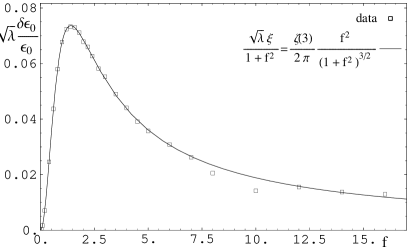
Figure 14: The modification of $\varepsilon_{0}\equiv{\tilde{\sigma}}(\tilde{\omega}\rightarrow\infty)$ as a function of $f$ from the $1/\sqrt{\lambda}$ corrections.

The second modification of the correlator arises because the bulk equations of motion have been corrected, as in (5.88). Hence the solutions for the vector are modified and this change of the solution alone leads to changes in the correlator coming from the leading supergravity expression (3.41). Now, we have some ambiguity in how we might define $\varepsilon_{0}$ in the theory with finite-$\lambda$ corrections. Recall that this quantity originally appeared in (3.40) but above was simply related to the conductivity (5.87) found in the infinite $\lambda$ limit. Hence a convenient choice, which we adopt at finite $\lambda$, is: $\varepsilon_{0}\equiv\ {\tilde{\sigma}}(\tilde{\omega}\rightarrow\infty)$. Then our numerical results indicate that this second finite-$\lambda$ correction also shifts $\varepsilon_{0}$ precisely as in (5.90) except for a factor of $-3/2$. The total shift is shown in figure 14 and the result seems to match precisely $-1/2$ times the shift given in (5.90).

Given that the invariance under electromagnetic duality is lost at finite $\lambda$, the frequency independence of the conductivity ${\tilde{\sigma}}(\tilde{\omega})={\tilde{\sigma}}_{yy}(\tilde{\omega},\tilde{q}=0)$ found in (5.87) is also lost as shown in figure 16. Note that here we are plotting the change arising from the inclusion of the finite $\lambda$ corrections, i.e., $\delta{\tilde{\sigma}}(\tilde{\omega})={\tilde{\sigma}}(\tilde{\omega})-\varepsilon_{0}$ where our subtraction includes the finite-$\lambda$ correction to $\varepsilon_{0}$, as described above. Note that in the figure, the factor $1/\xi\propto\frac{\sqrt{1+f^{2}}}{f^{2}}$ is included to cancel the $f$ dependence coming from the factor in front of the higher order term in (B.114). While the resulting conductivity shows an oscillatory behaviour, we note that the DC conductivity, i.e., at $\tilde{\omega}=0$, is generally smaller than at high frequencies, i.e., for $\tilde{\omega}\rightarrow\infty$. The net difference is plotted in figure 16, as a function of $f$. As shown, the numerical results are very well fit with a simple analytic form proportional to $f^{2}/(1+f^{2})$. Note that the first few points in this plot (including where the difference becomes positive) are not reliable, because of the high sensitivity to errors in $\delta\varepsilon_{0}$, which was only computed approximately in a numerical calculation.

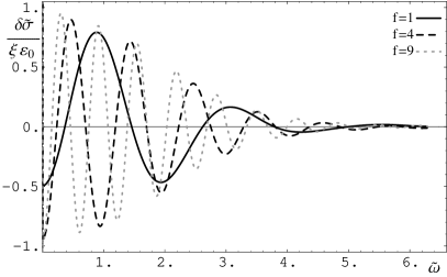
Figure 15: The finite-$\lambda$ correction to the conductivity $\delta{\tilde{\sigma}}(\tilde{\omega})$ for various values of $f$.

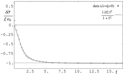
Figure 16: ${\tilde{\sigma}}(\tilde{\omega}=0)-{\tilde{\sigma}}(\tilde{\omega}\rightarrow\infty)$, the change in conductivity from $\tilde{\omega}=0$ to $\tilde{\omega}\rightarrow\infty$ at finite $\lambda$.

One of the interesting features that figure 16 seems to exhibit is that the oscillations of ${\tilde{\sigma}}(\tilde{\omega})/(\xi\varepsilon_{0})$ for various values of $f$ are all contained within some universal envelope, that is decaying with $\tilde{\omega}$. In fact, this same envelope also applies for the conductivity at finite values of $\tilde{q}$, as illustrated in figure 18. In this figure, we are showing ${\delta{\tilde{\sigma}}_{yy}}/(\varepsilon_{0}\xi)$ for $f\in\{1,4,9,16\}$ and $\tilde{q}\in\{0,\pi/4,\pi/2,\pi,2\pi\}$, where $\delta{\tilde{\sigma}}_{yy}\equiv{\tilde{\sigma}}_{yy}(\tilde{\omega},\tilde{q})-{\tilde{\sigma}}_{yy}(\tilde{\omega}\rightarrow\infty,\tilde{q})$. Again, the factor $1/\xi$ is included in the figure to cancel the $f$ dependence explicitly appearing in the higher order term in (B.114). In particular, we see here that the envelope appears to be independent of $\tilde{q}$. However, as shown in figure 18, for sufficiently small $f$ ($f=1/4$ in the figure), there exists a critical value of $\tilde{q}$, above which the conductivity is no longer bounded by this universal envelope. Note that for the same values of $f$, the curves below the critical value of $\tilde{q}$ are still bounded by the envelope. However, note that both $\xi,\varepsilon_{0}\,\propto f$ for large $f$ and so the amplitude of oscillations in ${\tilde{\sigma}}(\tilde{\omega})$ alone is actually growing with $f$.

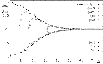
Figure 17: The extrema of $\frac{1}{\varepsilon_{0}\xi}\delta{\tilde{\sigma}}_{yy}$ for $\tilde{q}\in\{0,\pi/4,\pi/2,\pi,2\pi\}$ and “large” $f\in\{4,9,16\}$. We see that all the curves are approximately bound by some universal envelope function, that decays exponentially in $\tilde{\omega}$.

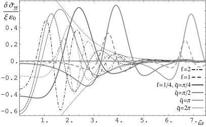
Figure 18: $\frac{1}{\varepsilon_{0}\xi}\delta{\tilde{\sigma}}_{yy}$ for $\tilde{q}\in\{\pi/4,\pi/2,\pi\}$ and $f\in\{1/4,1\}$. For $f=1/4$ and sufficiently large $\tilde{q}$, the conductivity is not bounded by the universal envelope (shown in thin dots).

At finite $\tilde{q}$, the leading order result (for infinite $\lambda$ and $N_{\textrm{\tiny c}}$) for ${\tilde{\sigma}}_{yy}$ also exhibited similar damped oscillations which were confined within a certain envelope, as discussed in 3.2.2. Comparing this previous envelope with that for $\delta{\tilde{\sigma}}_{yy}$ (for large $f\gtrsim 2$), we see that the previous one does not depend only on $\tilde{\omega}$, in contrast to the behaviour found above. The exponential decay of the amplitude at large $\tilde{\omega}$ is also slower than here than with the envelope for the leading infinite-$\lambda$ result. This would imply that the finite-$\lambda$ corrections become more and more significant at large $\tilde{\omega}$, while they become less significant with increasing $\tilde{q}$.

The “frequency” of the oscillations is approximately the same for the leading term and the finite-$\lambda$ correction. Figure 19 shows this in more detail by plotting $\frac{\sqrt{\lambda}}{\varepsilon_{0}}\delta{\tilde{\sigma}}_{yy}$ in terms of $\sqrt{\tilde{\omega}^{2}-\tilde{q}^{2}}$ and also for comparison the oscillations of the infinite-$\lambda$ or “zero’th order” result.

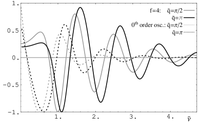
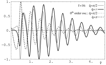
Figure 19: Left:$\sqrt{\lambda}\delta\sigma_{yy}$ in the rest-frame frequency ${\tilde{\nu}}$ for $\tilde{q}\in\{\pi/2,\pi\}$ and $f=4$, scaled to $1$. The dotted lines show $\sigma_{yy}-\sqrt{1-\tilde{\omega}^{2}/\tilde{q}^{2}}$, also scaled to 1. Right: $f=16$

We find that there is a phase shift of between $\pi/2$ and $\pi$ in the oscillations, implying that they will shift towards larger $\tilde{\omega}$ and decrease in amplitude. We can also see that there is some tendency for a smaller phase shift (i.e. less/no decrease in amplitude, less shift) as $f$ and $\tilde{\omega}$ increase. In terms of the location of the poles, this implies a shift towards larger real and imaginary frequencies and an increased spacing between the quasinormal modes, again more significant for large $f$, small $\tilde{q}$ and large $\tilde{\omega}$. Another point to view this is that there is a finite-$\lambda$ behaviour, that becomes important for the higher resonances. In principle one could quantify this more precisely by doing a perturbative treatment of the methods used in section 4, but we will not discuss this here. The shift $\varepsilon_{0}$ can be absorbed into the residue. In terms of the potential, this implies that the potential becomes narrower, especially at small $f$ and small $\tilde{q}$ (or large $T$), which simply means that the length scale that we attributed to the strong coupling decreases and disappears. The $\tilde{\omega}$ dependence also implies that the potential becomes smoother at finite coupling.

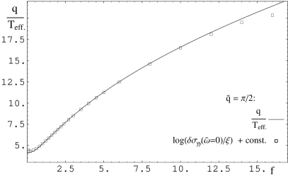
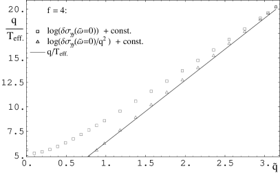
Figure 20: Left: $\log\,\delta\tilde{\sigma}_{yy}(\tilde{\omega}=0)/\xi$ (modulo a constant shift) and $\frac{\tilde{q}}{T_{eff}(f)}$ for $\tilde{q}=\pi/2$. The accuracy of the last two points are very sensitive to possible errors in $\delta\varepsilon_{0}$. Right: $\log\,\delta\tilde{\sigma}_{yy}(\tilde{\omega}=0)$ and $\frac{\tilde{q}}{T_{eff}(f)}$ for $f=4$. $\log\,\delta\tilde{\sigma}_{yy}(\tilde{\omega}=0)/\tilde{q}^{2}$ is shown to demonstrate the slow convergence due to polynomial factors of $\tilde{q}$.

For $\tilde{\omega}-\tilde{q}<0$, the finite-$\lambda$ correction becomes quickly negative and exponentially suppressed with increasing $f$ and $\tilde{q}$, roughly as described by the “effective temperature”, such that the exponential suppression does not get broken but is possibly modified. We show the shift $\frac{\delta\tilde{\sigma}_{yy}(\tilde{\omega}=0)}{\varepsilon_{0}\xi}$ as a function of $f$ for $\tilde{q}=0$ and a function of $\tilde{q}$ for $f=1$ in figure 20. Recall that figure 16 shows the same results for $\tilde{q}=0$.

The form of $\delta{\tilde{\sigma}}_{yy}$ for $f\lesssim 2$ is more similar to the resonances associated with the infinite-$\lambda$ result for ${\tilde{\sigma}}_{yy}$, as the amplitude seems to decay exponentially with ${\tilde{\nu}}$ and depends only polynomially on $\tilde{q}$, as we show in figure 18. Just as for the large $f$, the decay is slower than the one in the $0^{th}$ order term. This demonstrates that the effects of finite $\lambda$ are more significant for small $f$, where the length scales are still dominated by the $f=0$ length scale, that we can attribute to the strong coupling. Further it shows that the length scale due to the “width” of the defect has a tendency to persist.

6 Hall conductivity

The conductivity in section 3 is diagonal reflecting the parity invariance of the defect theory. Recently AdS/CFT techniques were applied to study Hall conductivity in the three-dimensional conformal field theories dual to an AdS₄ background [7, 8]. The construction in [7] involved breaking the parity invariance by introducing a background magnetic field. Of course, these calculations with a dyonic black hole could be easily emulated here by introducing additional background gauge fields on the AdS part of the probe branes — this would be a relatively straightforward extension of the analysis in, e.g., [49]. In [8], parity invariance is broken by the introduction of an auxiliary gauge field with a nonzero $\theta$-term. This construction is closely related to the following where we produce an off-diagonal conductivity by the addition of a topological $\theta$-term to the four-dimensional SYM action [50]. A related model of the quantum hall effect based on a probe brane construction appears in [16].

To introduce an $xy$ component to the conductivity, we begin by considering the Chern-Simons part of the D5-brane action. In particular, the latter includes the following term:

$$\Delta I=\frac{(2\pi\ell_{s}^{2})^{3}}{3!}N_{\textrm{\tiny f}}\,T_{5}\int C^{\textrm{\tiny[0]}}\,F\wedge F\wedge F$$ (6.91)

where $C^{\textrm{\tiny[0]}}$ is the RR scalar. Now the background (2.2) remains a consistent solution of the type IIB supergravity equations if we set this scalar to some arbitrary constant, i.e., $C^{\textrm{\tiny[0]}}=a$. Of course, this choice corresponds to adding a topological $\theta$-term to the action of the dual SYM theory [50]. Now if we recall the magnetic flux (2.6) on the internal $S^{2}$, the above contribution (6.91) reduces to the following four-dimensional action

$$\Delta I=(2\pi)^{4}\ell_{s}^{6}\,T_{5}\,2\pi\,a\,q\int F\wedge F\,,$$ (6.92)

where $q$ is the magnetic flux quantum number (2.6), indicating the number of D3-branes dissolved into the D5-brane. Thus upon integrating out the $S^{2}$ part of the probe brane geometry, this term (6.91) has become a topological $theta$-term for the four-dimensional worldvolume gauge fields. Since it is a topological term, it does not modify the equations of motion (3.44–3.47) for the gauge field. However, it does produce an additional boundary term,

$$\Delta I=2(2\pi)^{4}\ell_{s}^{6}\,T_{5}\,a\,q\int d^{3}\sigma\,\left[A_{y}\left(\partial_{t}A_{x}-\partial_{x}A_{t}\right)\right]_{u\to 0^{+}}\,,$$ (6.93)

which will modify the correlators. Note that we have simplified the above expression by assuming that in the cases of interest (as in previous sections) the gauge fields are independent of $y$. Introducing the Fourier transform (3.37), this boundary term becomes

$$\Delta I=-i4\pi\ell_{s}^{6}\,T_{5}\,a\,q\int d^{3}k\,\left[A_{y}(-k,u)\left(\omega\,A_{x}(k,u)+k_{x}\,A_{t}(k,u)\right)\right]_{u\to 0^{+}}\,.$$ (6.94)

Now following the same steps as in section 3.1, we arrive at the following off-diagonal contributions to the retarded Green’s function:

$$C_{xy}=i8\pi(2\pi\ell_{s}^{2})^{3}T_{5}\,a\,q\,\omega\,,\qquad C_{ty}=-i8\pi(2\pi\ell_{s}^{2})^{3}T_{5}\,a\,q\,k_{x}\,.$$ (6.95)

Note that in the $T=0$ limit, we expect this contribution to the Green’s function can be assembled in the Lorentz invariant expression:

$$\Delta C_{\mu\nu}=i\,\alpha\,\varepsilon_{\mu\nu\rho}\,k^{\rho}\,,$$ (6.96)

where $\alpha$ is the dimensionless constant:

$$\alpha=8\pi(2\pi\ell_{s}^{2})^{3}T_{5}\,a\,q=\frac{2\,a\,q}{\pi g_{\textrm{\tiny s}}}=\frac{8\,a\,q}{g_{\textrm{\tiny YM}}^{2}}\,.$$ (6.97)

The corresponding analysis in the D7 framework gives

$$\alpha_{\textrm{\tiny 7}}=16\pi^{2}(2\pi\ell_{s}^{2})^{4}T_{7}\,a\,q_{\textrm{\tiny 7}}=\frac{2a\,q_{\textrm{\tiny 7}}}{\pi g_{\textrm{\tiny s}}}=\frac{8\,a\,q_{\textrm{\tiny 7}}}{g_{\textrm{\tiny YM}}^{2}}\,.$$ (6.98)

While in principle, this form (6.96) need not be preserved at finite temperature, our results (6.95) calculated at finite $T$ indicates that in fact the form is preserved. Of course, this independence of the temperature is undoubtedly related to the topological nature of the $\theta$-term which is responsible for this off-diagonal contribution. It is amusing to note that since $q$ (and $q_{\textrm{\tiny 7}}$) is an integer, (6.97) and (6.98) take just the form of the integer quantum Hall effect, i.e., $\sigma_{xy}=\frac{n\,e^{2}}{2\pi}$ with $n\in\mathbb{Z}$. By this analogy, we would associate $e^{2}={4a}/{g_{\textrm{\tiny s}}}$.

7 Discussion

In this paper, we used holographic techniques to investigate the transport properties of certain defect CFT’s. In particular, we studied matter on a $(2+1)$-dimensional defect emersed in a heat bath of $(3+1)$-dimensional $N=4$ super-Yang-Mills plasma. Our analysis covers two distinct defect CFTs. The first was realized by embedding $N_{\textrm{\tiny f}}$ probe D5-branes in AdS${}_{5}\times S^{5}$, as described in section 2.1 and in this case, the system (at $T=0$) preserves eight supersymmetries. The second system involves embedding $N_{\textrm{\tiny f}}$ probe D7-branes in the AdS${}_{5}\times S^{5}$ background and the resulting defect CFT preserves no supersymmetries. In both cases, the theory could be deformed by introducing an additional internal flux on the probe branes. In the dual CFT, the defect then separated regions where the rank of the SYM gauge group was different. As described in section 2.2, this flux was crucial to remove an instability which would otherwise appear with the D7-brane construction. Perhaps surprisingly, the transport properties of both defect CFT’s were essentially identical.

Overall, our analysis revealed the expected diffusion-dominated hydrodynamic limit at small wave-numbers and we found a smooth crossover to a collisionless regime at the large wave-numbers. In the latter regime, the defect theory exhibits a conduction threshold, given by the wave-number $q$ of the current and the system is approximately described only in terms of the “rest-frame frequency” $\nu=\sqrt{\omega^{2}-q^{2}}$.

In many respects, our results coincided with those in [5], where holographic techniques were used to study a purely $(2+1)$-dimensional system with sixteen supersymmetries. Hence maximal supersymmetry (or supersymmetry, in general) does not seem to be a key feature for producing the interesting behaviour of these holographic models. Instead many properties seem to emerge from the infinite $N_{\textrm{\tiny c}}$ and infinite $\lambda$ limits, that are implicit in making a supergravity analysis of the AdS dual. In section 5, we elucidated one such effect that arises purely from the large-$N_{\textrm{\tiny c}}$ and large-$\lambda$ limits, namely the frequency independence of the conductivity, ${\tilde{\sigma}}(\tilde{\omega})$. In [5], this effect was described as a consequence of the electromagnetic duality of the gauge theory giving the dual description of the CFT currents. We were able to explicitly show that this duality is lost when stringy corrections are included in the worldvolume gauge field action and explicitly calculated the frequency dependence in ${\tilde{\sigma}}(\tilde{\omega})$ arising from the corresponding finite-$\lambda$ corrections to the conductivity. As described in appendix B, one can well imagine that there will be other interactions which, although they appear to be of higher order in the $\alpha^{\prime}$ expansion, provide further corrections to the conductivity $f^{n}/\sqrt{\lambda}$, where $n>2$. Hence, our results in section 5 are only the leading corrections when $f$ is small but finite. There will also be curvature interactions to the worldvolume action of the probe branes [47, 48]. These will also produce finite-$\lambda$ corrections but in contrast to the previous discussion, the latter will not be enhanced by factors of $f$ and first appear only at order $1/\lambda$. While a completely consistent set of curvature terms is not known at this time, the effect of certain representative terms was considered in [24].

While certain aspects of charge transport were similar for the present defect CFT’s and the maximally supersymmetric CFT studied in [5], we also found some profound differences. The most prominent is the dependence of our results on the internal flux $f$, certainly a difference since no such parameter exists in the maximally supersymmetric case. For example then, with a large $f$, strong quasiparticle peaks appeared in the spectral functions and conductivities. Similarly, certain phenomena in the defect CFT seemed to be controlled by a new dynamically generated scale in this regime, i.e., a scale distinct from the temperature $T$. We denoted this scale as the effective temperature $T_{eff}$ in section 3.2.1. For small $f$, $T_{eff}\sim T$ to within factors of order one. However, for large $f$, one finds that $\pi T/(2T_{eff})\simeq k\,\sqrt{f}$ where $k=4\Gamma(5/4)^{2}/\sqrt{\pi}$, as shown in (3.2.1). While this seems a curious way to present the ratio of $T$ and $T_{eff}$, it was found in section 4.2 that precisely this combination played a role in fixing the spacing of the quasiparticle poles. Further, as also noted there, precisely the same behaviour was found at large $f$ for the diffusion constant: $\pi\,D\,T\simeq k\,\sqrt{f}$.

A more intuitive picture as to the origin of this dynamical scale comes from considering the probe brane geometry, as in section 2. Recall that when $f$ is nonvanishing, the defect separates a region where the SYM has gauge group $U(N_{\textrm{\tiny c}}+q)$ from one where the gauge group is $U(N_{\textrm{\tiny c}})$. However, on the side where the rank of the gauge group is enhanced, the defect also excites a noncommutative configuration of adjoint scalars in a $U(q)$ subgroup of the full $U(N_{\textrm{\tiny c}}+q)$. At $T=0$, this configuration extends to infinity with ${\rm Tr}(\Phi^{2})={q^{2}\over 4N_{\textrm{\tiny f}}}\,{1\over z^{2}}$. In particular, this configuration preserves the conformal symmetry, i.e., does not introduce a new scale. The scalar profile is reflected in the radial profile of the probe D-branes which also extends out to $z\rightarrow\infty$ when $T=0$ and $f$ is nonvanishing. However, when the temperature is nonvanishing, the probe branes fall into the horizon at a finite value of $z$. For large $f$, one finds

$$z_{max}\,T=k\,\sqrt{f}\,,$$ (7.99)

where $k$ is precisely the same constant found above. The natural interpretation of this profile is that at finite temperature, thermal fluctuations decohere the scalar fields at some distance away from the defect. That is, at finite $T$, the defect can only excite a coherent configuration of scalars out to $z_{max}$. However, at small $f$, $z_{max}$ vanishes whilst the dynamical length scale doesn’t vanish. We can interpret that by some extra contribution to the width that arises from excitations in the bulk fields that are induced at strong coupling from the presence of the charged matter degrees of freedom on the defect.

One interpretation then is that the defect effectively acquires a finite width when $T$ is nonvanishing. This intuitive picture may seem more reasonable, if we recall that the system is at (extremely) strong coupling and so any probe exciting of the defect fields will actually excite a complicated mixture of defect fields and “bulk” SYM fields. This picture of finite-width for the defect seems to match well with the results for the quasiparticle spectrum on the defect. In particular, we found that both the conduction threshold and the resonance peaks are well-described by a quasiparticle “tower” with equally spaced “rest frame” energy and constant “mass to inverse lifetime ratio”. The length scale that is suggested from this spectrum is very similar to $\pi DT$ and $\pi T/(2T_{eff})$ (and at large $f$ also similar to $z_{max}$) plus a small constant.

In terms of the effective Schrödinger analysis, e.g., see appendix C, the quasinormal spectrum arises in the gravity side from interference on a potential barrier in the asymptotic region. From the profile of the brane, this translates into an interference or resonance in the region around the defect. These two dual pictures of the origin of the spectrum seem orthogonal. The intuitive CFT picture involves a width and implicitly, a potential, in the space transverse to the defect, while the effective Schrödinger analysis constructs an effective potential in the radial or “energy scale” direction. It would certainly be interesting to have a clearer connection between these two descriptions.

The hydrodynamic and collisionless regimes are cleanly separated at a critical wave-number where the diffusion pole disappears, as observed in section 4.3. There, we found that the diffusion mode is partnered with another dissipative mode on the imaginary axis. These two poles coalesce at the critical wave-number and move out into the complex plane for larger $q$. Hence precisely at the critical wave-number $q_{c}$, the corresponding thermal correlator will exhibit a curious double pole on the imaginary axis. Interestingly, $q_{c}$ has a similar qualitative $f$ dependence as the other (inverse) length scales and is also quantitatively close, as $q_{c}/(\pi T)\sim 0.67/(k\sqrt{f})$. This supports again the concept that the properties of the defect are controlled by one fundamental length scale, that can be related to the effective width of the defect.

In section 6, we outlined a topological Hall conductivity, which is induced when the defect is coupled to the SYM gauge theory with a topological $\theta$-term. Of course, it would also be interesting to study the Hall conductivity induced by a background magnetic field on the defect. Other interesting directions would be to study the effect of a finite mass for the defect fields or of a finite chemical potential. With these additional parameters, there are many non-trivial physical properties of the defect related to condensed matter physics that one can study through the transport properties. We will address these questions in an upcoming paper [51].

Appendix A Diffusion constant on the defect

The worldvolume gauge field corresponds to a conserved current on the defect in the dual CFT. In the hydrodynamic regime, one then expects to see the diffusion of the conserved charge according to Fick’s law:

$$\partial_{t}\,j^{0}=D\ \vec{\nabla}^{2}j^{0}\,.$$ (A.100)

This expectation can be confirmed in a holographic context [52, 53, 54] and, in fact, the computation of the diffusion constant $D$ can be performed in a number of different ways. In the following, we use the membrane paradigm approach.

The computation of the diffusion constant via the membrane paradigm was discussed in [52] where explicit formulae for various transport coefficients in terms of metric components for a wide class of backgrounds were derived. There, the authors considered perturbations of a black brane background and a formula for the diffusion constant (eq. (2.27) in [52]) resulted from a derivation of Fick’s law. An analogous computation can be performed for the D5-branes’ vector field for black hole embeddings considered here, with the result

$$D = \left.\frac{\sqrt{-g}}{\sqrt{h}}\frac{1}{g_{xx}\sqrt{-g_{tt}g_{\rho\rho}}}\right|_{\rho=1}\ \int d\rho\left(-g_{tt}\,g_{\rho\rho}\,\frac{\sqrt{g_{\rm int}}}{\sqrt{-g}}\right)$$ (A.101)

$$= \frac{(1+f^{2})^{1/2}}{\pi T}\int_{0}^{1}\frac{du}{\sqrt{1+f^{2}u^{4}}}\equiv\frac{(1+f^{2})^{1/2}}{\pi T}\,I(f)\,.$$

In the first expression above, the metric $g$ is the induced metric on the D5-branes (2.7) and $g_{\rm int}$ is the determinant of the metric on the internal two-sphere (with unit radius). The integral can be evaluated analytically yielding a hypergeometric function:

$$I(f)\,=\,{}_{2}F_{1}(\frac{1}{4},\frac{1}{2};\frac{5}{4};-f^{2})$$ (A.102)

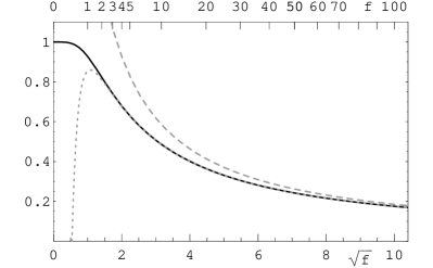
Figure 21: The integral $I(f)$ plotted as a function of $\sqrt{f}$: The solid line is the exact result as given in eq. (A.102). The upper dashed (lower dotted) line corresponds to the first term (first two terms) in the large $f$ expansion in eq. (A.108).

Figure 21 shows a plot of $I(f)$.

This same integral in eq. (A.101) reappears at various points in our analysis and so it is useful to gain some better intuition for this expression. First, let us rewrite the integral as

$$I(f)\,=\,f^{-1/2}\int_{0}^{f^{1/2}}\frac{ds}{\sqrt{1+s^{4}}}\ .$$ (A.103)

Now, we find that we can expand the integrand around $s=0$ as

$$\frac{1}{\sqrt{1+s^{4}}}\,\sim\,1\,-\,\frac{1}{2}s^{4}\,+\,\frac{3}{8}s^{8}\,+\,\ldots\,$$ (A.104)

and around $s=\infty$

$$\frac{1}{\sqrt{1+s^{4}}}\,\sim\,\frac{1}{s^{2}}\big{(}1\,-\,\frac{1}{2}s^{-4}\,+\,\frac{3}{8}s^{-8}\,+\ldots\big{)}\,.$$ (A.105)

At $s=1$, the convergence of both sequences goes as $\frac{1}{n!}$ and a more precise approximation is

$$\frac{1}{\sqrt{1+s^{4}}}\,\sim\,\frac{1}{\sqrt{2}}(1-(s-1)+\ldots)\ .$$ (A.106)

Combining (A.103) with these expansions, we can find the integral in various approximations

$$f\ll 1\,:~{}~{}~{}~{}I(f) \sim 1\,-\,\frac{1}{10}f^{2}\,+\,\frac{3}{72}f^{4}\,+\ldots$$ (A.107)

$$f\gg 1\,:~{}~{}~{}~{}I(f) \sim c_{\infty}f^{-1/2}\,-\,f^{-1}\,+\,\frac{1}{10}f^{-3}-\,\frac{3}{72}f^{-5}\,+\ldots$$ (A.108)

$$f\sim 1\,:~{}~{}~{}~{}I(f) \sim f^{-1/2}\Big{(}c_{1}\,+\,\frac{1}{\sqrt{2}}\big{(}(f^{1/2}-1)\,-\,\frac{1}{2}(f^{1/2}-1)^{2}\,+\ldots\big{)}\Big{)}$$ (A.109)

where $c_{1}=\int_{0}^{1}\frac{ds}{\sqrt{1+s^{4}}}=2\pi^{-1/2}\Gamma^{2}\big{(}\frac{5}{4}\big{)}$ and $c_{\infty}=\int_{0}^{\infty}\frac{ds}{\sqrt{1+s^{4}}}=2c_{1}\simeq 1.854$. Further, we note that the expansion about $s=0$ is just the expansion of the hypergeometric function as a hypergeometric series.

Hence, at small and very large $f$, we have for the diffusion constant

$$D\,T\rightarrow\left\{\begin{matrix}\frac{1}{\pi}&\qquad{\rm with}\ f\rightarrow 0\,,\cr\frac{c_{\infty}}{\pi}\sqrt{f}&\qquad{\rm with}\ f\rightarrow\infty\,.\cr\end{matrix}\right.$$ (A.110)

We note that the $f=0$ result is different from but close to the value found for M2-brane hydrodynamics [55]: $D\,T=3/4\pi$. Also note that in the limit of large $f$, the diffusion constant grows as $\sqrt{f}$.

Appendix B Corrections to D5-brane action

The worldvolume action (2.4) is a low-energy effective action which captures the interactions of the massless open string modes supported on the D5-branes. The “stringy” nature of the underlying theory will in principle produce an infinite series of higher dimension terms that are suppressed at low energies by the inverse string tension, i.e., $\alpha^{\prime}\equiv\ell_{\textrm{\tiny s}}^{2}$. However, in practice, one typically only includes a specific set of terms to a certain order in the $\alpha^{\prime}$ expansion. In fact, the action (2.4) implicitly captures an infinite set of these stringy corrections, as can be seen by the explicit factor of $\ell_{\textrm{\tiny s}}^{2}$ accompanying the gauge field strength in the DBI action. Further, we might add that this entire series of terms plays a role in our analysis, as the full square-root form of the action is used in (2.8) to normalize the DBI contributions. However, as already alluded to in section 2.2, the DBI action does not capture all of the higher dimension stringy interactions. Beyond the nonabelian commutator terms referred to there, the full low-energy action includes additional terms involving derivatives of the gauge field strength [45, 46], as well as higher derivative couplings to the bulk fields [47, 48]. In terms of the dual CFT, the contributions of these $\alpha^{\prime}$ interactions will provide finite $\lambda$ corrections to the leading supergravity results.

In the following and in section 5, we focus our attention on a particular new term involving derivatives of the field strength, which modifies the vector correlators on the D5-branes. Our results below give the leading $1/\lambda$ corrections when $f$ is finite. Our calculations consider explicitly those leading contributions for the transverse correlator. As we discuss in section 5, the higher derivative interaction also upsets the electromagnetic duality on the AdS₄ part of the worldvolume.

An effective action to describe open string gauge fields at higher order in $\alpha^{\prime}$ has been extensively studied in the literature, e.g., see [45, 46]. However, since we consider only the linearized equations of motion (or the quadratic action) to compute the correlators in the $AdS_{4}$ directions, the leading term at $\mathscr{o}(\alpha^{\prime 3})$ is [45]

$$-\frac{1}{4g_{4}^{2}}\,\frac{\zeta(3)}{16\pi^{4}}\,\frac{(2\pi\ell_{s}^{2})^{3}}{L^{2}\sqrt{1+f^{2}}}\int d^{6}\sigma\sqrt{-g}\,\nabla_{\mu}F_{\alpha\beta}\nabla^{\mu}F^{\alpha\beta}\,F^{2}\ .$$ (B.111)

In fact, this term only becomes relevant for the calculation of the vector correlators because of the flux background on the compact $S^{2}$. After integrating over the internal two-sphere, this interaction reduces to

$$-\frac{1}{4g_{4}^{2}}\,\frac{\zeta(3)}{2\pi}\,\frac{\ell_{s}^{2}\,f^{2}}{\sqrt{1+f^{2}}}\int d^{4}\sigma\sqrt{-g}\,\nabla_{\mu}F_{\alpha\beta}\nabla^{\mu}F^{\alpha\beta}\ .$$ (B.112)

Note that the background flux (2.6) remains unmodified by this new interaction. When considering linearized fluctuations of the vector field, we can work with a perturbative expansion in $\ell_{\textrm{\tiny s}}^{2}/L^{2}=1/\sqrt{\lambda}$. We begin with the Ansatz

$$F=F^{\!(0)}+\frac{\ell_{\textrm{\tiny s}}^{2}}{L^{2}}\,F^{\!(1)}+\cdots\ .$$ (B.113)

The equations determining the leading $0^{th}$ order field are still the same Maxwell equations (3.34), while for $F^{\!(1)}$, we have

$$\nabla_{\nu}F^{\!(1)\,\nu\mu}\,=\,\frac{\zeta(3)}{2\pi}\frac{L^{2}\,f^{2}}{\sqrt{1+f^{2}}}\nabla_{\nu}\nabla_{\alpha}\nabla^{\alpha}F^{\!(0)\,\nu\mu}\,.$$ (B.114)

Writing this out explicitly for $\mu=y$ gives

$$\partial_{u}\frac{h}{\sqrt{H}}\partial_{u}A^{\!(1)}_{y}+\frac{\sqrt{H}}{h}(\tilde{\omega}^{2}-h\tilde{q}^{2})\partial_{u}A^{\!(1)}_{y}$$ (B.115)

$$\qquad=\,\frac{\zeta(3)f^{2}}{2\pi\sqrt{1+f^{2}}}\left(\partial_{u}\,u^{2}\sqrt{\frac{h}{H}}\partial_{u}\,\frac{h}{u^{2}\sqrt{H}}\partial_{u}\,u^{2}\sqrt{\frac{h}{H}}\partial_{u}A^{\!(0)}_{y}\,+\,\partial_{u}\,\frac{u^{2}}{\sqrt{H}}(\tilde{\omega}^{2}-\tilde{q}^{2}h)\partial_{u}A^{\!(0)}_{y}\,\right.$$

$$\qquad\ \ +\,\left.\frac{\tilde{\omega}^{2}u^{2}}{\sqrt{h}}\partial_{u}\,\frac{h}{u^{2}\sqrt{H}}\partial_{u}\,\frac{u^{2}}{\sqrt{h}}A_{y}-\tilde{q}^{2}u^{2}\partial_{u}\,\frac{h}{u^{2}\sqrt{H}}\partial_{u}\,u^{2}A^{\!(0)}_{y}+\frac{u^{2}\sqrt{H}}{h^{2}}\left(\tilde{\omega}^{2}-\tilde{q}^{2}h\right)^{2}A^{\!(0)}_{y}\right)\,.$$

Note that we adopt the convention above that the derivatives $\partial_{u}$ act on all factors to their right. At the horizon, $u\to 1$, we again wish to impose infalling boundary conditions. If we substitute the expansion (3.52) for $A_{y}$ as $u\to 1$, the right hand side of (B.115) diverges as $h^{i\tilde{\omega}/4-2}$ and hence we expect to find singular behaviour in $A^{\!(1)}_{y}$ there. Hence we begin by isolating this singular behaviour in a particular solution to (B.115): $A^{\!(1),NHG}_{y}\sim h^{i\tilde{\omega}/4}(\frac{a}{h}+b+c\log h\,+d\,h\,\log h)$ with appropriate constants $a,b,c,d$. This particular solution is holds to order $h^{0}$ near $u\to 1$ and is well-behaved in the rest of the geometry. Implicitly, it also satisfies the desired infalling boundary conditions. Next we add to $A^{\!(1),NHG}_{y}$ a contribution which is regular at the horizon and takes the form on an infalling homogenous solution near $u\to 1$ as described by (3.52) and (3.53). That is, we use the Ansatz

$$A^{\!(1)}_{y}\,=\,A^{\!(1),NHG}_{y}+h^{i\tilde{\omega}/4}\left(1+\left(\frac{i\tilde{\omega}}{4}\frac{3+5f^{2}}{1+f^{2}}+\frac{\tilde{q}^{2}}{4+2i\tilde{\omega}}\right)(1-u)\right)\mathscr{F}(u)\ .$$ (B.116)

where $\partial_{u}\mathscr{F}(u)|_{u\to 1}=0$. This Ansatz is constructed so that $\mathscr{F}(u)$ is well behaved everywhere and we proceed by calculating this profile numerically. In practise, we apply the boundary condition at some small, but finite, $(1-u)$, so need we go one order higher in $h$ and increase the accuracy for solving $A^{\!(0)}$.

The correlator is then found by substituting our original Ansatz (B.113) into (3.41),

$$C_{yy}\,=\,\frac{\varepsilon_{0}}{\sqrt{1+f^{2}}}\frac{\partial_{u}(A^{\!(0)}_{y}+\ell_{\textrm{\tiny s}}^{2}/L^{2}\,A^{\!(1)}_{y})}{A^{\!(0)}_{y}+\ell_{\textrm{\tiny s}}^{2}/L^{2}\,A^{\!(1)}_{y}}\,\simeq\,\frac{\varepsilon_{0}}{\sqrt{1+f^{2}}}\left[\frac{\partial_{u}A^{\!(0)}_{y}}{A^{\!(0)}_{y}}+\frac{\ell_{\textrm{\tiny s}}^{2}}{L^{2}}\,\partial_{u}\left(\frac{A^{\!(1)}_{y}}{A^{\!(0)}_{y}}\right)\right]_{u\to 0}+\cdots\,.$$ (B.117)

From this expression, we can see that the normalization of any homogenous solution in $A^{\!(1)}_{y}$ does not effect the correlator, as we expect for a gauge-invariant quantity. The expressions for $C_{tt}$ and $C_{xx}$ following from (3.42) are similar to that above.

The second term on the right-hand side of (B.117) yields the correction to the correlator due to the fact that the solutions for the fluctuations $A_{\mu}(u)$ are modified. In addition, (B.112) also contributes to the overall value of the bulk action and hence provides an additional modification of the correlators. Proceeding as in (3.36), we now get two boundary terms at order $\ell_{\textrm{\tiny s}}^{2}$, since $D_{\mu}F_{\alpha\beta}D^{\mu}F^{\alpha\beta}=D_{\mu}(F_{\alpha\beta}D^{\mu}F^{\alpha\beta})-D_{\alpha}(A_{\beta}D_{\mu}D^{\mu}F^{\alpha\beta})+A_{\beta}(e.o.m.)^{\beta}$, where the last term combines with contributions from the leading Maxwell term in the action to vanish by the equations of motion. These expressions lead to a number of new contributions to the flux (3.40), which in principle even contribute to off-diagonal correlators. We might add that there is a further ambiguity in these expressions because the effective action (B.112) was constructed from examining string scattering amplitudes [45] and so it is only determined up to total derivatives or boundary terms. Explicitly comparing [45] and [46], one finds that in fact their results differ by such a boundary term. However, this ambiguity does not contribute in our background (3.35) and in fact, of the myriad of potential boundary contributions, only a single term survives

$$\Delta C_{yy}\,=\,-\frac{\ell_{\textrm{\tiny s}}^{2}\,f^{2}\zeta(3)}{2\pi\sqrt{1+f^{2}}}\,\frac{\varepsilon_{0}}{\sqrt{1+f^{2}}}\left.\frac{\nabla^{2}\partial_{u}A_{y}}{A_{y}}\right|_{u\to 0}\ .$$ (B.118)

Similar expressions survive for $C_{tt}$ and $C_{xx}$ while the potential contributions to the off-diagonal correlators vanish. Combining the results in (B.117) and (B.118), we can write the total change to the correlator as

$$\delta C_{yy}\,=\,\frac{\ell_{\textrm{\tiny s}}^{2}}{L^{2}}\,\frac{\varepsilon_{0}}{\sqrt{1+f^{2}}}\,\left[\partial_{u}\left(\frac{A^{\!(1)}_{y}}{A^{\!(0)}_{y}}\right)-\frac{L^{2}f^{2}\zeta(3)}{2\pi\sqrt{1+f^{2}}}\frac{\nabla^{2}\partial_{u}A^{\!(0)}_{y}}{A^{\!(0)}_{y}}\right]_{u\to 0}\ .$$ (B.119)

Again similar expressions arise for $\delta C_{tt}$ and $\delta C_{xx}$.

The two previous formulae, (B.118) and (B.119), still require a precise definition for $\nabla^{2}\partial_{u}A_{y}$. This expression should understood as the covariant tensor expression $\nabla^{2}F_{uy}$ which when evaluated asymptotically yields a remarkably simple result:

$$\nabla^{2}\partial_{u}A_{y}=-\frac{2}{L^{2}}\,\frac{1}{1+f^{2}}\,\partial_{u}A_{y}+\cdots$$ (B.120)

where the implicit terms decay rapidly enough as $u\to 0$ that they will not contribute to the correlator. Hence (B.118) can be greatly simplified to

$$\Delta C_{yy}\,=\,\frac{\ell_{\textrm{\tiny s}}^{2}}{L^{2}}\frac{f^{2}\zeta(3)}{\pi(1+f^{2})^{3/2}}\frac{\varepsilon_{0}}{\sqrt{1+f^{2}}}\left.\frac{\partial_{u}A_{y}}{A_{y}}\right|_{u\to 0}\ .$$ (B.121)

The last factor has exactly the same form as the leading correlator (3.41) and so this contribution can be interpreted in terms of a rescaling of the pre-factor $\varepsilon_{0}$:

$$\varepsilon_{0}\to\varepsilon_{0}\left(1+\frac{1}{\sqrt{\lambda}}\frac{f^{2}\,\zeta(3)}{\pi(1+f^{2})^{3/2}}\right)\ ,$$ (B.122)

where we have replaced $\ell_{\textrm{\tiny s}}^{2}/L^{2}=1/\sqrt{\lambda}$. Remarkably our numerical calculations show that the first contribution to $\delta C_{yy}$ in (B.119) also produces a shift of $\varepsilon_{0}$ with precisely the same $f$ dependence – see figure 14.

At this point, several comments are in order. We already pointed out that the square-root form of the DBI action already incorporates an infinite set of stringy $\alpha^{\prime}$ corrections. While this form was incorporated in our leading order calculations, e.g., (2.8), it did not appear to introduce any $1/\lambda$ corrections. Of course, these factors are hidden in the definition (2.9) of $f$ and for finite values of $f$, we are actually introducing a magnetic flux quantum number $q\sim O(\sqrt{\lambda})$. In this context, it is not quite correct to say the interaction (B.111) is the leading term to modify the correlators. One can well imagine that there will be other interactions which, although they appear to be of higher order in the $\alpha^{\prime}$ expansion, will modify the correlator with contributions of order $f^{n}/\sqrt{\lambda}$ where $n>2$. Of course, these contributions will be suppressed in a regime where $f\ll 1$. Considering the possible tensor structure of the relevant higher order interactions, it seems that this class of contributions will always be arising from an equation of motion of the form (B.114).

Appendix C Hyperbolic tangent potential

To get more insight into the appearance of the finite temperature effects in the frequency dependence of the conductivity, we can study a qualitatively similar problem that has an analytic solution.

C.1 Finding the spectral curves

Let us modify the effective Schrödinger equation in (3.79) to write it in terms of the complex frequency $\nu$ of section 4, i.e., $\tilde{\nu}\equiv\sqrt{\tilde{\omega}^{2}-\tilde{q}^{2}}$,

$$\qquad\qquad\ \ \ \ \ \left(-\partial_{\rho}^{\,2}+V\right)A_{y}\,=\,\tilde{\nu}^{2}A_{y}$$ (C.123)

$${\rm with}\qquad V=-\tilde{q}^{2}\,u^{4}\quad{\rm and}\quad\rho\,=\,\int_{0}^{u}d\tilde{u}\frac{\sqrt{H}}{h}\ .$$

Recall in terms of the new radial coordinate $\rho$, the asymptotic boundary is mapped to $\rho=0$ and the horizon, to $\rho\to\infty$. In fact, it is straightforward to evaluate the integral above to find $\rho(u)$ in terms of incomplete elliptic integrals of the third kind or alternatively, in terms of the Appell hypergeometric function [56] $\rho=\sqrt{1+f^{2}}u\,F_{1}\left(\frac{1}{4};\frac{1}{2},1;\frac{5}{4};-f^{2}u^{4},u^{4}\right)$. Note that the only difference between (3.79) and (C.123) is that we have subtracted $\tilde{q}^{2}\,A_{y}$ from both sides in the equation above. Hence in the present form, the effective potential $V$ vanishes at $\rho=0$ and approaches $-\tilde{q}^{2}$ as $\rho\to\infty$.

The equation of motion in the form of (C.123) can be examined in three distinct regions which for $f\gg 1$, where the potential looks roughly like

$$V\ \sim\ 0 : \rho\lesssim f^{1/2}$$

$$V\ \sim\ -\tilde{q}^{2}(2f^{1/2}-\rho)^{-4} : f^{1/2}\lesssim\rho\lesssim 2f^{1/2}-1$$

$$V\ \sim\ -\tilde{q}^{2}+\tilde{q}^{2}e^{-4(\rho-2f^{1/2}+1)} : 2f^{1/2}-1\lesssim\rho\ .$$ (C.124)

Of course, the full potential is smooth across these three regions.

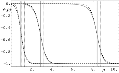
Figure 22: The exact potential $V$ (solid grey) and the $\tanh$ approximation $V_{app}$ (black dotted), for $f\in\{0,4,25\}$ with $\tilde{q}=1$. We also indicate a number of interesting values of $\rho$ with narrow vertical lines: $\rho(u_{half})$, solid black; $\rho(u_{min})$, solid grey; $\rho=\frac{\pi\,T}{2\,T_{eff}}$, dashed black; and $\rho=\pi\,D\,T$, grey dashed.

To model the “smooth” step with a finite slope and a fast tailoff in the asymptotic regions, we will use

$$V_{app}\,=\,-\tilde{q}^{2}\frac{1\,+\,\tanh\,\mathfrak{n}(\rho-\rho_{0})}{2}\ ,$$ (C.125)

which allows us to find exact solution for (C.123). We fix the “step” position $\rho_{0}$ either as location where the the potential has half its minimum, i.e., at $u_{half}^{4}=1/2$ or the point where the slope of the potential is minimum, i.e., at

$$u_{min}^{4}=\frac{5f^{2}-7+\sqrt{(7-5f^{2})^{2}+108f^{2}}}{18f^{2}}\ .$$ (C.126)

To fix the parameter $\mathfrak{n}$ that we will use to characterize the slope of the step of the potential, we simply take the slope of the full potential at either of the corresponding points: $\mathfrak{n}\equiv-2\left.\partial_{\rho}V\right|_{u_{half,min}}=8\tilde{q}^{2}u^{3}h(u)H(u)^{-1/2}\big{|}_{u_{half,min}}$. Working with $u_{half}$ or $u_{min}$ will give $V_{app}$ which is a good approximation of the full potential $V$. As shown in figure 22, the potentials constructed with these two choices typically can not be distinguished. For comparison purposes, the figure also indicates two other interesting scales: $\rho={\pi\,T}/{2T_{eff}}$ and $\pi\,D\,T$. There we see that both of these scales are close to the width of the effective potential but $\rho=\pi\,D\,T$ is particularly close to the center of the step.

Note that $V(\rho=0)=0$ and $\partial_{\rho}V(\rho=0)=0$ while neither of these properties holds for the approximation (C.125). We will take account of this fact simply by expanding around $\rho-\rho_{0}\rightarrow-\infty$ and discarding higher order terms when computing the values at $\rho=0$. One can expect this potential to be a good approximation for ${\tilde{\nu}}\gg 1$, where the result is less sensitive to the details of the potential away from it’s maximum slope and for large $f$, where the results should be dominated by the large flat part of the potential.

Using infalling boundary conditions at $\rho\rightarrow\infty$, the solution is

$$A_{y} = A_{y0}\,{}_{2\!}F_{1}{\scriptstyle\left(1+\frac{i{\tilde{\nu}}}{2\mathfrak{n}}(1-\sqrt{1+\tilde{q}^{2}/{\tilde{\nu}}^{2}}),\,\frac{i{\tilde{\nu}}}{2\mathfrak{n}}(1-\sqrt{1+\tilde{q}^{2}/{\tilde{\nu}}^{2}});\,1-\frac{i{\tilde{\nu}}}{\mathfrak{n}}\sqrt{1+\tilde{q}^{2}/{\tilde{\nu}}^{2}};\,\frac{1}{1+e^{2\mathfrak{n}(\rho-\rho_{0})}}\right)}$$ (C.127)

$$\ \ \ \ \ \ (1-\tanh\,\mathfrak{n}(\rho-\rho_{0}))^{-\frac{i{\tilde{\nu}}}{2\mathfrak{n}}\sqrt{1+\tilde{q}^{2}/{\tilde{\nu}}^{2}}}(1+\tanh\,\mathfrak{n}(\rho-\rho_{0}))^{\frac{i{\tilde{\nu}}}{2\mathfrak{n}}}$$

and the asymptotic expansion gives us

$$A_{y} = A_{y0}\,e^{i{\tilde{\nu}}(\rho-\rho_{0})}\left(\frac{\left(\sqrt{1+\tilde{q}^{2}/{\tilde{\nu}}^{2}}-1\right)\,\,\Gamma\!\left(\frac{i{\tilde{\nu}}}{2\mathfrak{n}}(1-\sqrt{1+\tilde{q}^{2}/{\tilde{\nu}}^{2}})\right)^{2}\,\,\Gamma\!\left(-\frac{i{\tilde{\nu}}}{\mathfrak{n}}\right)}{\left(\sqrt{1+\tilde{q}^{2}/{\tilde{\nu}}^{2}}+1\right)\,\Gamma\!\left(-\frac{i{\tilde{\nu}}}{2\mathfrak{n}}(\sqrt{1+\tilde{q}^{2}/{\tilde{\nu}}^{2}}+1)\right)^{2}\,\Gamma\!\left(\frac{i{\tilde{\nu}}}{\mathfrak{n}}\right)}\,+\,e^{-2i{\tilde{\nu}}(\rho-\rho_{0})}\right)$$ (C.128)

$$\equiv A_{y0}\,e^{i{\tilde{\nu}}(\rho-\rho_{0})}\left(\aleph\,+\,e^{-2i{\tilde{\nu}}(\rho-\rho_{0})}\right)\ ,$$

for which we redefined $A_{y0}$. In the opposite limit, as $\rho\rightarrow\infty$, the solution converges exponentially to $A_{y}\propto e^{-i{\tilde{\nu}}\rho\sqrt{1+\tilde{q}^{2}/{\tilde{\nu}}^{2}}}$, which is the desired infalling wave solution at the horizon.

The transverse conductivity can now be written in a compact suggestive form in terms of the implicitly defined $\aleph$:

$$\tilde{\sigma}_{yy}\,=\,\varepsilon_{0}\,{\mbox{Re }}\frac{{\tilde{\nu}}}{\tilde{\omega}}\frac{\aleph\,-\,e^{2i{\tilde{\nu}}\rho_{0}}}{\aleph\,+\,e^{2i{\tilde{\nu}}\rho_{0}}}\,,$$ (C.129)

which is of the same form as the result (3.2.2), but with different coefficients. We again see how the oscillatory pattern arises from interference in the asymptotic region due to the potential “step”, and how the effective temperature arises from tunnelling through the potential out of the “heat bath” in the near horizon region. For $|{\tilde{\nu}}|\gg\mathfrak{n}$, we find the limit

$$\aleph\,\stackrel{{\scriptstyle|{\tilde{\nu}}|\rightarrow\infty}}{{\longrightarrow}}\,\frac{4\mathfrak{n}{\tilde{\nu}}}{\mathrm{sgn}({\mbox{Re }}{\tilde{\nu}})\,\pi\tilde{q}^{2}}e^{\mathrm{sgn}({\mbox{Re }}{\tilde{\nu}})\,\pi{\tilde{\nu}}/\mathfrak{n}}\left(1+\mathscr{O}\left({\scriptstyle\frac{\tilde{q}}{{\tilde{\nu}}}}\,\log\,{\tilde{\nu}}/\mathfrak{n}\right)\right)\ ,$$ (C.130)

This result shows that the subleading term in the conductivity (beyond the low temperature limit (3.51)) has an exponential frequency dependence for $\tilde{\omega}>\tilde{q}$, as we found in section 3.2.1. We can also see how the results depend on $\mathfrak{n}$, i.e., on the slope of the step in the potential. We compare the present results (C.129) for the conductivity to our numerical results and to the perturbative approximation in figure 8. There we can see that the various approaches are in very close agreement for $\tilde{\omega}\gtrsim\tilde{q}$.

C.2 Exact pole structure

We can look at the solutions (C.128) and identify the quasinormal modes by imposing the asymptotic boundary condition: $A_{y}(\rho=0)=0$. The quasinormal frequencies are then simply determined by the equation

$$e^{2i{\tilde{\nu}}\rho_{0}}\,=\,-\frac{\left(\sqrt{1+\tilde{q}^{2}/{\tilde{\nu}}^{2}}-1\right)\,\Gamma\!\left(\frac{i{\tilde{\nu}}}{2\mathfrak{n}}(1-\sqrt{1+\tilde{q}^{2}/{\tilde{\nu}}^{2}})\right)^{2}\,\Gamma\!\left(-\frac{i{\tilde{\nu}}}{\mathfrak{n}}\right)}{\left(\sqrt{1+\tilde{q}^{2}/{\tilde{\nu}}^{2}}-1\right)\,\Gamma\!\left(-\frac{i{\tilde{\nu}}}{2\mathfrak{n}}(1+\sqrt{1+\tilde{q}^{2}/{\tilde{\nu}}^{2}})\right)^{2}\,\Gamma\!\left(\frac{i{\tilde{\nu}}}{\mathfrak{n}}\right)}$$ (C.131)

which simplifies in the limit of $|{\tilde{\nu}}|\gg\mathfrak{n},\tilde{q}$ to

$$e^{(2i\rho_{0}-\mathrm{sgn}({\mbox{Re }}{\tilde{\nu}})\,\pi/\mathfrak{n}){\tilde{\nu}}}\,\simeq\,-\frac{4\mathfrak{n}{\tilde{\nu}}}{\mathrm{sgn}({\mbox{Re }}{\tilde{\nu}})\,\pi\tilde{q}^{2}}\ .$$ (C.132)

These quasinormal frequencies also give the location of the poles in the spectral function [36, 57], with the exception of the asymptotically constant solution, ${\tilde{\nu}}=0$. In the terminology of section 4, the present approximation yields:

$${\tilde{\nu}}_{0}=\frac{4\pi\rho_{0}}{4\rho_{0}^{2}+\pi^{2}/\mathfrak{n}^{2}}\ ,\qquad\frac{{\tilde{\gamma}}_{0}}{{\tilde{\nu}}_{0}}=\frac{\pi}{2\rho_{0}\mathfrak{n}}\ .$$ (C.133)

Further as mentioned in section 4, the subleading contributions are logarithmic in $n$, giving us

$$\delta{\tilde{\nu}}_{n}=\frac{{\tilde{\gamma}}_{0}-i{\tilde{\nu}}_{0}}{2\pi}\big{(}\ln n+\ln\frac{4\mathfrak{n}(i\gamma_{0}-{\tilde{\nu}}_{0})}{\pi\tilde{q}^{2}}\big{)}\ ,$$ (C.134)

in contrast to the constant shift as the largest subleading term for the full correlator.

The residues in the Green’s function, before taking the imaginary part, are given by

$$\mathscr{R}_{yy}^{(n)}\,\equiv\,\frac{\varepsilon_{0}}{\sqrt{1+f^{2}}}\,\underset{{\tilde{\nu}}={\tilde{\nu}}_{n}}{\mathrm{Res}}\,\frac{\partial_{u}A_{y}}{A_{y}}\bigg{|}_{u\rightarrow 0^{+}}\,=\,\varepsilon_{0}\,\frac{-2i{\tilde{\nu}}_{n}}{2i\rho_{0}-\partial_{\tilde{\nu}}\log\gamma|_{{\tilde{\nu}}={\tilde{\nu}}_{n}}}\ .$$ (C.135)

One finds that $\partial_{\tilde{\nu}}\log\gamma$ can be expressed in terms of digamma functions, and asymptotes to

$$\frac{\varepsilon_{0}}{\sqrt{1+f^{2}}}\,\underset{{\tilde{\nu}}={\tilde{\nu}}_{n}}{\mathrm{Res}}\,\frac{\partial_{u}A_{y}}{A_{y}}\bigg{|}_{u\rightarrow+0}\,\simeq\,\varepsilon_{0}\,\frac{-2{\tilde{\nu}}_{n}}{2\rho_{0}+i\pi/\mathfrak{n}}\ ,$$ (C.136)

where we used implicitly $n\in\mathbb{Z}$ to label all the poles.

We can use the knowledge of the poles to verify that the spectral function is indeed approximated extremely well by the regularized sum of poles plus the term linear in $\tilde{\omega}$ as given in (4.83),

$$C_{yy} = \varepsilon_{0}\sum_{n\neq 0}\mathscr{R}_{yy}^{(n)}\frac{{\tilde{\nu}}_{n}\,\mathrm{sgn}({\mbox{Re }}{\tilde{\nu}}_{n})}{\big{(}\tilde{q}^{2}+{\tilde{\nu}}_{n}^{2}\big{)}^{1/2}}\left(\frac{1}{\tilde{\omega}-\mathrm{sgn}({\mbox{Re }}{\tilde{\nu}}_{n})\big{(}\tilde{q}^{2}+{\tilde{\nu}}_{n}^{2}\big{)}^{1/2}}+\frac{\mathrm{sgn}({\mbox{Re }}{\tilde{\nu}}_{n})}{\big{(}\tilde{q}^{2}+{\tilde{\nu}}_{n}^{2}\big{)}^{1/2}}\right)$$ (C.137)

$$+ \varepsilon_{0}\lim_{n\rightarrow+\infty}\frac{\tilde{\omega}}{\pi}\log\frac{{\tilde{\nu}}_{n}-{\tilde{\nu}}_{n+1}}{{\tilde{\nu}}_{-(n+1)}-{\tilde{\nu}}_{-n}}\ ,$$

or from (4.84)

$$C_{xx}\,=\,\varepsilon_{0}\sum_{n\neq 0}\left(\mathscr{R}_{xx}^{(n)}\frac{{\tilde{\nu}}_{n}\,\mathrm{sgn}({\mbox{Re }}{\tilde{\nu}}_{n})}{\big{(}\tilde{q}^{2}+{\tilde{\nu}}_{n}^{2}\big{)}^{1/2}}\frac{\mathscr{R}_{xx}^{(n)}}{{\tilde{\nu}}-\mathrm{sgn}({\mbox{Re }}{\tilde{\nu}}_{n})\big{(}\tilde{q}^{2}+{\tilde{\nu}}_{n}^{2}\big{)}^{1/2}}\right)\ ,$$ (C.138)

which we show in figure 8. We also use the exact location of the poles to check how well the algorithm from section 4 finds the location and residue of the poles, which we show in figure 10 and discuss in section 4.

References

- [1] J.M. Maldacena, “The large N limit of superconformal field theories and supergravity,” Adv. Theor. Math. Phys. 2 (1998) 231 [arXiv:hep-th/9711200].
-
[2]
S.S. Gubser, I.R. Klebanov and A.M. Polyakov,
“Gauge theory correlators from non-critical string theory,”
Phys. Lett. B 428 (1998) 105 [arXiv:hep-th/9802109];
E. Witten, Adv. Theor. Math. Phys. 2 (1998) 253 [arXiv:hep-th/9802150]. - [3] O. Aharony, S.S. Gubser, J.M. Maldacena, H. Ooguri and Y. Oz, “Large N field theories, string theory and gravity,” Phys. Rept. 323 (2000) 183 [arXiv:hep-th/9905111].
-
[4]
See, for example:
W. Zajc, “Quark Gluon Plasma at RHIC (and in QCD and String Theory),” presented at PASCOS 08 — see http://pirsa.org/08060040/;
K. Rajagopal, “Quark Gluon Plasma in QCD, at RHIC, and in String Theory,” presented at PASCOS 08 — see http://pirsa.org/08060041/;
D. Mateos, “String Theory and Quantum Chromodynamics,” Class. Quant. Grav. 24 (2007) S713 [arXiv:0709.1523 [hep-th]];
S. S. Gubser, “Heavy ion collisions and black hole dynamics,” Gen. Rel. Grav. 39 (2007) 1533 [Int. J. Mod. Phys. D 17 (2008) 673];
D. T. Son, “Gauge-gravity duality and heavy-ion collisions,” AIP Conf. Proc. 957 (2007) 134. - [5] C. P. Herzog, P. Kovtun, S. Sachdev and D. T. Son, Phys. Rev. D 75 (2007) 085020 [arXiv:hep-th/0701036].
-
[6]
See, for example:
S. A. Hartnoll, P. K. Kovtun, M. Muller and S. Sachdev, “Theory of the Nernst effect near quantum phase transitions in condensed matter, and in dyonic black holes,” Phys. Rev. B 76 (2007) 144502 [arXiv:0706.3215 [cond-mat.str-el]]; S. A. Hartnoll and C. P. Herzog, “Ohm’s Law at strong coupling: S duality and the cyclotron resonance,” Phys. Rev. D 76 (2007) 106012 [arXiv:0706.3228 [hep-th]]; C. P. Herzog, P. K. Kovtun and D. T. Son, “Holographic model of superfluidity,” arXiv:0809.4870 [hep-th]; S. S. Lee, “A Non-Fermi Liquid from a Charged Black Hole: A Critical Fermi Ball,” arXiv:0809.3402 [hep-th]; A. O’Bannon, “Holographic Thermodynamics and Transport of Flavor Fields,” arXiv:0808.1115 [hep-th]; N. Evans and E. Threlfall, “R-Charge Chemical Potential in the M2-M5 System,” arXiv:0807.3679 [hep-th];
S. S. Gubser and F. D. Rocha, “The gravity dual to a quantum critical point with spontaneous symmetry breaking,” arXiv:0807.1737 [hep-th]; S. A. Hartnoll, C. P. Herzog and G. T. Horowitz, “Building an AdS/CFT superconductor,” arXiv:0803.3295 [hep-th]; M. M. Roberts and S. A. Hartnoll, “Pseudogap and time reversal breaking in a holographic superconductor,” arXiv:0805.3898 [hep-th]; K. Maeda and T. Okamura, “Characteristic length of an AdS/CFT superconductor,” arXiv:0809.3079 [hep-th]; M. M. Roberts and S. A. Hartnoll, “Pseudogap and time reversal breaking in a holographic superconductor,” JHEP 0808, 035 (2008) [arXiv:0805.3898 [hep-th]]; S. S. Gubser and S. S. Pufu, “The gravity dual of a p-wave superconductor,” arXiv:0805.2960 [hep-th]; W. Y. Wen, “Inhomogeneous magnetic field in AdS/CFT superconductor,” arXiv:0805.1550 [hep-th]; T. Albash and C. V. Johnson, “A Holographic Superconductor in an External Magnetic Field,” JHEP 0809, 121 (2008) [arXiv:0804.3466 [hep-th]]; E. Nakano and W. Y. Wen, “Critical Magnetic Field In A Holographic Superconductor,” Phys. Rev. D 78, 046004 (2008) [arXiv:0804.3180 [hep-th]]; D. Minic and J. J. Heremans, “High Temperature Superconductivity and Effective Gravity,” arXiv:0804.2880 [hep-th]; S. S. Gubser, “Colorful horizons with charge in anti-de Sitter space,” arXiv:0803.3483 [hep-th]; M. Ammon, J. Erdmenger, M. Kaminski and P. Kerner, “Superconductivity from gauge/gravity duality with flavor,” arXiv:0810.2316 [hep-th]; P. Basu, A. Mukherjee and H. H. Shieh, “Supercurrent: Vector Hair for an AdS Black Hole,” arXiv:0809.4494 [hep-th]; S. A. Hartnoll, C. P. Herzog and G. T. Horowitz, arXiv:0810.1563 [hep-th]; E. I. Buchbinder, A. Buchel and S. E. Vazquez, “Sound Waves in (2+1) Dimensional Holographic Magnetic Fluids,” arXiv:0810.4094 [hep-th]; S. A. Hartnoll and C. P. Herzog, “Impure AdS/CFT,” Phys. Rev. D 77 (2008) 106009 [arXiv:0801.1693 [hep-th]]; M. Fujita, Y. Hikida, S. Ryu and T. Takayanagi, “Disordered Systems and the Replica Method in AdS/CFT,” arXiv:0810.5394 [hep-th]. - [7] S.A. Hartnoll and P. Kovtun, “Hall conductivity from dyonic black holes,” arXiv:0704.1160 [hep-th];
- [8] E. Keski-Vakkuri and P. Kraus, “Quantum Hall Effect in AdS/CFT,” arXiv:0805.4643 [hep-th].
-
[9]
See, for example:
D. T. Son, “Toward an AdS/cold atoms correspondence: a geometric realization of the Schrödinger symmetry,” Phys. Rev. D 78 (2008) 046003 [arXiv:0804.3972 [hep-th]]; K. Balasubramanian and J. McGreevy, “Gravity duals for non-relativistic CFTs,” Phys. Rev. Lett. 101, 061601 (2008) [arXiv:0804.4053 [hep-th]]; W. D. Goldberger, “AdS/CFT duality for non-relativistic field theory,” arXiv:0806.2867 [hep-th]; J. L. B. Barbon and C. A. Fuertes, “On the spectrum of nonrelativistic AdS/CFT,” JHEP 0809 (2008) 030 [arXiv:0806.3244 [hep-th]]; C. P. Herzog, M. Rangamani and S. F. Ross, “Heating up Galilean holography,” arXiv:0807.1099 [hep-th]; J. Maldacena, D. Martelli and Y. Tachikawa, “Comments on string theory backgrounds with non-relativistic conformal symmetry,” JHEP 0810 (2008) 072 [arXiv:0807.1100 [hep-th]]; A. Adams, K. Balasubramanian and J. McGreevy, “Hot Spacetimes for Cold Atoms,” arXiv:0807.1111 [hep-th]; D. Minic and M. Pleimling, “Non-relativistic AdS/CFT and Aging/Gravity Duality,” arXiv:0807.3665 [cond-mat.stat-mech]; J. W. Chen and W. Y. Wen, “Shear Viscosity of a Non-Relativistic Conformal Gas in Two Dimensions,” arXiv:0808.0399 [hep-th]; S. Kachru, X. Liu and M. Mulligan, arXiv:0808.1725 [hep-th]; P. Kovtun and D. Nickel, “Black holes and non-relativistic quantum systems,” arXiv:0809.2020 [hep-th]; C. Duval, M. Hassaine and P. A. Horvathy, “The geometry of Schrödinger symmetry in gravity background/non-relativistic CFT,” arXiv:0809.3128 [hep-th]; D. Yamada, “Thermodynamics of Black Holes in Schrödinger Space,” arXiv:0809.4928 [hep-th]; S. A. Hartnoll and K. Yoshida, “Families of IIB duals for nonrelativistic CFTs,” arXiv:0810.0298 [hep-th]. S. S. Pal, “Null Melvin Twist to Sakai-Sugimoto model,” arXiv:0808.3042 [hep-th]. S. Pal, “More gravity solutions of AdS/CMT,” arXiv:0809.1756 [hep-th]. M. Schvellinger, “Kerr-AdS black holes and non-relativistic conformal QM theories in diverse dimensions,” arXiv:0810.3011 [hep-th]. F. L. Lin and S. Y. Wu, “Non-relativistic Holography and Singular Black Hole,” arXiv:0810.0227 [hep-th]. C. Leiva and M. S. Plyushchay, “Conformal symmetry of relativistic and nonrelativistic systems and AdS/CFT correspondence,” Annals Phys. 307 (2003) 372 [arXiv:hep-th/0301244]. - [10] See, for example: S. Sachdev, Quantum Phase Transitions, Cambridge University Press (1999).
- [11] See, for example: M. R. Douglas and S. Kachru, “Flux compactification,” Rev. Mod. Phys. 79 (2007) 733 [arXiv:hep-th/0610102].
- [12] A. Karch and L. Randall, “Localized gravity in string theory,” Phys. Rev. Lett. 87 (2001) 061601 [arXiv:hep-th/0105108]; JHEP 0106 (2001) 063 [arXiv:hep-th/0105132].
- [13] O. DeWolfe, D.Z. Freedman and H. Ooguri, “Holography and defect conformal field theories,” Phys. Rev. D 66 (2002) 025009 [arXiv:hep-th/0111135].
-
[14]
J. Gomis and C. Romelsberger, “Bubbling defect CFT’s,”
JHEP 0608 (2006) 050 [arXiv:hep-th/0604155];
E. D’Hoker, J. Estes and M. Gutperle, “Exact half-BPS type IIB interface solutions. II: Flux solutions and multi-janus,” JHEP 0706 (2007) 022 [arXiv:0705.0024 [hep-th]]. - [15] S.Y. Rey, “Quantum Phase Transitions from String Theory,” talk at Strings 2007 — see: http://www.ift.uam.es/strings07/010_marco.htm
- [16] J. L. Davis, P. Kraus and A. Shah, “Gravity Dual of a Quantum Hall Plateau Transition,” arXiv:0809.1876 [hep-th].
-
[17]
A. Karch and E. Katz, “Adding flavor to AdS/CFT,” JHEP
0206 (2002) 043 [arXiv:hep-th/0205236];
O. Aharony, A. Fayyazuddin and J. M. Maldacena, JHEP 9807 (1998) 013 [arXiv:hep-th/9806159]. -
[18]
J. Babington, J. Erdmenger, N.J. Evans, Z. Guralnik and
I. Kirsch, “Chiral symmetry breaking and pions in
non-supersymmetric gauge/gravity duals,” Phys. Rev. D 69
(2004) 066007
[arXiv:hep-th/0306018];
I. Kirsch, “Generalizations of the AdS/CFT correspondence,” Fortsch. Phys. 52 (2004) 727 [arXiv:hep-th/0406274].
-
[19]
T. Albash, V. Filev, C.V. Johnson and A. Kundu, “A
topology-changing phase transition and the dynamics of flavour,”
arXiv:hep-th/0605088;
T. Albash, V. Filev, C.V. Johnson and A. Kundu, “Global currents, phase transitions, and chiral symmetry breaking in large gauge theory,” arXiv:hep-th/0605175;
V.G. Filev, C.V. Johnson, R.C. Rashkov and K.S. Viswanathan, “Flavoured large N gauge theory in an external magnetic field,” arXiv:hep-th/0701001;
A. Karch and A. O’Bannon, “Chiral transition of N=4 super Yang-Mills with flavor on a 3-sphere,” Phys. Rev. D 74 (2006) 085033 [arXiv:hep-th/0605120]. -
[20]
D. Mateos, R.C. Myers and R.M. Thomson, “Holographic phase
transitions with fundamental matter,” Phys. Rev. Lett. 97
(2006) 091601 [arXiv:hep-th/0605046];
D. Mateos, R. C. Myers and R. M. Thomson, JHEP 0705 (2007) 067 [arXiv:hep-th/0701132]. - [21] M. Kruczenski, D. Mateos, R.C. Myers and D.J. Winters, “Meson spectroscopy in AdS/CFT with flavour,” JHEP 0307 (2003) 049 [arXiv:hep-th/0304032].
-
[22]
D. Arean and A.V. Ramallo, “Open string modes at brane
intersections,” JHEP 0604 (2006) 037
[arXiv:hep-th/0602174];
D. Arean, A. V. Ramallo and D. Rodriguez-Gomez, “Mesons and Higgs branch in defect theories,” Phys. Lett. B 641 (2006) 393 [arXiv:hep-th/0609010]. - [23] R.C. Myers and R.M. Thomson, “Holographic mesons in various dimensions,” [arXiv:hep-th/0605017].
- [24] M. C. Wapler, “Holographic studies of the physics of strongly coupled defect field theories”, PhD thesis, University of Waterloo, in preparation.
- [25] E. Witten, “Anti-de Sitter space, thermal phase transition, and confinement in gauge theories,” Adv. Theor. Math. Phys. 2 (1998) 505 [arXiv:hep-th/9803131].
- [26] J. Erdmenger, Z. Guralnik and I. Kirsch, “Four-dimensional superconformal theories with interacting boundaries or defects,” Phys. Rev. D 66 (2002) 025020 [arXiv:hep-th/0203020].
- [27] A. Kapustin and S. Sethi, “The Higgs branch of impurity theories,” Adv. Theor. Math. Phys. 2 (1998) 571 [arXiv:hep-th/9804027].
- [28] N. R. Constable, R. C. Myers and O. Tafjord, “The noncommutative bion core,” Phys. Rev. D 61 (2000) 106009 [arXiv:hep-th/9911136].
-
[29]
P. Breitenlohner and D.Z. Freedman, “Positive Energy In
Anti-De Sitter Backgrounds And Gauged Extended Supergravity,”
Phys. Lett. B 115 (1982) 197;
L. Mezincescu and P.K. Townsend, “Stability At A Local Maximum In Higher Dimensional Anti-De Sitter Space And Applications To Supergravity,” Annals Phys. 160 (1985) 406. - [30] R. Emparan, G.T. Horowitz and R.C. Myers, “Black holes radiate mainly on the brane,” Phys. Rev. Lett. 85 (2000) 499 [arXiv:hep-th/0003118].
-
[31]
R. C. Myers,
“Dielectric-branes,”
JHEP 9912 (1999) 022
[arXiv:hep-th/9910053];
W. Taylor and M. Van Raamsdonk, “Multiple Dp-branes in weak background fields,” Nucl. Phys. B 573 (2000) 703 [arXiv:hep-th/9910052]. - [32] A. A. Tseytlin, “On non-abelian generalisation of the Born-Infeld action in string theory,” Nucl. Phys. B 501 (1997) 41 [arXiv:hep-th/9701125].
- [33] R. C. Myers, “Nonabelian phenomena on D-branes,” Class. Quant. Grav. 20 (2003) S347 [arXiv:hep-th/0303072].
-
[34]
A. Hashimoto and W. Taylor,
“Fluctuation spectra of tilted and intersecting D-branes from the
Born-Infeld action,”
Nucl. Phys. B 503 (1997) 193
[arXiv:hep-th/9703217];
P. Bain, “On the non-Abelian Born-Infeld action,” arXiv:hep-th/9909154. - [35] N. R. Constable, R. C. Myers and O. Tafjord, “Non-Abelian brane intersections,” JHEP 0106 (2001) 023 [arXiv:hep-th/0102080].
- [36] D.T. Son and A.O. Starinets, “Minkowski-space correlators in AdS/CFT correspondence: Recipe and applications,” JHEP 0209, 042 (2002) [arXiv:hep-th/0205051].
- [37] P.K. Kovtun and A.O. Starinets, “Quasinormal modes and holography,” Phys. Rev. D 72, 086009 (2005) [arXiv:hep-th/0506184].
- [38] L.P. Kadanoff and P.C. Martin, “Hydrodynamic Equations and Correlation Functions,” Ann. Phys. 24 (1963) 419.
-
[39]
See, for example:
P. M. Chaikin and T. C. Lubensky Principles of condensed matter physics, (Cambridge University Press, 1995) - [40] For example, see: http://mathworld.wolfram.com/ConfluentHypergeometricLimitFunction.html
- [41] R. C. Myers, A. O. Starinets and R. M. Thomson, “Holographic spectral functions and diffusion constants for fundamental matter,” JHEP 0711 (2007) 091 [arXiv:0706.0162 [hep-th]].
-
[42]
A. Nunez and A. O. Starinets,
“AdS/CFT correspondence, quasinormal modes, and thermal correlators in N =
4 SYM,”
Phys. Rev. D 67 (2003) 124013
[arXiv:hep-th/0302026];
A. O. Starinets, “Quasinormal modes of near extremal black branes,” Phys. Rev. D 66 (2002) 124013 [arXiv:hep-th/0207133]. - [43] R. C. Myers and A. Sinha, “The fast life of holographic mesons,” JHEP 0806 (2008) 052 [arXiv:0804.2168 [hep-th]].
- [44] A. S. Miranda, J. Morgan and V. T. Zanchin, “Quasinormal modes of plane-symmetric black holes according to the AdS/CFT correspondence,” arXiv:0809.0297 [hep-th].
- [45] Y. Kitazawa, “Effective lagrangian for open superstring from five point function,” Nucl. Phys. B 289 (1987) 599.
- [46] P. Koerber and A. Sevrin, “The non-Abelian Born-Infeld action through order ,” JHEP 0110 (2001) 003 [arXiv:hep-th/0108169]; “Testing the term in the non-abelian open superstring effective action,” JHEP 0109 (2001) 009 [arXiv:hep-th/0109030].
- [47] C. P. Bachas, P. Bain and M. B. Green, “Curvature terms in D-brane actions and their M-theory origin,” JHEP 9905 (1999) 011 [arXiv:hep-th/9903210].
- [48] M. Wijnholt, “On curvature-squared corrections for D-brane actions,” arXiv:hep-th/0301029.
-
[49]
S. Kobayashi, D. Mateos, S. Matsuura, R.C. Myers and
R.M. Thomson, “Holographic phase transitions at finite baryon
density,” JHEP 0702 (2007) 016 [arXiv:hep-th/0611099];
D. Mateos, S. Matsuura, R. C. Myers and R. M. Thomson, “Holographic phase transitions at finite chemical potential,” JHEP 0711 (2007) 085 [arXiv:0709.1225 [hep-th]]. - [50] E. Witten, “SL(2,Z) action on three-dimensional conformal field theories with Abelian symmetry,” arXiv:hep-th/0307041.
- [51] M. Wapler, “Condensed matter properties of strongly coupled defects,” in preparation.
- [52] P. Kovtun, D.T. Son and A.O. Starinets, “Holography and hydrodynamics: Diffusion on stretched horizons,” JHEP 0310, 064 (2003) [arXiv:hep-th/0309213].
- [53] G. Policastro, D.T. Son and A.O. Starinets, “From AdS/CFT correspondence to hydrodynamics,” JHEP 0209, 043 (2002) [arXiv:hep-th/0205052].
- [54] A. O. Starinets, “Quasinormal spectrum and the black hole membrane paradigm,” arXiv:0806.3797 [hep-th]; see, also: http://pirsa.org/06060018
- [55] C.P. Herzog, “The hydrodynamics of M-theory,” JHEP 0212 (2002) 026 [arXiv:hep-th/0210126].
- [56] For example, see: http://mathworld.wolfram.com/AppellHypergeometricFunction.html
- [57] D. Birmingham, I. Sachs and S. N. Solodukhin, “Conformal field theory interpretation of black hole quasi-normal modes,” Phys. Rev. Lett. 88 (2002) 151301 [arXiv:hep-th/0112055].