Physics of ion beam cancer therapy: a multi-scale approach

Abstract

We propose a multi-scale approach to understand the physics related to ion-beam cancer therapy. It allows the calculation of the probability of DNA damage as a result of irradiation of tissues with energetic ions, up to 430 MeV/u. This approach covers different scales, starting from the large scale, defined by the ion stopping, followed by a smaller scale, defined by secondary electrons and radicals, and ending with the shortest scale, defined by interactions of secondaries with the DNA. We present calculations of the probabilities of single and double strand breaks of DNA, suggest a way to further expand such calculations, and also make some estimates for glial cells exposed to radiation.

I Introduction

Ion beams are becoming more commonly used for cancer therapy as a favorable alternative to conventional photon therapy, also known as radiotherapy Kraft05 ; Hiroshiko . From the physical point of view, their advantages are related to the fundamental difference in the linear energy transfer (LET) by a massive charged particle as compared with massless photons, namely by the the presence of a Bragg peak in the depth-dose distribution for ions. It is due to this peak that the effect of irradiation on deep tissue is more localized, thus increasing the efficiency of the treatment and reducing side effects. In order to plan a treatment, a number of physical parameters, such as the energy of projectiles, intensity of the beam, time of exposure, etc., ought to be defined. At present, their choice is based on a set of empirical data and the experience of personnel. Moreover, the optimization of treatment planning requires understanding of microscopic phenomena, which take place on time scales ranged from $10^{-22}$ s to minutes or even longer times. Many of these processes are not sufficiently studied. Thus, a reconstruction of the whole sequence of events and explaining, qualitatively and quantitatively, the leading effects on each structural level scale presents a formidable task not only for physics but also for chemistry, biology, and medicine.

The ultimate goal of ion-beam therapy is to destroy the tumor by energy deposition of the projectile resulting in the disruption of DNA and the subsequent death of the cells Kraft05 . This energy deposition is associated mainly with the ionization of the medium traversed by the ion. The human tissues on the average consist of 75% water, therefore, when appropriate, we do our calculations for liquid water. However, we ought to consider a more complicated medium when analyzing the ion’s passage through cell nuclei. It is commonly accepted that the secondary electrons formed in the process of ionization are mostly responsible for DNA damage, either by directly breaking the DNA strands, or by reacting with water molecules producing more secondary electrons and free radicals, which can also damage DNA. Among the DNA damage types, we emphasize single strand breaks (SSB’s) and double strand breaks (DSB’s). The latter ones are especially important because they represent irreparable damage to the DNA, if their clustering is sufficient Kraft05 . Local heating of the medium in the vicinity of ion tracks may also make the DNA more vulnerable to damage, if not melting it. This DNA damage mechanism has been discussed in Refs. nimb ; epjd and deserves a more thorough study, which is still in progress.

After a fast ion enters the tissue, many processes take place on different temporal and spatial scales until tumor cells die. The goal of our approach is to analyze these processes and identify the main physical effects which are responsible for the success of the ion-beam therapy. It turns out that many important aspects should be considered in such an analysis, as is illustrated in Fig. 1.

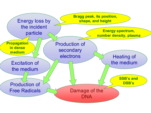
Figure 1: Schematics of the multi-scale approach.

As can be seen from this figure, propagation and stopping of incident ions in the tissue represent the initial stage of the whole scenario of ion therapy. The ion penetration depth depends strongly on their initial kinetic energy. A sharp maximum in energy deposition close to the end of their range is called a Bragg peak. Many works devoted to calculation of the exact location and shape of this peak include both deterministic and Monte-Carlo methods, see e.g., Ref.Pshen and references therein. Using the information about cross sections of atomic processes (such as ionization of water molecules) and nuclear processes (such as nuclear fragmentation of projectiles) as an input, these models give very good predictions of all characteristics of the Bragg peak, its position, height, tail, etc. These models provide reasonable information on the energy deposition on a mesoscopic scale of about 0.1 mm, which is sufficient for the treatment planning. The kinetic energy of ions changes from the initial energy in the range of 200-430 MeV/u down to about 50 keV/u. In our works nimb ; epjd , we presented a simple approach based on the singly differential cross section (SDCS) of ionization of a medium. In Ref. nimb , we have considered the ionization of water as a single process taking place on this scale, leaving other atomic interactions for later consideration. In Ref. epjd , we included the excitation of water molecules by projectiles. Even though no secondary electrons are produced in this process, it affects the energy loss and, therefore, the position of the Bragg peak; the excited water molecules are also prone to possess a higher probability for dissociation, leading to free radicals, H$\cdot$ and OH$\cdot$.

The next scale is defined by the secondary electrons and free radicals produced as a result of ionization and excitation of molecules of the medium. The maximum energy of electrons hardly exceeds 100 eV and their displacement is of the order of 10-15 nm. The main event on this scale is the diffusion of free electrons and radicals in the medium. They induce many chemical reactions which are important for the DNA damage since they define the agents interacting with the DNA. This aspect has been studied within several Monte Carlo models, see e.g. Nikjoo06 , which use various SDCS for ion and electron energy loss and include effects of the medium liqh2o ; Meesungnoen02 ; mfp ; Pimblott3 ). The propagation of electrons and other species through the medium is simulated explicitly until their interaction with the DNA. In this paper, we present another approach to describe this stage without using Monte Carlo simulations.

Interaction of electrons and radicals with DNA also happens on a nanometer scale, and many works are devoted to study these interactions DNA2 ; DNA3 ; Sanche05 ; DNA1 ; DNA4 ; DNA5 . In this work, we use the experimental results of Ref. DNA2 ; DNA3 ; Sanche05 .

The paper is organized as follows. In Section II we introduce the various phenomena defining scales involved in the process, ion stopping, propagation of secondary electrons and damage to DNA. In section III, we make some estimates of DNA damage caused by ions passing through glial cells using the results obtained in the previous chapters and biological data. A section of conclusions summarizes the paper.

II DNA damage as multi-scale process

II.1 Ion stopping and production of secondary electrons

Delta electrons play a major role in the energy loss by projectiles and therefore determine, to a large extent, all characteristics of the Bragg peak. Their energy spectrum, analyzed in our previous works nimb ; epjd , is important for the DNA damage calculations (see below).

Physically, the SDCS is determined by the properties of the medium, and since we use liquid water as a substitute for biological tissue, it is determined by the properties of water molecules and the properties of liquid water as a continuous medium. This information is contained in the real and imaginary parts of the electric susceptibility of liquid water. This approach can be generalized for any real tissue if the quantities, such as SDCS, for this medium are known.

In Refs. nimb ; epjd , we have used for the SDCS a semi-empirical parametrization by Rudd Rudd92 and obtained the position of the Bragg peak with a less than 3% discrepancy as compared to Monte Carlo simulations and experimental data epjd . These calculations are not very sensitive to the exact form of the SDCS, since the Linear Energy Transfer (LET) is determined after integration over the energy of the secondary electrons, $W$; however, the calculations of the DNA damage may be more sensitive to the shape of the SDCS at small energies, which for liquid water is different from that of water vapor Pimblott ; Pimblott2 ; Dingfelder ; Garcia .

The SDCS is a function of the projectile’s velocity and, since the ions are quite fast in the beginning of their trajectory, it has to be treated relativistically. In Ref. epjd , this issue has been solved by “relativization” of the Rudd parametrization by fitting it to correct Bethe asymptotic behavior in the relativistic limit.

Another important issue related to SDCS is the effect of charge transfer, due to pick-up electrons by the initially fully stripped ions (such as ¹²C⁶⁺) as they slow down in the medium. Since the SDCS is proportional to the square of ion charge, its reduction strongly influences such characteristics as the height of the Bragg peak, secondary electron abundance, etc. In Ref. epjd , we solved this problem by introducing an effective charge taken from Barkas63 . As a result, the effective charge of the ¹²C⁶⁺ near the Bragg peak is about $+3$ rather than $+6$.

Even after the relativistic treatment of the projectile and the introduction of effective charge, the profile of the Bragg peak obtained in our calculations was substantially higher and narrower than those obtained by Monte Carlo simulations or experiments. The main reason for the discrepancy was that our calculations were performed for a single unscattered ion, while in simulations, as well as in experiments, the ultimate results are a combination of many ion tracks with a significant spread in energy and position due to multiple scattering by water molecules. After we took into account straggling of the ions, the shape of our Bragg peak matched the shape predicted by the Monte Carlo simulations with nuclear fragmentation channels blocked RADAM2 .

The nuclear fragmentation in the case of carbon ions is quite substantial and should not be neglected. In principle, we can include the beam attenuation due to nuclear reactions given the energy dependent cross sections of these reactions, as we showed in Ref. RADAM2 . Then we would reproduce the attenuation of the ion beam , secondary electron production due to different species, the spread of the Bragg peak due to different penetration depths of different species, and the tail following the Bragg peak due to light products such as protons and neutrons. All these complications, however, were beyond our primary goal of gathering the most significant effects. We leave this to future refining calculations. We should mention that a successful treatment of nuclear processes has been done by the GEANT4 based Monte Carlo simulations Pshen .

Thus, the ionization energy loss by ions in liquid water is the dominating process for ion stopping and the energy spectrum of the secondary electrons. Additional energy losses are associated with the excitation of water molecules leading to the production of free radicals. The SDCS defines both the longest (in distance) scale related to the ion energy loss and provides the initial conditions for the next scale related to the propagation of the secondaries.

II.2 Propagation of secondary electrons

Even though the SDCS that we have used in epjd was not ideal, it does give some important predictions, which agree quite well with other calculations and measurements. Indeed, the average energy of the secondary electrons,

$$\left\langle W\right\rangle=\frac{1}{\sigma_{\rm T}}\int_{0}^{\infty}W\frac{d\sigma(W,T)}{dW}dW~{},$$ (1)

in the vicinity of the Bragg peak ($T\approx 0.3$ MeV/u) is about 45 eV. This value constrains possible further processes with such electrons. For instance, it has been shown that such electrons may excite or ionize another water molecule, but, most likely, only once, and the next generation of electrons is hardly capable of ionizing water molecules nimb ; epjd . This puts a limit on the number of secondary electrons produced.

The secondary electrons propagate in the same medium as the ion, and interaction with the medium is again determined by the SDCS with electrons being projectiles. The interaction can be elastic or inelastic, and there is a probability that it will interact with a DNA molecule and cause damage.

The angular distribution of the secondary electrons at energies about and below 45 eV is rather flat angle . Therefore, to a first approximation, we can consider Brownian motion of secondary electrons and use a random walk to describe their propagation through the medium from the point of production. The probability density to diffuse through a distance $r$ after $k$ steps is given by expression Chandra

$$P(k,r)=\frac{1}{\left(\frac{2\pi kl^{2}}{3}\right)^{3/2}}\exp\left(-\frac{3r^{2}}{2kl^{2}}\right)~{},$$ (2)

where the mean free path $l$ is the average distance that is traversed by the electron between two consecutive elastic collisions. It is determined by the elastic SDCS for electrons as projectiles and we use the results of Ref. mfp . Typical values for this mean free path (for the energies of interest) are about 0.3 nm The mean free path for inelastic collisions $l_{in}$ is typically about 20 times longer. So, we assume that electrons mainly experience elastic collisions and inelastic processes are included via an attenuation factor

$$\epsilon(k,W)=\mathcal{N}^{-1}\exp\left(-lk/l_{in}\right)~{},$$ (3)

corresponding to an average distance wandered $kl$; and where $\mathcal{N}=\int_{1}^{\infty}\epsilon dk=\exp\left(-l/l_{in}\right)/\left(l/l_{in}\right)$, is a normalization factor, since (3) provides the distribution over the number of steps. Both elastic and inelastic mean free paths depend on the energy of the wandering electron. This energy is changing gradually (with a number of steps), and strictly speaking, the mean free path is a function of the initial energy and the number of steps. The energies of secondary electrons are typically between 5 and 100 eV , and their average energy near the Bragg peak is 45 eV. The simulations of Ref. Meesungnoen02 suggest that the maximum range of displacement of such electrons is almost independent of their initial energy. This leads us to a model where we assume that all electrons are produced at some average energy and diffuse with the corresponding mean free paths, $l$ and $l_{in}$, which do not change during the diffusion.

As shown in Refs. nimb ; epjd , the number of these electrons produced per segment of an ion’s track, $d\zeta$, is given by $\frac{d^{2}N}{dWd\zeta}\Delta W$. This quantity is proportional to the SDCS of ionization by the projectiles. It depends on their kinetic energy and, therefore, on the depth in the tissue. For the calculations in this work we used the values from Ref. epjd in the vicinity of the Bragg peak, i.e., at an ion energy $T=0.3$ MeV/u. In this work, we assume the energy of electrons to be 20 eV, i.e., 25 eV lower than the average energy of secondary electrons, and took all of them, i.e., integrated $\frac{d^{2}N}{dWd\zeta}$ at $T=0.3$ eV from Ref. epjd over $W$ from 6 to 100 eV. This gives us $\frac{dN}{d\zeta}=8.8$ nm^-1. The reason for choosing 20-eV electrons is an analysis of the behavior of mean free paths mfp . It turns out that if the energy of secondary electrons is closer to 40 eV or higher, their inelastic mean free path, $l_{in}$, decreases. This means that they quickly lose energy to the value of about 20 eV, at which the ratio $l_{in}/l=20.2$. Otherwise, it would be difficult to interpret the results of Ref. Meesungnoen02 .

II.3 Evaluation of DNA damage

DNA damage, such as a Single Strand Break, is a result of a sequence of mutually independent events. First, a secondary electron with a certain kinetic energy $W$ is produced at a certain depth $x$. Then, this electron wanders in a surrounding medium interacting with its molecules elastically and inelastically gradually losing energy until it becomes bound. Depending on the electron’s energy, momentum and position, there is a chance that the electron stumbles on a DNA molecule and damages it. Following this scenario, we design a model for calculating the probability of a SSB due to a passing ion.

We consider the secondary electrons produced by an ion traversing the medium at a certain distance from the DNA and then let them wander toward a single convolution of the DNA. We represent this convolution of the DNA molecule by a cylinder of length 3.4 nm and radius 1.1 nm (these parameters are well established experimentally). We are interested in calculating the number of electrons hitting a single convolution because the DSB’s are defined as simultaneous breaks of both DNA strands located within a single convolution. Then, knowing the number of these electrons and their energy distribution, we can calculate the probability of damage to this convolution. If we can further assume a certain distribution (in space) of other convolutions, we can then calculate the total damage to the DNA molecule by averaging over all possible arrangements of convolutions with respect to the ion track.

The geometrical picture of an arbitrary ion track and a chosen convolution is schematically shown in Fig. 2, where geometrical notations are also included.

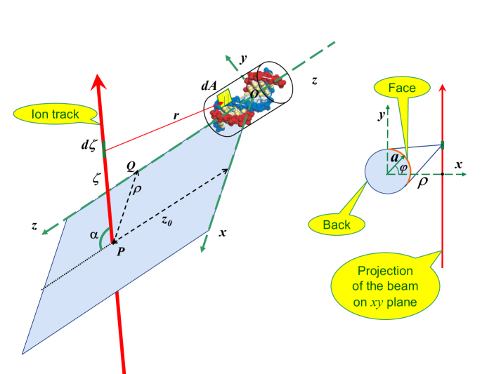
Figure 2: Geometry of the model: $z$ is the cylindrical axis of the DNA convolution and $x$ is chosen to be parallel to $PQ$, i.e., the line of closest approach between $z$ and the beam (orthogonal to both), of length $\rho$, at distance $z_{0}$ from the center of the convolution $O$. $\zeta$ is the coordinate of any point in the beam with respect to $P$, and $\alpha$ is the angle between the beam and $z$. In the right panel we show a projection on the $xy$ plane, where $a=1.1$ nm is the DNA radius and $\varphi$ is the polar angle defining a point on its surface.

From this scheme, it stems that any distance $r$ between a point on the track and a point on the cylinder is given by

$$r^{2}=(a\cos\varphi-\rho)^{2}+(a\sin\varphi-\zeta\sin\alpha)^{2}+(z-z_{0}-\zeta\cos\alpha)^{2}~{}.$$ (4)

Given a number of electrons produced within a segment $d\zeta$, we need to calculate the flux of these electrons through an area $d{\vec{A}}$ of the cylinder separated by a distance $r$ from the segment. Assuming Brownian diffusion of the electrons, the probability for one electron to diffuse from the ion track through the distance $r$ (after $k$ steps) is $P(k,r)d{\vec{r}}$.

Then the flux through a “patch”, $d{\vec{A}}$, of the cylinder is given by

$$d\Phi_{k}(r,W;W_{f})=d{\vec{A}}\cdot D\nabla P(k,r)\frac{d^{2}N}{dWd\zeta}(\zeta,W)\Delta W=d{\vec{A}}\cdot D\nabla P(k,r)\epsilon(k,W)\frac{dN}{d\zeta}(\zeta)~{},$$ (5)

where $D=kl^{2}/6$ is the diffusion coefficient multiplied by the average time of wandering, and $\epsilon(k,W)$ is defined in Eq. (3).

Finally, we assume that the number of the SSB’s within the DNA cylinder is proportional to the number of electrons crossing its surface, regardless of whether they are going into or leaving the cylinder. This number is proportional to the integral of the absolute value of the flux, i.e.,

$$N_{SSB}=\Gamma_{SSB}(W)\sum_{k}\int d\zeta d\Phi_{k}(r,W;W_{f})~{},$$ (6)

where the integrations are done over the surface of cylinder and the ion trajectory, and summation is done over the number of steps. The unknown quantity $\Gamma_{SSB}(W)$, that for the moment we assume to be a constant ($\Gamma_{SSB}(W)=5\times 10^{-4}$), is determined from the experimental data of Refs. DNA2 ; DNA3 ; Sanche05 , where SSB’s and DSB’s were induced by 0.1–30-eV electron beams.

The calculation for the general case, as shown in Fig. 2, depends on three geometrical parameters that define the position and orientation of the DNA convolution with respect to the ion track, the distances $\rho$ and $z_{0}$ and the angle $\alpha$. In order to interpret these results, we set $z_{0}$ to zero, and consider separately two limiting cases, the “parallel” case when $\alpha=0$, and the “normal” case when $\alpha=\pi/2$. In the parallel case, the cylinder containing the DNA convolution is parallel to the ion track and $\rho$ is the distance between the axis of the cylinder and the track. In the normal case, the axis of this cylinder is perpendicular to the ion track and when $z_{0}=0$, $\rho$ is again the distance between the axis of the cylinder and the track. In the latter case the beam projects along $\rho$ to the center of the cylinder. In both these cases, we need to set the limits for the angular integration over $\varphi$.

Looking from any point on the ion track, there are two surfaces of the DNA cylinder: the “front” or “face” surface and the “back” surface (see Fig. 2). In our model, if a wandering electron hits the face or the back surface, it may cause a strand break with a certain probability. Therefore, we simply add the probability of a SSB due to electrons striking the back surface to that for the face surface, regardless of the directions of their motion, leaving out the introduction of an attenuation mechanism to account for an electron passage “through the DNA” for a future extension of this model.

The results of the integration are shown in Fig. 3.

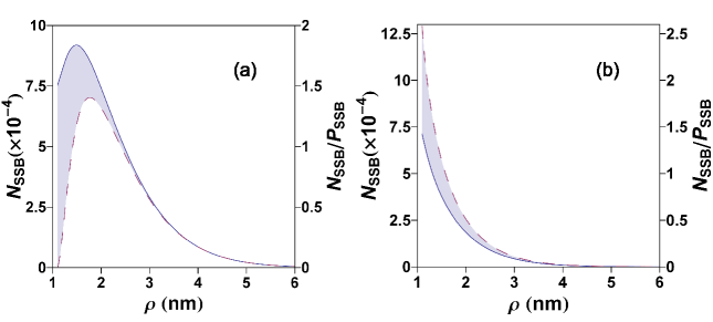
Figure 3: A comparison of numbers of SSB’s for parallel (dashed line) and normal (solid line) configurations on the face (a) and on the back side (b) for 20-eV electrons.

All curves show the dependence on the distance $\rho$ from the DNA to the beam. When the distance is large enough ($>3$ nm) the normal and parallel cases coincide for the face side as well as for the back side; differences appear only at small distances. These differences are significant only for back and face sides taken separately, but not for their combination shown in Fig. 4a.

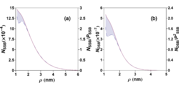
Figure 4: A comparison of dependencies of overall (due to the whole surface of the cylinder) SSB’s (a) and DSB’s due to separate electrons (b) on distances to the DNA convolution in the parallel (dashed line) and normal (solid line) cases for 20-eV electrons.

This means that the geometrical details of the orientation of DNA segments with respect to the beam may not be so significant, since all variations lie somewhere in the shadowed region in Fig. 4a, i.e., between the two curves. For a more general picture, some average curve (lying between the two curves in Fig. 4) should be used, with $\rho^{2}$ replaced by $\rho^{2}+z_{0}^{2}$. The numbers of SSB’s caused by the secondary electrons depending on the distance $\rho$ and the energy of the secondary electrons for the parallel case are shown in Fig. 5.

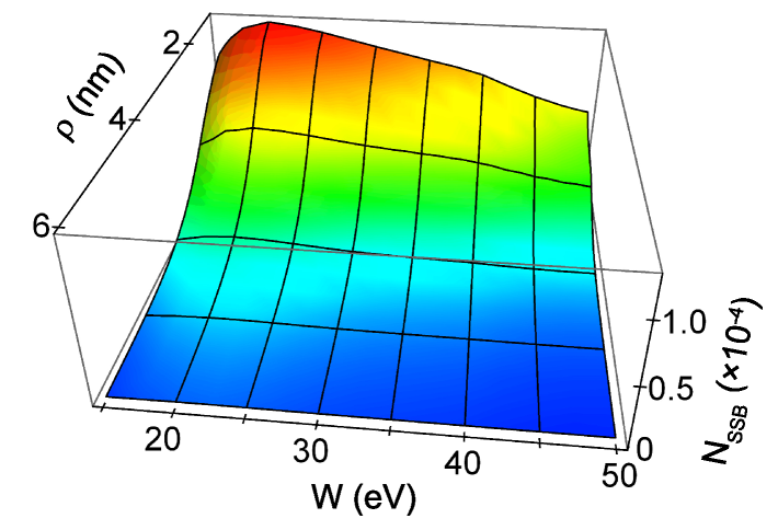
Figure 5: The number of SSB’s as a function of the distance to the DNA convolution, $\rho$, and the energy of secondary electrons (parallel case).

The decline of the number of SSB’s with increasing $\rho$ is an explicit consequence of Eqs. (2) and (4). The energy dependence is mainly caused by the dependence of the mean free paths on the energy and the attenuation factor given in Eq. (3). This factor is heuristic and may have to be corrected later when the corresponding experimental or computational data are available. This figure corresponds to our model, which includes the dependence of the mean free paths on the initial energy of secondary electrons, but assumes that the mean free paths do not change during the diffusion.

Generally, the DSB may be caused either by a single electron, if its energy is high enough, or by two different electrons, if the electron density is high enough. From Refs. DNA2 ; DNA3 ; Sanche05 , it follows that the DSB’s caused by the electrons with energies higher than about 5 eV happen in one hit, i.e., if a particular electron with a probability of about 0.0005 causes a SSB, the same electron causes a DSB with a probability of about 0.2 of the probability of the SSB (so the overall probability of a DSB is about $10^{-4}$ rather than $10^{-7}$. This is why the analysis of the probabilities of SSB’s is so important. If the energy of the secondaries are high enough they give the probability of DSB’s after being divided by some factor (about 5). Therefore, Fig. 5 also gives the shape of the dependence of DSB’s on distance and energy.

At energies lower than 5 eV the situation changes; one electron can not produce two breaks alone. Therefore, we need to calculate the number of DSB’s caused by two different electrons. From the geometry of a DNA convolution we infer that the probability of a DSB is proportional to $\frac{1}{4}(N_{SSB,face}^{2}+N_{SSB,back}^{2})+\frac{1}{2}N_{SSB,face}N_{SSB,back}$. This factor accounts for the probability of the occurrence of a SSB on the face for one strand, accompanied by a SSB on the other strand occurring either on the face or on the back, plus the probability of the inverse event. The numbers for the DSB’s caused by different electrons in parallel and normal cases are shown in Fig. 4b. Similar to the case of SSB’s, the differences due to geometry are not very significant. Even though the numbers of DSB’s plotted in Fig. 4b are many times smaller than those in Fig. 4a, this effect may be significant if the density of secondary electrons is large enough. According to our estimates in Refs. nimb ; epjd , the density of the secondary electrons produced by carbon ions at therapeutic energies in the vicinity of the Bragg peak is by about 16 orders of magnitude higher than the electron density in experiments of Ref. DNA2 ; DNA3 ; Sanche05 . Therefore, the two-electron mechanism of DSB formation may be the dominant channel.

This concludes our approach to calculations of DSB’s and SSB’s due to secondary electrons produced by ions. In the following subsection we’ll analyze the next generation of secondaries produced by electrons and free radicals produced by the ions.

II.4 Other secondaries

Secondary particles, which can be treated in a similar way as the secondary electrons are OH$\cdot$ radicals. They are formed as a result of the ionization of water molecules by an ion after dissociation of a water ion into OH$\cdot$ and H⁺. These radicals are formed almost at the same place as the secondary electrons. The difference is, of course, a different diffusion coefficient, and a different time of getting to the DNA, which is by about 100 times longer than that for secondary electrons. Then, the DNA damage caused by OH$\cdot$ may also be different sonntag ; geront . Nonetheless, if the effect produced by OH$\cdot$ is important, this is an argument for its inclusion into the model. The same can be said about those free radicals that are formed as a result of excitation of water molecules by ions. These radicals (OH$\cdot$ and H$\cdot$) are also produced in the ion track and can be treated in a similar way as secondary electrons.

Other secondaries, such as the second generation of electrons produced by the first generation via ionization of water, radicals produced as a result of this process and the radicals H$\cdot$ produced via interaction of secondary electrons with water molecules (e.g., through dissociative attachment) can be treated in the following way. Let the interaction that produces a “desired agent” happen at some point ${\vec{r}^{\prime}}$. Then the previous procedure has to be divided into three parts: diffusion of the secondary electron from the point of origin (the ion’s trajectory) to ${\vec{r}^{\prime}}$, an interaction that leads to the production of the agent at ${\vec{r}^{\prime}}$, and the diffusion of the agent to the DNA cylinder. Then, integration over ${\vec{r}^{\prime}}$ has to be performed.

III Calculation of lesion density along the track

We have established the way to calculate the probability of an SSB or a DSB at a DNA convolution at a certain distance from the ion path. Now a question is how many convolutions are there at different distances from the ion track. If we answer this question, we can predict the total amount of SSB’s and DSB’s caused by a single ion.

In order to answer this question, we have to accept a certain model for the tissue that is being irradiated. Let us consider glial cells in the mediodorsal thalamic nucleus as a target. Glial cells comprise 90% of the human brain and those of mediodorsal thalamic nucleus have been studied experimentally sz1 . These studies have provided the measurements of glial cell density as well as the size of their nuclei vital for our calculations.

Our calculations in the previous section are done for ions in the vicinity of the Bragg peak. The effective length along the ion track relevant for a single convolution is several nanometers, while the width of the Bragg peak is about 1 mm. Therefore, for the first estimate we can assume the probability of DSB’s to be constant if the distance from the ion track to the DNA convolution is between zero and $\rho_{0}\approx 10$ nm and zero at larger distances. Then, we can consider a cylinder of radius $\rho_{0}$ and length of $L=1$ mm surrounding a track of the ion traveling through the brain tissue. According to Ref. sz1 , the density of glial cells is $n_{cell}\approx 4.5\times 10^{-4}$ cells/$\mu$m³, the characteristic cell size is $s_{c}=n_{cell}^{-1/3}\approx 13\mu$m and the volume of a cell nucleus is $v_{nucl}\approx 140~{}\mu$m³ (approximate diameter of a nucleus $s_{n}\approx 5.2\mu$m). Therefore, the relative volume “filled” by the cell nuclei is equal to $v_{nucl}\times n_{cell}=0.063$, and the ion moving along this cylinder passes through $Ln_{cell}^{1/3}\approx 75$ cells.

If glial cells are in the interphase, i.e., the state of the cell cycle in which the cell exists most of its time, we can in the first approximation assume that the DNA is uniformly distributed inside the cell nucleus. Each DNA molecule has about $6\times 10^{8}$ convolutions, therefore the average convolution density inside an interphase nucleus is $n_{conv}=6\times 10^{8}/v_{nucl}=4.3\times 10^{6}$ convolutions/$\mu$m³.

Now we have to determine the probability of a DSB, $P_{DSB}$, assuming that they are made by single electrons of sufficient energy. From Fig. 4a, we can take the value of $P_{SSB}=1.25\times 10^{-3}$, corresponding to some average geometry, and divide it by a factor of 5 to get a value of $0.25\times 10^{-3}$ corresponding to probability of a DSB (due to the same electron). This value is obtained for liquid water. This medium may describe reasonably well the macroscopic quantities such as a Bragg peak position, which rely on a high percentage of water in the tissue. Yet, in the case we are now considering, the projectile is moving through a cell’s nucleus and the secondary electrons over this distance are produced by ionization of its molecules, which are not only water but also in DNA and RNA bases, sugars, etc., in not negligible quantities. Strictly speaking, we should recalculate all cross sections corresponding to the constituents of the cell nucleus, but for our estimate we will take the data from Ref. Terrissol , which suggest that these cross sections are about factor of 20 higher than that for water. Therefore, considering an estimation for the ratio of the volume occupied by these molecules in a nucleus, $v_{chromatine}/v_{nucl}\approx$ 50% volratio , we can combine these cross sections with the proper weight, obtaining $P_{DSB}=0.25\times 10^{-3}\times(20\times 0.5+0.5)=2.5\times 10^{-3}$.

Hence, if the ion is traveling through a cell nucleus, the density of DSB’s that it causes is equal to the $P_{DSB}\times n_{conv}\times\pi\rho^{2}\approx 2.5\times 10^{-3}\times 4.3\times 10^{6}\pi\times 0.01^{2}=$ 3.3 DSB/$\mu$m. This is comparable to the observations by Jacob et al. Jacob on human fibroblasts, where, at the energy deposition of about 1 Gy (=J/kg), the lesion density was found to be 4 DSB/$\mu$m in a nucleus.

Thus, we estimate that each ion in the vicinity of the Bragg Peak touches 75 cells, that is $75\times\frac{s_{n}^{2}}{s_{c}^{2}}=12$ nuclei, and inside each of these nuclei, about $3.3\times s_{n}=17.2$ DSB’s. If a cell is not in the interphase, but rather going through mitosis, then the DNA molecule is much more compact. Chromosomes rather than cell nuclei become targets for the secondary electrons. The volume of a chromosome is about 1.7 $\mu$m³, which increases the DNA convolution density to $3.5\times 10^{8}$ convolutions/$\mu$m³, but reduces the effective volume amenable to damage as well as the portion of the volume occupied by molecules different by water, thus affecting the cross sections. Then the number of DSB’s per cell will be about 0.5 if we use the same logic as above.

IV conclusions

Thus we presented a multi-scale approach to describe the physics relevant to ion-beam cancer therapy. We intend to present a clear physical picture of the events starting from an energetic ion entering the tissue and finally leading to DNA damage as a result of this incidence. We view this scenario as a palette of different phenomena that happen at different time, energy, and spatial scales. From this palette, we choose the processes that adequately describe the leading effects and then describe ways to include more details. We think that calculations in this field can be made inclusively without dwelling on a particular time or spatial scale. Our calculations are physically motivated, time effective and can provide reasonable accuracy. They show that the seemingly insurmountable complexity of the geometry of the DNA in different states may be tackled efficiently because the geometrical differences, shown in Fig. 4, are insignificant. We made the first estimate of the amount of DSB’s caused by an ion passing through glial cells and thus demonstrated the strength of this approach. We would like to encourage experimentalists to provide data more relevant to the actual conditions of irradiation, especially on the smallest scales involving DNA damage. This information is vital for further tuning of our approach by selecting and elaborating on the most important aspects of the problem.

- (1) U. Amaldi, G. Kraft, Rep. Prog. Phys. 68, 1861 (2005).
- (2) H. Tsujii et al., New J. Phys. 10, 075009 (2008).
- (3) O.I. Obolensky, E. Surdutovich, I. Pshenichnov, I. Mishustin, A. V. Solov’yov, and W. Greiner, Nucl. Inst. Meth. B 266, 1623–1628 (2008).
- (4) E. Surdutovich, O.I. Obolensky, E. Scifoni, I. Pshenichnov, I. Mishustin, A.V. Solov’yov, and W. Greiner, Eur. Phys. J. D, (to be published).
- (5) I. Pshenichnov, I. Mishustin, W. Greiner, Nucl. Inst. Meth. B 266, 1094–1098 (2008).
- (6) H. Nikjoo, S. Uehara, D. Emfietzoglou, F. A. Cucinotta, Radiat. Meas. 41, 1052 (2006).
- (7) M. Dingfelder, R.H. Ritchie, J.E. Turner, W. Friedland, H.G. Paretzke and R.N. Hamm, Radiat. Res. 169, 584–594 (2008).
- (8) J. Meesungnoen, J.-P. Jay-Gerin, A. Filali-Mouhim, S. Mankhetkorn, Radiat. Res. 158, 657 (2002).
- (9) C.J. Tung, T.C. Chao, H.W. Hsieh, W.T. Chan, Nucl. Inst. Meth B 262, 231–239 (2007).
- (10) S.M. Pimblott, J.A. LaVerne, and A. Mozumder, J. Phys. Chem 100, 8595–8606 (1996).
- (11) B. Boudaïffa, P. Cloutier, D. Hunting, M. A. Huels, L. Sanche, Science 287, 1658 (2000).
- (12) M. A. Huels, B. Boudaïffa, P. Cloutier, D. Hunting, L. Sanche, JACS 125, 4467 (2003).
- (13) L. Sanche, Eur. Phys. J. D 35, 367–390 (2005).
- (14) T.M. Orlando, D. Oh, Y. Chen, and A.B. Aleksandrov, J. Chem. Phys., 128, 195102 (2008).
- (15) W. Friedland, P. Jacob, P. Bernhardt, H.G. Paretzke, M. Dingfelder, Radiat. Res. 159, 401–410 (2003).
- (16) H. Nikjoo, C.E. Bolton, R. Watanabe, M. Terrisol, P.O’Neill and D.T. Goodhead, Radiat. Prot. Dosim. 99, 77-80 (2002).
- (17) M. E. Rudd, Y.-K. Kim, D. H. Madison, T. Gay, Rev. Mod. Phys. 64, 441 (1992).
- (18) S.M. Pimblott, J.A. LaVerne, Rad. Phys. Chem. 76, 1244-1247 (2007).
- (19) S.M. Pimblott, L.D.A. Siebbeles, Nucl. Inst. Meth. B 194, 237–250 (2002).
- (20) M. Dingfelder, D. Hantke, M. Inokuti, H.G. Paretzke, Radiat. Phys. Chem. 53, 1–18 (1998).
- (21) A. Munõz, F. Blanco, G. Garcia, P.A. Thorn, M.J. Brunger, J.P. Sullivan, S.J. Buckman, Int. J. Mass Spectrom., (to be published).
- (22) W.H. Barkas, Nuclear Research Emulsions I. Techniques and Theory, Academic Press Inc., New York, London, 1963, Vol. 1, 371.
- (23) E. Scifoni, E. Surdutovich, A.V. Solov’yov, I. Pshenichnov, I. Mishustin, and W. Greiner, AIP Conference Ser. (to be published).
- (24) W.E. Wilson, H. Nikjoo, Radiat. Environ. Biophys. 38, 97–104 (1999).
- (25) S. Chandrasekhar, Rev. Mod. Phys. 15, 1, (1943).
- (26) C. Sonntag, “Free-Radical-Induced DNA Damage as Approached by Quantum-Mechanical and Monte Carlo Calculations: An Overview from the Standpoint of an Experimentalist” in Advances in Quantum Chem.52, E. Brändas and J.R. Sabin, Elsevier, 2006, pp. 5–20.
- (27) C. Chatgilialoglu, P. O’Neil, Exp. Geront. 36, 1459–1471 (2001).
- (28) G. Chana, S. Landau, D. Cotter, Schizoph. Res., 102, 344 (2008).
- (29) S. Edel, M. Terrissol, A. Peudon, E. Kummerle, E. Pomplun, Rad. Protect. Dosim. 122, 136–140 (2006).
- (30) G. Lopez-Velazquez et al. , Histochem. Cell. Biol. 105, 153–161 (2006).
- (31) B. Jacob, M. Scholz, and G. Taucher-Scholz., Radiat. Res. 159, 676–684 (2003).