Spectrum of large random reversible Markov chains:
two examples

Abstract.

We take on a Random Matrix theory viewpoint to study the spectrum of certain reversible Markov chains in random environment. As the number of states tends to infinity, we consider the global behavior of the spectrum, and the local behavior at the edge, including the so called spectral gap. Results are obtained for two simple models with distinct limiting features. The first model is built on the complete graph while the second is a birth-and-death dynamics. Both models give rise to random matrices with non independent entries.

1. Introduction

The spectral analysis of large dimensional random matrices is a very active domain of research, connected to a remarkable number of areas of Mathematics, see e.g. [27, 22, 3, 10, 1, 37]. On the other hand, it is well known that the spectrum of reversible Markov chains provides useful information on their trend to equilibrium, see e.g. [31, 15, 29, 25]. The aim of this paper is to explore potentially fruitful links between the Random Matrix and the Markov Chains literature, by studying the spectrum of reversible Markov chains with large finite state space in a frozen random environment. The latter is obtained by assigning random weights to the edges of a finite graph. This approach raises a collection of stimulating problems, lying at the interface between Random Matrix theory, Random Walks in Random Environment, and Random Graphs. We focus here on two elementary models with totally different scalings and limiting objects: a complete graph model and a chain graph model. The study of spectral aspects of random Markov chains or random walks in random environment is not new, see for instance [18, 9, 39, 14, 13, 11, 34] and references therein. Here we adopt a Random Matrix theory point of view.

Consider a finite connected undirected graph $G=(V,E)$, with vertex set $V$ and edge set $E$, together with a set of weights, given by nonnegative random variables

$$\mathbf{U}=\{U_{i,j};\{i,j\}\in E\}.$$

Since the graph $G$ is undirected we set $U_{i,j}=U_{j,i}$. On the network $(G,\mathbf{U})$, we consider the random walk in random environment with state space $V$ and transition probabilities

(1) $$K_{i,j}=\frac{U_{i,j}}{\rho_{i}}\quad\text{where}\quad\rho_{i}=\sum_{j:\{i,j\}\in E}U_{i,j}.$$

The Markov kernel $K$ is reversible with respect to the measure $\rho=\{\rho_{i}\,,\;i\in V\}$ in that

$$\rho_{i}K_{i,j}=\rho_{j}K_{j,i}$$

for all $i,j\in V$. When the variables $\mathbf{U}$ are all equal to a positive constant this is just the standard simple random walk on $G$, and $K-I$ is the associated Laplacian. If $\rho_{i_{0}}=0$ for some vertex $i_{0}$ then we set $K_{i_{0},j}=0$ for all $j\neq i_{0}$ and $K_{i_{0},i_{0}}=1$ ($i_{0}$ is then an isolated vertex).

The construction of reversible Markov kernels from graphs with weighted edges as in (1) is classical in the Markovian literature, see e.g. [15, 19]. As for the choice of the graph $G$, we shall work with the simplest cases, namely the complete graph or a one–dimensional chain graph. Before passing to the precise description of models and results, let us briefly recall some broad facts.

By labeling the $n=|V|$ vertices of $G$ and putting $K_{i,j}=0$ if $\{i,j\}\not\in E$, one has that $K$ is a random $n\times n$ Markov matrix. The entries of $K$ belong to $[0,1]$ and each row sums up to $1$. The spectrum of $K$ does not depend on the way we label $V$. In general, even if the random weights $\mathbf{U}$ are i.i.d. the random matrix $K$ has non–independent entries due to the normalizing sums $\rho_{i}$. Note that $K$ is in general non–symmetric, but by reversibility, it is symmetric w.r.t. the scalar product induced by $\rho$, and its spectrum $\sigma(K)$ is real. Moreover, $1\in\sigma(K)\subset[-1,+1]$, and it is convenient to denote the eigenvalues of $K$ by

$$-1\leq\lambda_{n}(K)\leq\cdots\leq\lambda_{1}(K)=1.$$

If the weights $U_{i,j}$ are all positive, then $K$ is irreducible, the eigenspace of the largest eigenvalue $1$ is one–dimensional and thus $\lambda_{2}(K)<1$. In this case $\rho_{i}$ is its unique invariant distribution, up to normalization. Moreover, since $K$ is reversible, the period of $K$ is $1$ (aperiodic case) or $2$, and this last case is equivalent to $\lambda_{n}(K)=-1$ (the spectrum of $K$ is in fact symmetric when $K$ has period $2$); see e.g. [32].

The bulk behavior of $\sigma(K)$ is studied via the Empirical Spectral Distribution (ESD)

$$\mu_{K}=\frac{1}{n}\sum_{k=1}^{n}\delta_{\lambda_{k}(K)}.$$

Since $K$ is Markov, its ESD contains probabilistic information on the corresponding random walk. Namely, the moments of the ESD $\mu_{K}$ satisfy, for any $\ell\in\mathds{Z}_{+}$

(2) $$\int_{-1}^{+1}\!x^{\ell}\mu_{K}(dx)=\frac{1}{n}\mathrm{Tr}(K^{\ell})=\frac{1}{n}\sum_{i\in V}r^{\mathbf{U}}_{\ell}(i)$$

where $r^{\mathbf{U}}_{\ell}(i)$ denotes the probability that the random walk on $(G,{\bf U})$ started at $i$ returns to $i$ after $\ell$ steps.

The edge behavior of $\sigma(K)$ corresponds to the extreme eigenvalues $\lambda_{2}(K)$ and $\lambda_{n}(K)$, or more generally, to the $k$–extreme eigenvalues $\lambda_{2}(K),\dots,\lambda_{k+1}(K)$ and $\lambda_{n}(K),\dots,\lambda_{n-k+1}(K)$. The geometric decay to the equilibrium measure $\rho$ of the continuous time random walk with semigroup ${(e^{t(K-I)})}_{t\geq 0}$ generated by $K-I$ is governed by the so called spectral gap

$$\mathrm{gap}(K-I)=1-\lambda_{2}(K).$$

In the aperiodic case, the relevant quantity for the discrete time random walk with kernel $K$ is

$$\varsigma(K)=1-\max_{\begin{subarray}{c}\lambda\in\sigma(K)\\ \lambda\neq 1\end{subarray}}|\lambda|=1-\max(-\lambda_{n}(K),\lambda_{2}(K))\,.$$

In that case, for any fixed value of $n$, we have $(K^{\ell})_{i,\cdot}\to\rho$ as $\ell\to\infty$, for every $1\leq i\leq n$. We refer to e.g. [31, 25] for more details.

Complete graph model

Here we set $V=\{1,\dots,n\}$ and $E=\{\{i,j\};i,j\in V\}$. Note that we have a loop at any vertex. The weights $U_{i,j}$, $1\leq i\leq j\leq n$ are i.i.d. random variables with common law $\mathcal{L}$ supported on $[0,\infty)$. The law $\mathcal{L}$ is independent of $n$. Without loss of generality, we assume that the marks $\mathbf{U}$ come from the truncation of a single infinite triangular array $(U_{i,j})_{1\leq i\leq j}$ of i.i.d. random variables of law $\mathcal{L}$. This defines a common probability space, which is convenient for almost sure convergence as $n\to\infty$.

When $\mathcal{L}$ has finite mean $\int_{0}^{\infty}x\,\mathcal{L}(dx)=m$ we set $m=1$. This is no loss of generality since $K$ is invariant under the linear scaling $t\to t\,U_{i,j}$. If $\mathcal{L}$ has a finite second moment we write $\sigma^{2}=\int_{0}^{\infty}(x-1)^{2}\,\mathcal{L}(dx)$ for the variance. The rows of $K$ are equally distributed (but not independent) and follow an exchangeable law on $\mathds{R}^{n}$. Since each row sums up to one, we get by exchangeability that for every $1\leq i,j\neq j^{\prime}\leq n$,

$$\mathds{E}(K_{i,j})=\frac{1}{n}\quad\text{and}\quad\mathrm{Cov}(K_{i,j},K_{i,j^{\prime}})=-\frac{1}{n-1}\mathrm{Var}(K_{1,1}).$$

Note that $\mathcal{L}$ may have an atom at $0$, i.e. $\mathds{P}(U_{i,j}=0)=1-p$, for some $p\in(0,1)$. In this case $K$ describes a random walk on a weighted version of the standard Erdős-Rényi $G(n,p)$ random graph. Since $p$ is fixed, almost surely (for $n$ large enough) there is no isolated vertex, the row-sums $\rho_{i}$ are all positive, and $K$ is irreducible.

The following theorem states that if $\mathcal{L}$ has finite positive variance $0<\sigma^{2}<\infty$, then the bulk of the spectrum of $\sqrt{n}K$ behaves as if we had a Wigner matrix with i.i.d. entries, i.e. as if $\rho_{i}\equiv n$. We refer to e.g. [3, 1] for more on Wigner matrices and the semi–circle law. The ESD of $\sqrt{n}K$ is $\mu_{\sqrt{n}K}=\frac{1}{n}\sum_{k=1}^{n}\delta_{\sqrt{n}\lambda_{k}(K)}.$

Theorem 1.1 (Bulk behavior).

If $\mathcal{L}$ has finite positive variance $0<\sigma^{2}<\infty$ then

$$\mu_{\sqrt{n}K}\underset{n\to\infty}{\overset{w}{\longrightarrow}}\mathcal{W}_{2\sigma}$$

almost surely, where “$\overset{w}{\to}$” stands for weak convergence of probability measures and $\mathcal{W}_{2\sigma}$ is Wigner’s semi–circle law with Lebesgue density

(3) $$x\mapsto\frac{1}{2\pi\sigma^{2}}\sqrt{4\sigma^{2}-x^{2}}\,\,\mathds{1}_{\left[-2\sigma,+2\sigma\right]}(x)\,.$$

The proof of Theorem 1.1, given in Section 2, relies on a uniform strong law of large numbers which allows to estimate $\rho_{i}=n(1+o(1))$ and therefore yields a comparison of $\sqrt{n}K$ with a suitable Wigner matrix with i.i.d.  entries. Note that, even though

(4) $$\lambda_{1}(\sqrt{n}K)=\sqrt{n}\to\infty\quad\text{as}\quad n\to\infty,$$

the weak limit of $\mu_{\sqrt{n}K}$ is not affected since $\lambda_{1}(\sqrt{n}K)$ has weight $1/n$ in $\mu_{\sqrt{n}K}$. Theorem 1.1 implies that the bulk of $\sigma(K)$ collapses weakly at speed $n^{-1/2}$. Concerning the extremal eigenvalues $\lambda_{n}(\sqrt{n}K)$ and $\lambda_{2}(\sqrt{n}K)$, we only get from Theorem 1.1 that almost surely, for every fixed $k\in\mathds{Z}_{+}$,

$$\liminf_{n\to\infty}\sqrt{n}\lambda_{n-k}(K)\leq-2\sigma\quad\text{and}\quad\limsup_{n\to\infty}\sqrt{n}\lambda_{k+2}(K)\geq+2\sigma.$$

The result below gives the behavior of the extremal eigenvalues under the assumption that $\mathcal{L}$ has finite fourth moment (i.e. $\mathds{E}(U_{1,1}^{4})<\infty$).

Theorem 1.2 (Edge behavior).

If $\mathcal{L}$ has finite positive variance $0<\sigma^{2}<\infty$ and finite fourth moment then almost surely, for any fixed $k\in\mathds{Z}_{+}$,

$$\lim_{n\to\infty}\sqrt{n}\lambda_{n-k}(K)=-2\sigma\quad\text{and}\quad\lim_{n\to\infty}\sqrt{n}\lambda_{k+2}(K)=+2\sigma.$$

In particular, almost surely,

(5) $$\mathrm{gap}(K-I)=1-\frac{2\sigma}{\sqrt{n}}+o\left(\frac{1}{\sqrt{n}}\right)\quad\text{and}\quad\varsigma(K)=1-\frac{2\sigma}{\sqrt{n}}+o\left(\frac{1}{\sqrt{n}}\right).$$

The proof of Theorem 1.2, given in Section 2, relies on a suitable rank one reduction which allows us to compare $\lambda_{2}(\sqrt{n}K)$ with the largest eigenvalue of a Wigner matrix with centered entries. This approach also requires a refined version of the uniform law of large numbers used in the proof of Theorem 1.1.

The edge behavior of Theorem 1.2 allows one to reinforce Theorem 1.1 by providing convergence of moments. Recall that for any integer $p\geq 1$, the weak convergence together with the convergence of moments up to order $p$ is equivalent to the convergence in Wasserstein $W_{p}$ distance, see e.g. [36]. For every real $p\geq 1$, the Wasserstein distance $W_{p}(\mu,\nu)$ between two probability measures $\mu,\nu$ on $\mathds{R}$ is defined by

(6) $$W_{p}(\mu,\nu)=\inf_{\Pi}\left(\int_{\mathds{R}\times\mathds{R}}\!|x-y|^{p}\,\Pi(dx,dy)\right)^{1/p}$$

where the infimum runs over the convex set of probability measures on $\mathds{R}^{2}=\mathds{R}\times\mathds{R}$ with marginals $\mu$ and $\nu$. Let $\widetilde{\mu}_{\sqrt{n}K}$ be the trimmed ESD defined by

$$\widetilde{\mu}_{\sqrt{n}K}=\frac{1}{n-1}\sum_{k=2}^{n}\delta_{\sqrt{n}\lambda_{k}(K)}=\frac{n}{n-1}\mu_{\sqrt{n}K}-\frac{1}{n-1}\delta_{\sqrt{n}}.$$

We have then the following Corollary of theorems 1.1 and 1.2, proved in Section 2.

Corollary 1.3 (Strong convergence).

If $\mathcal{L}$ has positive variance and finite fourth moment then almost surely, for every $p\geq 1$,

$$\lim_{n\to\infty}W_{p}(\widetilde{\mu}_{\sqrt{n}K},\mathcal{W}_{2\sigma})=0\quad\text{while}\quad\lim_{n\to\infty}W_{p}(\mu_{\sqrt{n}K},\mathcal{W}_{2\sigma})=\begin{cases}0&\text{if $p<2$}\\ 1&\text{if $p=2$}\\ \infty&\text{if $p>2$}.\end{cases}$$

Recall that for every $k\in\mathds{Z}_{+}$, the $k^{\text{th}}$ moment of the semi–circle law $\mathcal{W}_{2\sigma}$ is zero if $k$ is odd and is $\sigma^{k}$ times the $(k/2)^{\text{th}}$ Catalan number if $k$ is even. The $r^{\text{th}}$ Catalan number $\frac{1}{r+1}\,\binom{2r}{r}$ counts, among other things, the number of non–negative simple paths of length $2r$ that start and end at $0$.

On the other hand, from (2), we know that for every $k\in\mathds{Z}_{+}$, the $k^{\text{th}}$ moment of the ESD $\mu_{\sqrt{n}K}$ writes

$$\int_{\mathds{R}}\!x^{k}\,\mu_{\sqrt{n}K}(dx)=\frac{1}{n}\,{\rm Tr}\left((\sqrt{n}K)^{k}\right)=n^{-1+\frac{k}{2}}\sum_{i=1}^{n}r^{\mathbf{U}}_{k}(i)\,.$$

Additionally, from (4) we get

$$\int_{\mathds{R}}\!x^{k}\,\mu_{\sqrt{n}K}(dx)=n^{-1+\frac{k}{2}}+\left(1-\frac{1}{n}\right)\int_{\mathds{R}}\!x^{k}\,\widetilde{\mu}_{\sqrt{n}K}(dx)$$

where $\widetilde{\mu}_{\sqrt{n}K}$ is the trimmed ESD defined earlier. We can then state the following.

Corollary 1.4 (Return probabilities).

Let $r^{\mathbf{U}}_{k}(i)$ be the probability that the random walk on $V$ with kernel $K$ started at $i$ returns to $i$ after $k$ steps. If $\mathcal{L}$ has variance $0<\sigma^{2}<\infty$ and finite fourth moment then almost surely, for every $k\in\mathds{Z}_{+}$,

(7) $$\lim_{n\to\infty}n^{-1+\frac{k}{2}}\left(\sum_{i=1}^{n}r^{\mathbf{U}}_{k}(i)-1\right)=\begin{cases}0&\text{if $k$ is odd}\\ \frac{\sigma^{k}}{k/2+1}\binom{k}{k/2}&\text{if $k$ is even}.\end{cases}$$

We end our analysis of the complete graph model with the behavior of the invariant probability distribution $\hat{\rho}$ of $K$, obtained by normalizing the invariant vector $\rho$ as

$$\hat{\rho}=(\rho_{1}+\cdots+\rho_{n})^{-1}(\rho_{1}\delta_{1}+\cdots+\rho_{n}\delta_{n}).$$

Let $\mathcal{U}=n^{-1}(\delta_{1}+\cdots+\delta_{n})$ denote the uniform law on $\{1,\ldots,n\}$. As usual, the total variation distance $\|\mu-\nu\|_{\textsc{tv}}$ between two probability measures $\mu=\sum_{k=1}^{n}\mu_{k}\delta_{k}$ and $\nu=\sum_{k=1}^{n}\nu_{k}\delta_{k}$ on $\{1,\ldots,n\}$ is given by

$$\|\mu-\nu\|_{\textsc{tv}}=\frac{1}{2}\sum_{k=1}^{n}|\mu_{k}-\nu_{k}|.$$

Proposition 1.5 (Invariant probability measure).

If $\mathcal{L}$ has finite second moment, then a.s.

(8) $$\lim_{n\to\infty}\|\hat{\rho}-\mathcal{U}\|_{\textsc{tv}}=0.$$

The proof of Proposition 1.5, given in Section 2, relies as before on a uniform law of large numbers. The speed of convergence and fluctuation of $\|\hat{\rho}-\mathcal{U}\|_{\textsc{tv}}$ depends on the tail of $\mathcal{L}$. The reader can find in Lemma 2.3 of Section 2 some estimates in this direction.

Chain graph model (birth-and-death)

The complete graph model discussed earlier provides a random reversible Markov kernel which is irreducible and aperiodic. One of the key feature of this model lies in the fact that the degree of each vertex is $n$, which goes to infinity as $n\to\infty$. This property allows one to use a law of large numbers to control the normalization $\rho_{i}$. The method will roughly still work if we replace the complete graphs sequence by a sequence of graphs for which the degrees are of order $n$. See e.g. [37] for a survey of related results in the context of random graphs. To go beyond this framework, it is natural to consider local models for which the degrees are uniformly bounded. We shall focus on a simple birth-and-death Markov kernel $K=(K_{i,j})_{1\leq i,j\leq n}$ on $\{1,\ldots,n\}$ given by

$$K_{i,i+1}=b_{i},\quad K_{i,i}=a_{i},\quad K_{i,i-1}=c_{i}$$

where $(a_{i})_{1\leq i\leq n}$, $(b_{i})_{1\leq i\leq n}$, $(c_{i})_{1\leq i\leq n}$ are in $[0,1]$ with $c_{1}=b_{n}=0$ , $b_{i}+a_{i}+c_{i}=1$ for every $1\leq i\leq n$, and $c_{i+1}>0$ and $b_{i}>0$ for every $1\leq i\leq n-1$. In other words, we have

(9) $$K=\begin{pmatrix}a_{1}&b_{1}\\ c_{2}&a_{2}&b_{2}\\ &c_{3}&a_{3}&b_{3}\\ &&\ddots&\ddots&\ddots\\ &&&c_{n-1}&a_{n-1}&b_{n-1}\\ &&&&c_{n}&a_{n}\end{pmatrix}.$$

The kernel $K$ is irreducible, reversible, and every vertex has degree $\leq 3$. For an arbitrary $\rho_{1}>0$, the measure $\rho=\rho_{1}\delta_{1}+\cdots+\rho_{n}\delta_{n}$ defined for every $2\leq i\leq n$ by

$$\rho_{i}=\rho_{1}\prod_{k=1}^{i-1}\frac{b_{k}}{c_{k+1}}=\rho_{1}\frac{b_{1}\cdots b_{i-1}}{c_{2}\cdots c_{i}}$$

is invariant and reversible for $K$, i.e. for $1\leq i,j\leq n$, $\rho_{i}K_{i,j}=\rho_{j}K_{j,i}.$ For every $1\leq i\leq n$, the $i^{\text{th}}$ row $(c_{i},a_{i},b_{i})$ of $K$ belongs to the $3$-dimensional simplex

$$\Lambda_{3}=\{v\in[0,1]^{3};v_{1}+v_{2}+v_{3}=1\}.$$

For every $v\in\Lambda_{3}$, we define the left and right “reflections” $v_{-}\in\Lambda_{3}$ and $v_{+}\in\Lambda_{3}$ of $v$ by

$$v_{-}=(v_{1}+v_{3},v_{2},0)\quad\text{and}\quad v_{+}=(0,v_{2},v_{1}+v_{3}).$$

The following result provides a general answer for the behavior of the bulk.

Theorem 1.6 (Global behavior for ergodic environment).

Let $\mathbf{p}:\mathds{Z}\to\Lambda_{3}$ be an ergodic random field. Let $K$ be the random birth-and-death kernel (9) on $\{1,\ldots,n\}$ obtained from $\mathbf{p}$ by taking for every $1\leq i\leq n$

$$(c_{i},a_{i},b_{i})=\begin{cases}\mathbf{p}(i)&\text{if $2\leq i\leq n-1$}\\ \mathbf{p}(1)_{+}&\text{if $i=1$}\\ \mathbf{p}(n)_{-}&\text{if $i=n$}.\end{cases}$$

Then there exists a non-random probability measure $\mu$ on $[-1,+1]$ such that almost surely,

$$\lim_{n\to\infty}W_{p}(\mu_{K},\mu)=0$$

for every $p\geq 1$, where $W_{p}$ is the Wasserstein distance (6). Moreover, for every $\ell\geq 0$,

$$\int_{-1}^{+1}\!x^{\ell}\,\mu(dx)=\mathds{E}[r^{\mathbf{p}}_{\ell}(0)]$$

where $r^{\mathbf{p}}_{\ell}(0)$ is the probability of return to $0$ in $\ell$ steps for the random walk on $\mathds{Z}$ with random environment $\mathbf{p}$. The expectation is taken with respect to the environment $\mathbf{p}$.

The proof of Theorem 1.6, given in Section 3, is a simple consequence of the ergodic theorem; see also [9] for an earlier application to random conductance models. The reflective boundary condition is not necessary for this result on the bulk of the spectrum, and essentially any boundary condition (e.g. Dirichlet or periodic) produces the same limiting law, with essentially the same proof. Moreover, this result is not limited to the one–dimensional random walks and it remains valid e.g. for any finite range reversible random walk with ergodic random environment on $\mathds{Z}^{d}$. However, as we shall see below, a more precise analysis is possible for certain type of environments when $d=1$.

Consider the chain graph $G=(V,E)$ with $V=\{1,\ldots,n\}$ and $E=\{(i,j);|i-j|\leq 1\}$. A random conductance model on this graph can be obtained by defining $K$ with (1) by putting i.i.d. positive weights $\mathbf{U}$ of law $\mathcal{L}$ on the edges. For instance, if we remove the loops, this corresponds to define $K$ by (9) with $a_{1}=\cdots=a_{n}=0$, $b_{1}=c_{n}=1$, and, for every $2\leq i\leq n-1$,

$$b_{i}=1-c_{i}=V_{i}=\frac{U_{i,i+1}}{U_{i,i+1}+U_{i,i-1}}.$$

where $(U_{i,i+1})_{i\geq 1}$ are i.i.d.  random variables of law $\mathcal{L}$ supported in $(0,\infty)$. The random variables $V_{1},\ldots,V_{n}$ are dependent here.

Let us consider now an alternative simple way to make $K$ random. Namely, we use a sequence $(V_{i})_{i\geq 1}$ of i.i.d. random variables on $[0,1]$ with common law $\mathcal{L}$ and define the random birth-and-death Markov kernel $K$ by (9) with

$$b_{1}=c_{n}=1\quad\text{and}\quad b_{i}=1-c_{i}=V_{i}\quad\text{for every $2\leq i\leq n-1$.}$$

In other words, the random Markov kernel $K$ is of the form

(10) $$K=\begin{pmatrix}0&1\\ 1-V_{2}&0&V_{2}\\ &1-V_{3}&0&V_{3}\\ &&\ddots&\ddots&\ddots\\ &&&1-V_{n-1}&0&V_{n-1}\\ &&&&1&0\end{pmatrix}.$$

This is not a random conductance model. However, the kernel is a particular case of the one appearing in Theorem 1.6, corresponding to the i.i.d. environment given by

$$\mathbf{p}(i)=(1-V_{i},0,V_{i})$$

for every $i\geq 1$. This gives the following corollary of Theorem 1.6.

Corollary 1.7 (Global behavior for i.i.d.  environment).

Let $K$ be the random birth-and-death Markov kernel (10) where $(V_{i})_{i\geq 2}$ are i.i.d.  of law $\mathcal{L}$ on $[0,1]$. Then there exists a non-random probability distribution $\mu$ on $[-1,+1]$ such that almost surely,

$$\lim_{n\to\infty}W_{p}(\mu_{K},\mu)=0$$

for every $p\geq 1$, where $W_{p}$ is the Wasserstein distance as in (6). The limiting spectral distribution $\mu$ is fully characterized by its sequence of moments, given for every $k\geq 1$ by

$$\int_{-1}^{+1}\!x^{2k-1}\,\mu(dx)=0\quad\text{ and }\quad\int_{-1}^{+1}\!x^{2k}\,\mu(dx)=\sum_{\gamma\in D_{k}}\prod_{i\in\mathds{Z}}\mathds{E}\left(V^{N_{\gamma}(i)}(1-V)^{N_{\gamma}(i-1)}\right)$$

where $V$ is a random variable of law $\mathcal{L}$ and where

$$D_{k}=\{\gamma=(\gamma_{0},\ldots,\gamma_{2k}):\gamma_{0}=\gamma_{2k}=0,\text{ and }|\gamma_{\ell}-\gamma_{\ell+1}|=1\text{ for every $0\leq\ell\leq 2k-1$}\}$$

is the set of loop paths of length $2k$ of the simple random walk on $\mathds{Z}$, and

$$N_{\gamma}(i)=\sum_{\ell=0}^{2k-1}\mathds{1}_{\{(\gamma_{\ell},\gamma_{\ell+1})=(i,i+1)\}}$$

is the number of times $\gamma$ crosses the horizontal line $y=i+\frac{1}{2}$ in the increasing direction.

When the random variables $(V_{i})_{i\geq 2}$ are only stationary and ergodic, Corollary 1.7 remains valid provided that we adapt the formula for the even moments of $\mu$ (that is, move the product inside the expectation).

Remark 1.8 (From Dirac masses to arc–sine laws).

Corollary 1.7 gives a formula for the moments of $\mu$. This formula is a series involving the “Beta-moments” of $\mathcal{L}$. We cannot compute it explicitly for arbitrary laws $\mathcal{L}$ on $[0,1]$. However, in the deterministic case $\mathcal{L}=\delta_{1/2}$, we have, for every integer $k\geq 1$,

$$\int_{-1}^{+1}\!x^{2k}\mu(dx)=\sum_{\gamma\in D_{k}}2^{-\sum_{i}N_{\gamma}(i)-\sum_{i}N_{\gamma}(i-1)}=2^{-2k}{\binom{2k}{k}}=\int_{-1}^{+1}\!\!x^{2k}\frac{dx}{\pi\sqrt{1-x^{2}}}$$

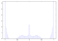
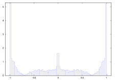
Figure 1. Plots illustrating Corollary 1.7. Each histogram corresponds to the spectrum of a single realization of $K$ with $n=5000$, for various choices of $\mathcal{L}$. From left to right $\mathcal{L}$ is the uniform law on $[0,t]\cup[1-t,1]$ for $t=1/8$, $t=1/4$.

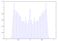
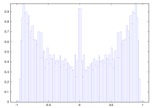
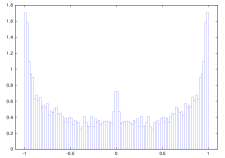
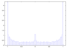
Figure 2. Plots illustrating Corollary 1.7 and the second statement of Theorem 1.10. Each histogram corresponds to the spectrum of a single realization of $K$ with $n=5000$, for various choices of $\mathcal{L}$. From left to right and top to bottom, $\mathcal{L}$ is uniform on $[0,t]$ with $t=1/8$, $t=1/4$, $t=1/2$, and $t=1$.

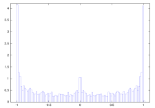
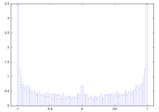
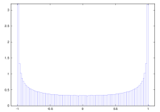
Figure 3. Plots illustrating Corollary 1.7. Each histogram corresponds to the spectrum of a single realization of $K$ with $n=5000$, for various choices of $\mathcal{L}$. From left to right and top to bottom, $\mathcal{L}$ is uniform on $[t,1-t]$ with $t=0$, $t=1/8$, $t=1/4$, $t=1/2$. The last case corresponds to the arc–sine limiting spectral distribution mentioned in Remark 1.8.

which confirms the known fact that $\mu$ is the arc–sine law on $[-1,+1]$ in this case (see e.g. [20, III.4 page 80]). More generally, a very similar computation reveals that if $\mathcal{L}=\delta_{p}$ with $0<p<1$ then $\mathcal{\mu}$ is the arc–sine law on $[-2\sqrt{p(1-p)}\,,\,+2\sqrt{p(1-p)}]$. Figures 1-2-3 display simulations illustrating Corollary 1.7 for various other choices of $\mathcal{L}$.

Remark 1.9 (Non–universality).

The law $\mu$ in Corollary 1.7 is not universal, in the sense that it depends on many “Beta-moments” of $\mathcal{L}$, in contrast with the complete graph case where the limiting spectral distribution depends on $\mathcal{L}$ only via its first two moments.

We now turn to the edge behavior of $\sigma(K)$ where $K$ is as in (10). Since $K$ has period $2$, one has $\lambda_{n}(K)=-1$ and we are interested in the behavior of $\lambda_{2}(K)=-\lambda_{n-1}(K)$ as $n$ goes to infinity. Since the limiting spectral distribution $\mu$ is symmetric, the convex hull of its support is of the form $[-\alpha_{\mu},+\alpha_{\mu}]$ for some $0\leq\alpha_{\mu}\leq 1$. The following result gives information on $\alpha_{\mu}$. The reader may forge many conjectures in the same spirit for the map $\mathcal{L}\mapsto\mu$ from the simulations given by Figures 1-2-3.

Theorem 1.10 (Edge behavior for i.i.d. environment).

Let $K$ be the random birth-and-death Markov kernel (10) where $(V_{i})_{i\geq 2}$ are i.i.d. of law $\mathcal{L}$ on $[0,1]$. Let $\mu$ be the symmetric limiting spectral distribution on $[-1,+1]$ which appears in Corollary 1.7. Let $[-\alpha_{\mu},+\alpha_{\mu}]$ be the convex hull of the support of $\mu$. If $\mathcal{L}$ has a positive density at $1/2$ then $\alpha_{\mu}=1$. Consequently, almost surely,

$$\lambda_{2}(K)=-\lambda_{n-1}(K)=1+o(1).$$

On the other hand, if $\mathcal{L}$ is supported on $[0,t]$ with $0<t<1/2$ or on $[t,1]$ with $1/2<t<1$ then almost surely $\limsup_{n\to\infty}\lambda_{2}(K)<1$ and therefore $\alpha_{\mu}<1$.

The proof of Theorem 1.10 is given in Section 3. The speed of convergence of $\lambda_{2}(K)-1$ to $0$ is highly dependent on the choice of the law $\mathcal{L}$. As an example, if e.g.

$$\mathds{E}\left[\log\frac{V}{1-V}\right]=0\quad\text{and}\quad\mathds{E}\left[\left(\log\frac{V}{1-V}\right)^{2}\right]>0$$

where $V$ has law $\mathcal{L}$, then $K$ is the so called Sinai random walk on $\{1,\ldots,n\}$. In this case, by a slight modification of the analysis of [14], one can prove that almost surely,

$$-\infty<\liminf_{n\to\infty}\frac{1}{\sqrt{n}}\log(1-\lambda_{2}(K))\leq\limsup_{n\to\infty}\frac{1}{\sqrt{n}}\log(1-\lambda_{2}(K))<0.$$

Thus, the convergence to the edge here occurs exponentially fast in $\sqrt{n}$. On the other hand, if for instance $\mathcal{L}=\delta_{1/2}$ (simple reflected random walk on $\{1,\ldots,n\}$) then it is known that $1-\lambda_{2}(K)$ decays as $n^{-2}$ only.

We conclude with a list of remarks and open problems.

Fluctuations at the edge. An interesting problem concerns the fluctuations of $\lambda_{2}(\sqrt{n}K)$ around its limiting value $2\sigma$ in the complete graph model. Under suitable moments conditions on $\mathcal{L}$, one may seek for a deterministic sequence $(a_{n})$, and a probability distribution $\mathcal{D}$ on $\mathds{R}$ such that

(11) $$a_{n}\left(\lambda_{2}(\sqrt{n}K)-2\sigma\right)\overset{\text{d}}{\underset{n\to\infty}{\longrightarrow}}\mathcal{D}$$

where “$\overset{d}{\to}$” stands for convergence in distribution. The same may be asked for the random variable $\lambda_{n}(\sqrt{n}K)+2\sigma$. Computer simulations suggest that $a_{n}\approx n^{2/3}$ and that $\mathcal{D}$ is close to a Tracy-Widom distribution. The heuristics here is that $\lambda_{2}(\sqrt{n}K)$ behaves like the $\lambda_{1}$ of a centered Gaussian random symmetric matrix. The difficulty is that the entries of $K$ are not i.i.d., not centered, and of course not Gaussian.

Symmetric Markov generators. Rather than considering the random walk with infinitesimal generator $K-I$ on the complete graph as we did, one may start with the symmetric infinitesimal generator $G$ defined by $G_{i,j}=G_{j,i}=U_{i,j}$ for every $1\leq i<j\leq n$ and $G_{i,i}=-\sum_{j\neq i}G_{i,j}$ for every $1\leq i\leq n$. Here $(U_{i,j})_{1\leq i<j}$ is a triangular array of i.i.d. real random variables of law $\mathcal{L}$. For this model, the uniform probability measure $\mathcal{U}$ is reversible and invariant. The bulk behavior of such random matrices has been investigated in [16].

Non–reversible Markov ensembles. A non–reversible model is obtained when the underlying complete graph is oriented. That is each vertex $i$ has now (besides the loop) $n-1$ outgoing edges $(i,j)$ and $n-1$ incoming edges $(j,i)$. On each of these edges we place an independent positive weight $V_{i,j}$ with law $\mathcal{L}$, and on each loop an independent positive weight $V_{i,i}$ with law $\mathcal{L}$. This gives us a non–reversible stochastic matrix

$$\widetilde{K}_{i,j}=\frac{V_{i,j}}{\sum_{k=1}^{n}V_{i,k}}\,.$$

The spectrum of $\widetilde{K}$ is now complex. If $\mathcal{L}$ is exponential, then the matrix $\widetilde{K}$ describes the Dirichlet Markov Ensemble considered in [17]. Numerical simulations suggest that if $\mathcal{L}$ has, say, finite positive variance, then the ESD of $n^{1/2}\widetilde{K}$ converges weakly as $n\to\infty$ to the uniform law on the unit disc of the complex plane (circular law). At the time of writing, this conjecture is still open. Note that the ESD of the i.i.d. matrix $(n^{-1/2}V_{i,j})_{1\leq{i,j}\leq n}$ is known to converge weakly to the circular law; see [35] and references therein.

Heavy–tailed weights. Recently, remarkable work has been devoted to the spectral analysis of large dimensional symmetric random matrices with heavy–tailed i.i.d. entries, see e.g. [33, 2, 6, 38, 8]. Similarly, on the complete graph, one may consider the bulk and edge behavior of the random reversible Markov kernels constructed by (1) when the law $\mathcal{L}$ of the weights is heavy–tailed (i.e. with at least an infinite second moment). In that case, and in contrast with Theorem 1.1, the scaling is not $\sqrt{n}$ and the limiting spectral distribution is not Wigner’s semi–circle law. We study such heavy–tailed models elsewhere [12]. Another interesting model is the so called trap model which corresponds to put heavy–tailed weights only on the diagonal of $\mathbf{U}$ (holding times), see e.g. [13] for some recent advances.

2. Proofs for the complete graph model

Here we prove Theorems 1.1, 1.2, Proposition 1.5 and Corollary 1.3. In the whole sequel, we denote by $L^{2}(1)$ the Hilbert space $\mathds{R}^{n}$ equipped with the scalar product

$$\langle x,y\rangle=\sum_{i=1}^{n}x_{i}\,y_{i}.$$

The following simple lemma allows us to work with symmetric matrices when needed.

Lemma 2.1 (Spectral equivalence).

Almost surely, for large enough $n$, the spectrum of the reversible Markov matrix $K$ coincides with the spectrum of the symmetric matrix $S$ defined by

$$S_{i,j}=\sqrt{\frac{\rho_{i}}{\rho_{j}}}K_{i,j}=\frac{U_{i,j}}{\sqrt{\rho_{i}\rho_{j}}}\,.$$

Moreover, the corresponding eigenspaces dimensions also coincide.

Proof.

Almost surely, for large enough $n$, all the $\rho_{i}$ are positive and $K$ is self–adjoint as an operator from $L^{2}(\rho)$ to $L^{2}(\rho)$, where $L^{2}(\rho)$ denotes $\mathds{R}^{n}$ equipped with the scalar product

$$\left<x,y\right>_{\rho}=\sum_{i=1}^{n}\rho_{i}\,x_{i}\,y_{i}.$$

It suffices to observe that a.s. for large enough $n$, the map $x\mapsto\widehat{x}$ defined by

$$\widehat{x}=\left(x_{1}\sqrt{\rho_{1}},\ldots,x_{n}\sqrt{\rho_{n}}\right)$$

is an isometry from $L^{2}(\rho)$ to $L^{2}(1)$ and that for any $x,y\in\mathds{R}^{n}$ and $1\leq i\leq n$, we have

$$(Kx)_{i}=\sum_{j=1}^{n}K_{i,j}x_{j}$$

and

$$\left<Kx,y\right>_{\rho}=\sum_{i,j=1}^{n}K_{i,j}x_{j}y_{i}\rho_{i}=\sum_{i,j=1}^{n}U_{i,j}x_{j}y_{i}=\sum_{i,j=1}^{n}S_{i,j}\widehat{x}_{i}\widehat{y}_{j}=\left<S\widehat{x},\widehat{y}\right>.$$

∎

The random symmetric matrix $S$ has non–centered, non–independent entries. Each entry of $S$ is bounded and belongs to the interval $[0,1]$, since for every $1\leq i,j\leq n$, we have $S_{i,j}\leq U_{i,j}/\sqrt{U_{i,j}U_{j,i}}=1$. In the sequel, for any $n\times n$ real symmetric matrix $A$, we denote by

$$\lambda_{n}(A)\leq\cdots\leq\lambda_{1}(A)$$

its ordered spectrum. We shall also denote by $\|A\|$ the operator norm of $A$, defined by

$$\|A\|^{2}=\max_{x\in\mathds{R}^{n}}\frac{\langle Ax,Ax\rangle}{\langle x,x\rangle}.$$

Clearly, $\|A\|=\max(\lambda_{1}(A),-\lambda_{n}(A))$. To prove Theorem 1.1 we shall compare the symmetric random matrix $\sqrt{n}\,S$ with the symmetric $n\times n$ random matrices

(12) $$W_{i,j}=\frac{U_{i,j}-1}{\sqrt{n}}\quad\text{and}\quad\widetilde{W}_{i,j}=\frac{U_{i,j}}{\sqrt{n}}.$$

Note that $W$ defines a so called Wigner matrix, i.e. $W$ is symmetric and it has centered i.i.d. entries with finite positive variance. We shall also need the non–centered matrix $\widetilde{W}$. It is well known that under the sole assumption $\sigma^{2}\in(0,\infty)$ on $\mathcal{L}$, almost surely,

$$\mu_{W}\underset{n\to\infty}{\overset{w}{\longrightarrow}}\mathcal{W}_{2\sigma}\quad\text{and}\quad\mu_{\widetilde{W}}\underset{n\to\infty}{\overset{w}{\longrightarrow}}\mathcal{W}_{2\sigma}$$

where $\mu_{W}$ and $\mu_{\widetilde{W}}$ are the ESD of $W$ and $\widetilde{W}$, see e.g. [3, Theorems 2.1 and 2.12]. Note that $\widetilde{W}$ is a rank one perturbation of $W$, which implies that the spectra of $W$ and $\widetilde{W}$ are interlaced (Weyl-Poincaré inequalities, see e.g. [24, 3]). Moreover, under the assumption of finite fourth moment on $\mathcal{L}$, it is known that almost surely

$$\lambda_{n}(W)\to-2\sigma\quad\text{and}\quad\lambda_{1}(W)\to+2\sigma.$$

In particular, almost surely,

(13) $$\|W\|=2\sigma+o(1)\,.$$

On the other hand, and still under the finite fourth moment assumption, almost surely,

$$\lambda_{1}(\widetilde{W})\to+\infty\quad\text{while}\quad\lambda_{2}(\widetilde{W})\to+2\sigma\quad\text{and}\quad\lambda_{n}(\widetilde{W})\to-2\sigma$$

see e.g. [4, 21, 3]. Heuristically, when $n$ is large, the law of large numbers implies that $\rho_{i}$ is close to $n$ (recall that here $\mathcal{L}$ has mean $1$), and thus $\sqrt{n}\,S$ is close to $\widetilde{W}$. The main tools needed for a comparison of the matrix $\sqrt{n}S$ with $\widetilde{W}$ are given in the following subsection.

Uniform law of large numbers

We shall need the following Kolmogorov-Marcinkiewicz-Zygmund strong uniform law of large numbers, related to Baum-Katz type theorems.

Lemma 2.2.

Let $(A_{i,j})_{i,j\geq 1}$ be a symmetric array of i.i.d.  random variables. For any reals $a>1/2$, $b\geq 0$, and $M>0$, if $\mathds{E}(|A_{1,1}|^{(1+b)/a})<\infty$ then

$$\max_{1\leq i\leq Mn^{b}}\biggr{|}\sum_{j=1}^{n}(A_{i,j}-c)\biggr{|}=o(n^{a})\quad\text{a.s.}\quad\text{where}\quad c=\begin{cases}\mathds{E}(A_{1,1})&\text{if $a\leq 1$}\\ \text{any number}&\text{if $a>1$}.\end{cases}$$

Proof.

This result is proved in [5, Lemma 2] for a non–symmetric array. The symmetry makes the random variables $(\sum_{j=1}^{n}A_{i,j})_{i\geq 1}$ dependent, but a careful analysis of the argument shows that this is not a problem except for a sort of converse, see [5, Lemma 2] for details. ∎

Lemma 2.3.

If $\mathcal{L}$ has finite moment of order $\kappa\in[1,2]$ then

(14) $$\max_{1\leq i\leq n^{\kappa-1}}\left|\frac{\rho_{i}}{n}-1\right|=o(1)$$

almost surely, and in particular, if $\mathcal{L}$ has finite second moment, then almost surely

(15) $$\max_{1\leq i\leq n}\left|\frac{\rho_{i}}{n}-1\right|=o(1).$$

Moreover if $\mathcal{L}$ has finite moment of order $\kappa$ with $2\leq\kappa<4$, then almost surely

(16) $$\max_{1\leq i\leq n}\left|\frac{\rho_{i}}{n}-1\right|=o(n^{\frac{2-\kappa}{\kappa}}).$$

Additionally, if $\mathcal{L}$ has finite fourth moment, then almost surely

(17) $$\sum_{i=1}^{n}\left(\frac{\rho_{i}}{n}-1\right)^{2}=O(1)\,.$$

Proof.

The result (14) follows from Lemma 2.2 with

$$A_{i,j}=U_{i,j},\quad a=M=1,\quad b=\kappa-1.$$

We recover the standard strong law of large numbers with $\kappa=1$. The result (16) – and therefore (15) setting $\kappa=2$ – follows from Lemma 2.2 with this time

$$A_{i,j}=U_{i,j},\quad a=2/\kappa,\quad b=M=1.$$

Proof of (17). We set $\epsilon_{i}=n^{-1}\rho_{i}-1$ for every $1\leq i\leq n$. Since $\mathcal{L}$ has finite fourth moment, the result (13) for the centered Wigner matrix $W$ defined by (12) gives that

$$\sum_{i=1}^{n}\epsilon_{i}^{2}=\frac{\langle W1,W1\rangle}{\langle 1,1\rangle}\leq\|W\|^{2}=4\sigma^{2}+o(1)=O(1)$$

almost surely. ∎

We are now able to give a proof of Proposition 1.5.

Proof of Proposition 1.5.

Since $\mathcal{L}$ has finite first moment, by the strong law of large numbers,

$$\rho_{1}+\cdots+\rho_{n}=\sum_{i=1}^{n}U_{i,i}+2\!\!\sum_{1\leq i<j\leq n}\!\!U_{i,j}=n^{2}(1+o(1))$$

almost surely. For every fixed $i\geq 1$, we have also $\rho_{i}=n(1+o(1))$ almost surely. As a consequence, for every fixed $i\geq 1$, almost surely,

$$\hat{\rho}_{i}=\frac{\rho_{i}}{\rho_{1}+\cdots+\rho_{n}}=\frac{n(1+o(1))}{n^{2}(1+o(1))}=\frac{1}{n}(1+o(1)).$$

Moreover, since $\mathcal{L}$ has finite second moment, the $o(1)$ in the right hand side above is uniform over $1\leq i\leq n$ thanks to (15) of Lemma 2.3. This achieves the proof. ∎

Note that, under the second moment assumption, $\hat{\rho}_{i}=n^{-1}(1+O(\delta))$ for $1\leq i\leq n$, where

(18) $$\delta:=\max_{1\leq i\leq n}|\epsilon_{i}|=o(1)\,,\quad\text{with}\quad\epsilon_{i}:=n^{-1}\rho_{i}-1.$$

We will repeatedly use the notation (18) in the sequel.

Bulk behavior

Lemma 2.1 reduces Theorem 1.1 to the study of the ESD of $\sqrt{n}S$, a symmetric matrix with non independent entries. One can find in the literature many extensions of Wigner’s theorem to symmetric matrices with non–i.i.d. entries. However, none of these results seems to apply here directly.

Proof of Theorem 1.1.

We first recall a standard fact about comparison of spectral densities of symmetric matrices. Let $L(F,G)$ denote the Lévy distance between two cumulative distribution functions $F$ and $G$ on $\mathds{R}$, defined by

$$L(F,G)=\inf\{\varepsilon>0\text{ such that }F(\cdot-\varepsilon)-\epsilon\leq G\leq F(\cdot+\epsilon)+\epsilon)\}\,.$$

It is well known [7] that the Lévy distance is a metric for weak convergence of probability distributions on $\mathds{R}$. If $F_{A}$ and $F_{B}$ are the cumulative distribution functions of the empirical spectral distributions of two hermitian $n\times n$ matrices $A$ and $B$, we have the following bound for the third power of $L(F_{A},F_{B})$ in terms of the trace of $(A-B)^{2}$:

(19) $$L^{3}(F_{A},F_{B})\leq\frac{1}{n}\mathrm{Tr}((A-B)^{2})=\frac{1}{n}\sum_{i,j=1}^{n}(A_{i,j}-B_{i,j})^{2}\,.$$

The proof of this estimate is a consequence of the Hoffman-Wielandt inequality [23], see also [3, Lemma 2.3]. By Lemma 2.1, we have $\sqrt{n}\lambda_{k}(K)=\lambda_{k}(\sqrt{n}S)$ for every $1\leq k\leq n$. We shall use the bound (19) for the matrices $A=\sqrt{n}S$ and $B=\widetilde{W}$, where $\widetilde{W}$ is defined in (12). We will show that a.s.

(20) $$\frac{1}{n}\sum_{i,j=1}(A_{i,j}-B_{i,j})^{2}=O(\delta^{2})\,,$$

where $\delta=\max_{i}|\epsilon_{i}|$ as in (18). Since $\mathcal{L}$ has finite positive variance, we know that the ESD of $B$ tends weakly as $n\to\infty$ to the semi–circle law on $[-2\sigma,+2\sigma]$. Therefore the bound (20), with (19) and the fact that $\delta\to 0$ as $n\to\infty$ is sufficient to prove the theorem. We turn to a proof of (20). For every $1\leq i,j\leq n$, we have

$$A_{i,j}-B_{i,j}=\frac{U_{i,j}}{\sqrt{n}}\left(\frac{n}{\sqrt{\rho_{i}\rho_{j}}}-1\right)\,.$$

Set, as usual $\rho_{i}=n(1+\epsilon_{i})$ and define $\psi_{i}=(1+\epsilon_{i})^{-\frac{1}{2}}-1$. Note that by Lemma 2.3, almost surely, $\psi_{i}=O(\delta)$ uniformly in $i=1,\dots,n$. Also,

$$\frac{n}{\sqrt{\rho_{i}\rho_{j}}}-1=(1+\psi_{i})(1+\psi_{j})-1=\psi_{i}+\psi_{j}+\psi_{i}\psi_{j}\,.$$

In particular, $\frac{n}{\sqrt{\rho_{i}\rho_{j}}}-1=O(\delta)$. Therefore

$$\frac{1}{n}\sum_{i,j=1}(A_{i,j}-B_{i,j})^{2}\leq O(\delta^{2})\,\left(\frac{1}{n^{2}}\sum_{i,j=1}^{n}U_{i,j}^{2}\right)\,.$$

By the strong law of large numbers, $\frac{1}{n^{2}}\sum_{i,j=1}^{n}U_{i,j}^{2}\to\sigma^{2}+1$ a.s., which implies (20). ∎

Edge behavior

We turn to the proof of Theorem 1.2 which concerns the edge of $\sigma(\sqrt{n}S)$.

Proof of Theorem 1.2.

Thanks to Lemma 2.1 and the global behavior proven in Theorem 1.1, it is enough to show that, almost surely,

$$\limsup_{n\to\infty}\sqrt{n}\max(|\lambda_{2}(S)|,|\lambda_{n}(S)|)\leq 2\sigma\,.$$

Since $K$ is almost surely irreducible for large enough $n$, the eigenspace of $S$ of the eigenvalue $1$ is almost surely of dimension $1$, and is given by $\mathds{R}(\sqrt{\rho_{1}},\ldots,\sqrt{\rho_{n}})$. Let $P$ be the orthogonal projector on $\mathds{R}\sqrt{\rho}$. The matrix $P$ is $n\times n$ symmetric of rank $1$, and for every $1\leq i,j\leq n$,

$$P_{i,j}=\frac{\sqrt{\rho_{i}\rho_{j}}}{\sum_{k=1}^{n}\rho_{k}}.$$

The spectrum of the symmetric matrix $S-P$ is

$$\{\lambda_{n}(S),\ldots,\lambda_{2}(S)\}\cup\{0\}.$$

By subtracting $P$ from $S$ we remove the largest eigenvalue $1$ from the spectrum, without touching the remaining eigenvalues. Let $\mathcal{V}$ be the random set of vectors of unit Euclidean norm which are orthogonal to $\sqrt{\rho}$ for the scalar product $\left<\cdot,\cdot\right>$ of $\mathds{R}^{n}$. We have then

$$\sqrt{n}\max(|\lambda_{2}(S)|,|\lambda_{n}(S)|)=\max_{v\in\mathcal{V}}\left|\left<\sqrt{n}Sv,v\right>\right|=\max_{v\in\mathcal{V}}|\langle\widetilde{A}v,v\rangle|$$

where $\widetilde{A}$ is the $n\times n$ random symmetric matrix defined by

$$\widetilde{A}_{i,j}=\sqrt{n}(S-P)_{i,j}=\sqrt{n}\left(\frac{U_{i,j}}{\sqrt{\rho_{i}\rho_{j}}}-\frac{\sqrt{\rho_{i}\rho_{j}}}{\sum_{k=1}^{n}\rho_{k}}\right).$$

In Lemma 2.4 below we establish that almost surely $\langle v,(\widetilde{A}-W)v\rangle=O(\delta)+O(n^{-1/2})$ uniformly in $v\in\mathcal{V}$, where $W$ is defined in (12) and $\delta$ is given by (18). Thus, using (13),

$$\left|\langle Wv,v\rangle\right|\leq\max(|\lambda_{1}(W)|,|\lambda_{n}(W)|)=2\sigma+o(1)\,,$$

we obtain that almost surely, uniformly in $v\in\mathcal{V}$,

$$|\langle\widetilde{A}v,v\rangle|\leq|\langle Wv,v\rangle|+|\langle(\widetilde{A}-W)v,v\rangle|=2\sigma+o(1)+O(\delta).$$

Thanks to Lemma 2.3 we know that $\delta=o(1)$ and the theorem follows. ∎

Lemma 2.4.

Almost surely, uniformly in $v\in\mathcal{V}$, we have, with $\delta:=\max_{i}|\epsilon_{i}|$,

$$\langle v,(\widetilde{A}-W)v\rangle=O(\delta)+O(n^{-1/2}).$$

Proof.

We start by rewriting the matrix

$$\widetilde{A}_{i,j}=\frac{\sqrt{n}\,U_{i,j}}{\sqrt{\rho_{i}\rho_{j}}}-\frac{\sqrt{n}\sqrt{\rho_{i}\rho_{j}}}{\sum_{k}\rho_{k}}$$

by expanding around the law of large numbers. We set $\rho_{i}=n(1+\epsilon_{i})$ and we define

$$\varphi_{i}=\sqrt{1+\epsilon_{i}}\,-\,1\quad\text{and}\quad\psi_{i}=\frac{1}{\sqrt{1+\epsilon_{i}}}\,-\,1.$$

Observe that $\varphi_{i}$ and $\psi_{i}$ are of order $\epsilon_{i}$ and by Lemma 2.3, cf. (17) we have a.s.

(21) $$\langle\varphi,\varphi\rangle=\sum_{i}\varphi_{i}^{2}=O(1)\quad\text{and}\quad\langle\psi,\psi\rangle=\sum_{i}\psi_{i}^{2}=O(1)\,.$$

We expand

$$\sqrt{\rho_{i}\rho_{j}}=n(1+\epsilon_{i})^{\frac{1}{2}}(1+\epsilon_{j})^{\frac{1}{2}}=n(1+\varphi_{i})(1+\varphi_{j})\,.$$

Similarly, we have

$$\frac{1}{\sqrt{\rho_{i}\rho_{j}}}=n^{-1}(1+\psi_{i})(1+\psi_{j}).$$

Moreover, writing

$$\sum_{k=1}^{n}\rho_{k}=n^{2}\left(1+\frac{1}{n}\sum_{k}\epsilon_{k}\right)$$

and setting $\gamma:=(1+\frac{1}{n}\sum_{k}\epsilon_{k})^{-1}-1$ we see that

$$\left(\sum_{k=1}^{n}\rho_{k}\right)^{-1}=\frac{1}{n^{2}}\,(1+\gamma)\,.$$

Note that $\gamma=O(\delta)$. Using these expansions we obtain

$$\frac{\sqrt{n}\,U_{i,j}}{\sqrt{\rho_{i}\rho_{j}}}=\frac{1}{\sqrt{n}}\,U_{i,j}(1+\psi_{i})(1+\psi_{j})$$

and

$$\frac{\sqrt{n}\sqrt{\rho_{i}\rho_{j}}}{\sum_{k}\rho_{k}}=\frac{1}{\sqrt{n}}\,(1+\varphi_{i})(1+\varphi_{j})(1+\gamma)\,.$$

From these expressions, with the definitions

$$\Phi_{i,j}=\varphi_{i}+\varphi_{j}+\varphi_{i}\varphi_{j}\quad\text{and}\quad\Psi_{i,j}=\psi_{i}+\psi_{j}+\psi_{i}\psi_{j},$$

we obtain

$$\widetilde{A}_{i,j}=W_{i,j}(1+\Psi_{i,j})+\frac{1}{\sqrt{n}}\,\left[\Psi_{i,j}-\Phi_{i,j}(1+\gamma)+\gamma\right].$$

Therefore, we have

$$\langle v,(W-\widetilde{A})v\rangle=-\sum_{i,j}v_{i}W_{i,j}\Psi_{i,j}v_{j}\;+\frac{1+\gamma}{\sqrt{n}}\,\langle v,\Phi v\rangle-\frac{1}{\sqrt{n}}\,\langle v,\Psi v\rangle-\frac{\gamma}{\sqrt{n}}\,\langle v,1\rangle^{2}.$$

Let us first show that

(22) $$\langle v,1\rangle=O(1)\,.$$

Indeed, $v\in\mathcal{V}$ implies that for any $c\in\mathds{R}$,

$$\langle v,1\rangle=\langle v,1-c\sqrt{\rho}\rangle.$$

Taking $c=1/\sqrt{n}$ we see that

$$1-c\sqrt{\rho_{i}}=1-\sqrt{1+\epsilon_{i}}=-\varphi_{i}.$$

Thus, Cauchy–Schwarz’ inequality implies

$$\langle v,1\rangle^{2}\leq\langle v,v\rangle\langle\varphi,\varphi\rangle$$

and (22) follows from (21) above. Next, we show that

(23) $$\langle v,\Phi v\rangle=O(1).$$

Note that

$$\langle v,\Phi v\rangle=2\langle v,1\rangle\langle v,\varphi\rangle+\langle v,\varphi\rangle^{2}.$$

Since $\langle v,\varphi\rangle^{2}\leq\langle v,v\rangle\langle\varphi,\varphi\rangle$ we see that (23) follows from (21) and (22). In the same way we obtain that $\langle v,\Psi v\rangle=O(1)$. So far we have obtained the estimate

(24) $$\langle v,(W-\widetilde{A})v\rangle=-\sum_{i,j}v_{i}W_{i,j}\Psi_{i,j}v_{j}+O(n^{-1/2}).$$

To bound the first term above we observe that

$$\sum_{i,j}v_{i}W_{i,j}\Psi_{i,j}v_{j} =2\sum_{i}\psi_{i}v_{i}(Wv)_{i}+\sum_{i,j}\psi_{i}v_{i}W_{i,j}\psi_{j}v_{j}$$

$$=2\langle\hat{\psi},Wv\rangle+\langle\hat{\psi},W\hat{\psi}\rangle\,,$$

where $\hat{\psi}$ denotes the vector $\hat{\psi}_{i}:=\psi_{i}v_{i}$. Note that

$$\langle\hat{\psi},\hat{\psi}\rangle=\sum_{i}\psi_{i}^{2}v_{i}^{2}\leq O(\delta^{2})\langle v,v\rangle=O(\delta^{2}).$$

Therefore, by definition of the norm $\|W\|$

$$|\langle\hat{\psi},W\hat{\psi}\rangle|\leq\sqrt{\langle\hat{\psi},\hat{\psi}\rangle}\sqrt{\langle W\hat{\psi},W\hat{\psi}\rangle}\leq\|W\|\,\langle\hat{\psi},\hat{\psi}\rangle=O(\delta^{2})\,\|W\|\,.$$

Similarly, we have

$$|\langle\hat{\psi},Wv\rangle|\leq\sqrt{\langle\hat{\psi},\hat{\psi}\rangle}\sqrt{\langle Wv,Wv\rangle}\leq O(\delta)\,\|W\|\sqrt{\langle v,v\rangle}=O(\delta)\,\|W\|\,.$$

From (13), $\|W\|=2\sigma+o(1)=O(1)$. Therefore, going back to (24) we have obtained

$$\langle v,(W-\widetilde{A})v\rangle=O(\delta)+O(n^{-1/2}).$$

∎

We end this section with the proof of Corollary 1.3.

Proof of Corollary 1.3.

By Theorem 1.2, almost surely, and for any compact subset $C$ of $\mathds{R}$ containing strictly $[0,2\sigma]$, the law $\widetilde{\mu}_{\sqrt{n}K}$ is supported in $C$ for large enough $n$. On the other hand, since $\mu_{\sqrt{n}K}=(1-n^{-1})\widetilde{\mu}_{\sqrt{n}K}+n^{-1}\delta_{\sqrt{n}}$, we get from Theorem 1.1 that almost surely, $\widetilde{\mu}_{\sqrt{n}K}$ tends weakly to $\mathcal{W}_{2\sigma}$ as $n\to\infty$. Now, for sequences of probability measures supported in a common compact set, by Weierstrass’ theorem, weak convergence is equivalent to Wasserstein convergence $W_{p}$ for every $p\geq 1$. Consequently, almost surely,

(25) $$\lim_{n\to\infty}W_{p}(\widetilde{\mu}_{\sqrt{n}K},\mathcal{W}_{2\sigma})=0.$$

for every $p\geq 1$. It remains to study $W_{p}(\mu_{\sqrt{n}K},\mathcal{W}_{2\sigma})$. Recall that if $\nu_{1}$ and $\nu_{2}$ are two probability measures on $\mathds{R}$ with cumulative distribution functions $F_{\nu_{1}}$ and $F_{\nu_{2}}$ with respective generalized inverses $F_{\nu_{1}}^{-1}$ and $F_{\nu_{2}}^{-1}$, then, for every real $p\geq 1$, we have, according to e.g. [36, Remark 2.19 (ii)],

(26) $$W_{p}(\nu_{1},\nu_{2})^{p}=\int_{0}^{1}\!\left|F_{\nu_{1}}^{-1}(t)-F_{\nu_{2}}^{-1}(t)\right|^{p}\,dt.$$

Let us take $\nu_{1}=\mu_{\sqrt{n}K}=(1-n^{-1})\widetilde{\mu}_{\sqrt{n}K}+n^{-1}\delta_{\sqrt{n}}$ and $\nu_{2}=\mathcal{W}_{2\sigma}$. Theorem 1.2 gives $\lambda_{2}(\sqrt{n}K)<\infty$ a.s. Also, a.s., for large enough $n$, and for every $t\in(0,1)$,

$$F_{\nu_{1}}^{-1}(t)=F_{\mu_{\sqrt{n}K}}^{-1}(t)=\sqrt{n}\mathds{1}_{[1-n^{-1},1)}(t)+F_{\widetilde{\mu}_{\sqrt{n}K}}^{-1}(t+n^{-1})\mathds{1}_{(0,1-n^{-1})}(t).$$

The desired result follows then by plugging this identity in (26) and by using (25). ∎

3. Proofs for the chain graph model

In this section we prove the bulk results in Theorem 1.6 and Corollary 1.7 and the edge results in Theorem 1.10.

Bulk behavior

Proof of Theorem 1.6.

Since $\mu_{K}$ is supported in the compact set $[-1,+1]$ which does not depend on $n$, Weierstrass’ theorem implies that the weak convergence of $\mu_{K}$ as $n\to\infty$ is equivalent to the convergence of all moments, and is also equivalent to the convergence in Wasserstein distance $W_{p}$ for every $p\geq 1$. Thus, it suffices to show that a.s. for any $\ell\geq 0$, the $\ell^{\text{th}}$ moment of $\mu_{K}$ converges to $\mathds{E}[r_{\ell}^{\mathbf{p}}(0)]$ as $n\to\infty$. The sequence $(\mathds{E}[r^{\mathbf{p}}_{\ell}(0)])_{\ell\geq 0}$ will be then necessarily the sequence of moments of a probability measure $\mu$ on $[-1,+1]$ which is the unique adherence value of $\mu_{K}$ as $n\to\infty$.

For any $\ell\geq 0$ and $i\geq 1$ let $r_{\ell}^{\mathbf{p},n}(i)$ be the probability of return to $i$ after $\ell$ steps for the random walk on $\{1,\ldots,n\}$ with kernel $K$. Clearly, $r_{\ell}^{\mathbf{p},n}(i)=r_{\ell}^{\mathbf{p}}(i)$ whenever $1+\ell<i<n-\ell$. Therefore, for every fixed $\ell$, the ergodic theorem implies that almost surely,

$$\lim_{n\to\infty}\frac{1}{n}\sum_{i=1}^{n}r_{\ell}^{\mathbf{p},n}(i)=\lim_{n\to\infty}\frac{1}{n}\sum_{i=1}^{n}r_{\ell}^{\mathbf{p}}(i)=\mathds{E}[r_{\ell}^{\mathbf{p}(0)}].$$

This ends the proof. ∎

Proof of Corollary 1.7.

The desired convergence follows immediately from Theorem 1.6 with $\mathbf{p}(i)=(1-V_{i},0,V_{i})$ for every $i\geq 1$. The expression of the moments of $\mu$ follows from a straightforward path–counting argument for the return probabilities of a one-dimensional random walk. ∎

Let us mention that the proof of Corollary 1.7 could have been obtained via the trace-moment method for symmetric tridiagonal matrices. Indeed, an analog of Lemma 2.1 allows one to replace $K$ by a symmetric tridiagonal matrix $S$. Although the entries of $S$ are not independent, the desired result follows from a variant of the proof used by Popescu for symmetric tridiagonal matrices with independent entries [30, Theorem 2.8]. We omit the details.

Remark 3.1 (Computation of the moments of $\mu$ for Beta environments).

As noticed in Remark 1.8, the limiting spectral distribution $\mu$ is the arc–sine law when $\mathcal{L}=\delta_{1/2}$. Assume now that $\mathcal{L}$ is uniform on $[0,1]$. Then for every integers $m\geq 0$ and $n\geq 0$,

$$\mathds{E}(V^{m}(1-V)^{n})=\int_{0}^{1}\!u^{m}(1-u)^{n}\,du=\mathrm{Beta}(n+1,m+1)= \frac{\Gamma(n+1)\Gamma(m+1)}{\Gamma(n+m+2)}$$

which gives

$$\mathds{E}(V^{m}(1-V)^{n})=\frac{n!m!}{(n+m+1)!}=\frac{1}{(n+m+1)\binom{n+m}{m}}.$$

The law of $\binom{n+m}{m}V^{m}(1-V)^{n}$ is the law of the probability of having $m$ success in $n+m$ tosses of a coin with a probability of success $p$ uniformly distributed in $[0,1]$. Similar formulas may be obtained when $\mathcal{L}$ is a Beta law $\mathrm{Beta}(\alpha,\beta)$.

Edge behavior

Proof of Theorem 1.10.

Proof of the first statement. It is enough to show that for every $0<a<1$, there exists an integer $k_{a}$ such that for all $k\geq k_{a}$,

(27) $$\int_{-1}^{+1}\!x^{2k}\mu(dx)\geq a^{2k}.$$

By assumption, there exists $C>0$ and $0<t_{0}<1/2$ such that for all $0<t<t_{0}$,

$$\mathds{P}(V\in[1/2-t,1/2+t])\geq Ct$$

where $V$ is random variable of law $\mathcal{L}$. In particular, for all $0<t<t_{0}$,

$$\mathds{E}\left[V^{N_{\gamma}(i)}(1-V)^{N_{\gamma}(i-1)}\right]\geq Ct\left(\frac{1}{2}-t\right)^{N_{\gamma}(i)+N_{\gamma}(i-1)},$$

and, if

$$\|\gamma\|_{\infty}=\max\{i\geq 0:\max(N_{\gamma}(i),N_{\gamma}(-i))\geq 1\}$$

then

$$\int_{-1}^{+1}\!x^{2k}\mu(dx) \geq\sum_{\gamma\in D_{k}}\prod_{i\in\mathds{Z}}Ct\left(\frac{1}{2}-t\right)^{N_{\gamma}(i)+N_{\gamma}(i-1)}$$

$$\geq\sum_{\gamma\in D_{k}}(Ct)^{2\|\gamma\|_{\infty}}\left(\frac{1}{2}-t\right)^{\sum_{i}N_{\gamma}(i)+N_{\gamma}(i-1)}$$

$$\geq\left(\frac{1}{2}-t\right)^{2k}\sum_{\gamma\in D_{k}}(Ct)^{2\|\gamma\|_{\infty}}$$

$$\geq\left(\frac{1}{2}-t\right)^{2k}|D_{k,\alpha}|(Ct)^{2k^{\alpha}},$$

where $D_{k,\alpha}=\{\gamma\in D_{k}:\|\gamma\|_{\infty}\leq k^{\alpha}\}$. Now, from the Brownian Bridge version of Donsker’s Theorem (see e.g. [26] and references therein), for all $\alpha>1/2$,

$$\lim_{k\to\infty}\frac{|D_{k,\alpha}|}{|D_{k}|}=1.$$

Since $|D_{k}|=\mathrm{Card}(D_{k})=\binom{2k}{k}$, Stirling’s formula gives $|D_{k}|\sim 4^{k}(\pi k)^{-1/2}$, and thus

$$\int_{-1}^{+1}\!x^{2k}\mu(dx)\geq(\pi k)^{-1/2}(1-2t)^{2k}(Ct)^{2k^{\alpha}}(1+o(1)).$$

We then deduce the desired result (27) by taking $t$ small enough such that $1-2t>a$ and $1/2<\alpha<1$. This achieves the proof of the first statement.

Proof of the second statement. One can observe that if $\mathcal{L}=\delta_{p}$ for some $p\in(0,1)$ with $p\neq 1/2$, an explicit computation of the spectrum will provide the desired result, in accordance with Remark 1.8. For the general case, we get from [28], for any $2\leq k\leq n-1$,

$$1-\lambda_{2}(K)\geq\frac{1}{4\max(B_{k}^{+},B_{k}^{-})}$$

where

$$B_{k}^{+}=\max_{i>k}\left[\left(\sum_{j=k+1}^{i}\frac{1}{\rho_{j}(1-V_{j})}\right)\sum_{j\geq i}\rho_{j}\right]\quad\text{and}\quad B_{k}^{-}=\max_{i<k}\left[\left(\sum_{j=i}^{k-1}\frac{1}{\rho_{j}V_{j}}\right)\sum_{j\leq i}\rho_{j}\right]$$

with the convention $V_{1}=1-V_{n}=1$. Here we have fixed the value of $n$ and $\rho$ is any invariant (reversible) measure for $K$. It is convenient to take $\rho_{1}=1$ and for every $2\leq i\leq n$

$$\rho_{i}=\frac{V_{2}\cdots V_{i-1}}{(1-V_{2})\cdots(1-V_{i})}.$$

By symmetry, it suffices to consider the case where $\mathcal{L}$ is supported in $[0,t]$ with $0<t<1/2$. Let us take $k=2$. In this case, $B_{2}^{-}=1$, and the desired result will follow if we show that $B_{2}^{+}$ is bounded above by a constant independent of $n$. To this end, we remark first that for any $\ell>j$ we have $\rho_{\ell}=\rho_{j}\prod_{m=j}^{\ell-1}(V_{m}/(1-V_{m+1}))$. Therefore, setting $e^{-\gamma}=t/(1-t)<1$, we have $\rho_{\ell}\leq\rho_{j}e^{-\gamma(\ell-j)}$. It follows that, for any $k<i$,

$$\sum_{j=k+1}^{i}\sum_{\ell\geq i}\frac{\rho_{\ell}}{\rho_{j}(1-V_{j})} \leq\frac{1}{1-t}\sum_{j=k+1}^{i}e^{-\gamma(i-j)}\sum_{\ell\geq i}e^{-\gamma(\ell-i)}$$

$$\leq\frac{(1-e^{-\gamma})^{-2}}{1-t}=\frac{1-t}{(1-2t)^{2}}.$$

In particular, $B_{2}^{+}\leq(1-t)/(1-2t)^{2}$, which concludes the proof. ∎

Acknowledgements. The second author would like to thank the Équipe de Probabilités et Statistique de l’Institut de Mathématiques de Toulouse for kind hospitality. The last author would like to thank Delphine Féral and Sandrine Péché for interesting discussions on the extremal eigenvalues of symmetric non–central random matrices with i.i.d entries.

References

- [1] G. W. Anderson, A. Guionnet, and O. Zeitouni, An Introduction to Random Matrices, Cambridge University Press, 2009, to appear.
- [2] A. Auffinger, G. Ben Arous, and S. Péché, Poisson convergence for the largest eigenvalues of heavy tailed random matrices, Ann. Inst. Henri Poincaré Probab. Stat. 45 (2009), no. 3, 589–610. MR MR2548495
- [3] Z. D. Bai, Methodologies in spectral analysis of large-dimensional random matrices, a review, Statist. Sinica 9 (1999), no. 3, 611–677, With comments by G. J. Rodgers and J. W. Silverstein; and a rejoinder by the author.
- [4] Z. D. Bai and Y. Q. Yin, Necessary and sufficient conditions for almost sure convergence of the largest eigenvalue of a Wigner matrix, Ann. Probab. 16 (1988), no. 4, 1729–1741.
- [5] by same author, Limit of the smallest eigenvalue of a large-dimensional sample covariance matrix, Ann. Probab. 21 (1993), no. 3, 1275–1294.
- [6] G. Ben Arous and A. Guionnet, The spectrum of heavy tailed random matrices, Comm. Math. Phys. 278 (2008), no. 3, 715–751.
- [7] P. Billingsley, Convergence of probability measures, second ed., Wiley Series in Probability and Statistics: Probability and Statistics, John Wiley & Sons Inc., New York, 1999, A Wiley-Interscience Publication.
- [8] G. Biroli, J.-P. Bouchaud, and M. Potters, On the top eigenvalue of heavy-tailed random matrices, Europhys. Lett. EPL 78 (2007), no. 1, Art. 10001, 5.
- [9] D. Boivin and J. Depauw, Spectral homogenization of reversible random walks on in a random environment, Stochastic Process. Appl. 104 (2003), no. 1, 29–56.
- [10] B. Bollobás, Random graphs, second ed., Cambridge Studies in Advanced Mathematics, vol. 73, Cambridge University Press, Cambridge, 2001.
- [11] E. Bolthausen and A.-S. Sznitman, Ten lectures on random media, DMV Seminar, vol. 32, Birkhäuser Verlag, Basel, 2002. MR MR1890289 (2003f:60183)
- [12] Ch. Bordenave, P. Caputo, and D. Chafaï, Spectrum of large random reversible Markov chains – Heavy–tailed weigths on the complete graph, arXiv:0903.3528, 2009.
- [13] A. Bovier and A. Faggionato, Spectral characterization of aging: the REM-like trap model, Ann. Appl. Probab. 15 (2005), no. 3, 1997–2037.
- [14] by same author, Spectral analysis of Sinai’s walk for small eigenvalues, Ann. Probab. 36 (2008), no. 1, 198–254.
- [15] S. Boyd, P. Diaconis, P. Parrilo, and L. Xiao, Symmetry analysis of reversible Markov chains, Internet Math. 2 (2005), no. 1, 31–71.
- [16] W. Bryc, A. Dembo, and T. Jiang, Spectral measure of large random Hankel, Markov and Toeplitz matrices, Ann. Probab. 34 (2006), no. 1, 1–38.
- [17] D. Chafaï, The Dirichlet Markov Ensemble, Journal of Multivariate Analysis 101 (2010), 555–567.
- [18] D. Cheliotis and B. Virag, The spectrum of the random environment and localization of noise, preprint, arXiv.math:0804.4814, to appear in Probability Theory and Related Fields, 2008.
- [19] P. G. Doyle and J. L. Snell, Random walks and electric networks, Carus Mathematical Monographs, vol. 22, Mathematical Association of America, Washington, DC, 1984.
- [20] W. Feller, An introduction to probability theory and its applications. Vol. I, Third edition, John Wiley & Sons Inc., New York, 1968. MR MR0228020 (37 #3604)
- [21] Z. Füredi and J. Komlós, The eigenvalues of random symmetric matrices, Combinatorica 1 (1981), no. 3, 233–241.
- [22] F. Hiai and D. Petz, The semicircle law, free random variables and entropy, Mathematical Surveys and Monographs, vol. 77, American Mathematical Society, Providence, RI, 2000. MR MR1746976 (2001j:46099)
- [23] A. J. Hoffman and H. W. Wielandt, The variation of the spectrum of a normal matrix, Duke Math. J. 20 (1953), 37–39.
- [24] R. Horn and C. Johnson, Topics in matrix analysis, Cambridge University Press, Cambridge, 1991.
- [25] D.A. Levin, Y. Peres, and E.L. Wilmer, Markov chains and mixing times, American Mathematical Society, Providence, RI, 2009, With a chapter by James G. Propp and David B. Wilson. MR MR2466937
- [26] J.-F. Marckert, One more approach to the convergence of the empirical process to the Brownian bridge, Electron. J. Stat. 2 (2008), 118–126. MR MR2386089 (2009a:62230)
- [27] M. L. Mehta, Random matrices, third ed., Pure and Applied Mathematics (Amsterdam), vol. 142, Elsevier/Academic Press, Amsterdam, 2004. MR MR2129906 (2006b:82001)
- [28] L. Miclo, An example of application of discrete Hardy’s inequalities, Markov Process. Related Fields 5 (1999), no. 3, 319–330. MR MR1710983 (2000h:60081)
- [29] R. Montenegro and P. Tetali, Mathematical Aspects of Mixing Times in Markov Chains, Foundations and Trends in Theoretical Computer Science, vol. 1:3, Now Publishers, 2006.
- [30] I. Popescu, General tridiagonal random matrix models, limiting distributions and fluctuations, Probab. Theory Related Fields 144 (2009), no. 1-2, 179–220. MR MR2480789
- [31] L. Saloff-Coste, Lectures on finite Markov chains, Lectures on probability theory and statistics (Saint-Flour, 1996), Lecture Notes in Math., vol. 1665, Springer, Berlin, 1997, pp. 301–413.
- [32] E. Seneta, Non-negative matrices and Markov chains, Springer Series in Statistics, Springer, New York, 2006, Revised reprint of the second (1981) edition [Springer-Verlag, New York; MR0719544]. MR MR2209438
- [33] A. Soshnikov, Poisson statistics for the largest eigenvalues of Wigner random matrices with heavy tails, Electron. Comm. Probab. 9 (2004), 82–91 (electronic).
- [34] A.-S. Sznitman, Topics in random walks in random environment, School and Conference on Probability Theory, ICTP Lect. Notes, XVII, Abdus Salam Int. Cent. Theoret. Phys., Trieste, 2004, pp. 203–266 (electronic). MR MR2198849 (2007b:60247)
- [35] T. Tao and V. Vu, Random matrices: Universality of ESDs and the circular law, preprint arXiv:0807.4898 [math.PR] to appear in the Annals of Probability, 2008.
- [36] C. Villani, Topics in optimal transportation, Graduate Studies in Mathematics, vol. 58, American Mathematical Society, Providence, RI, 2003. MR MR1964483 (2004e:90003)
- [37] Van Vu, Random discrete matrices, Horizons of combinatorics, Bolyai Soc. Math. Stud., vol. 17, Springer, Berlin, 2008, pp. 257–280. MR MR2432537 (2009i:15034)
- [38] I. Zakharevich, A generalization of Wigner’s law, Comm. Math. Phys. 268 (2006), no. 2, 403–414.
- [39] O. Zeitouni, Random walks in random environment, Lectures on probability theory and statistics, Lecture Notes in Math., vol. 1837, Springer, Berlin, 2004, pp. 189–312. MR MR2071631 (2006a:60201)