Time–resolved spectral correlations of long–duration GRBs

Abstract

For a sample of long Gamma–Ray Bursts (GRBs) with known redshift, we study the distribution of the evolutionary tracks on the rest–frame luminosity–peak energy $L_{\rm iso}$–$E_{\rm p}^{\prime}$ diagram. We are interested in exploring the extension of the ‘Yonetoku’ correlation to any phase of the prompt light curve, and in verifying how the high–signal prompt duration time, $T_{f}^{\prime}$  in the rest frame correlates with the residuals of such correlation (Firmani et al. 2006). For our purpose, we analyse separately two samples of time–resolved spectra corresponding to 32 GRBs with peak fluxes $\mbox{$F_{\rm p}$}>1.8$ phot cm^-2 s^-1  from the Swift–BAT detector, and 7 bright GRBs from the CGRO–BATSE detector previously processed by Kaneko et al. (2006). After constructing the $L_{\rm iso}$–$E_{\rm p}^{\prime}$ diagram, we discuss the relevance of selection effects, finding that they could affect significantly the correlation. However, we find that these effects are much less significant in the $L_{\rm iso}$$T_{f}^{\prime}$–$E_{\rm p}^{\prime}$ diagram, where the intrinsic scatter reduces significantly. We apply further corrections in order to reduce the intrinsic scatter even more. For the sub–samples of GRBs (7 from Swift and 5 from CGRO) with measured jet break time, $t_{\rm j}$, we analyse the effects of correcting $L_{\rm iso}$ by jet collimation. We find that (i) the scatter around the correlation is reduced, and (ii) this scatter is dominated by the internal scatter of the individual evolutionary tracks. These results suggest that the time integrated ‘Amati’ and ‘Ghirlanda’ correlations are consequences of the time resolved features, not of selection effects, and therefore call for a physical origin. We finally remark the relevance of looking inside the nature of the evolutionary tracks.

1 Introduction

The phenomenological study of long Gamma–Ray Bursts (GRBs), on one hand, brings the possibility to use these extreme cosmic events as tracers of many astronomical and cosmological processes, and on the other, leads to a comprehensive description of the underlying GRB physics (see for recent reviews Mészáros 2006; Ghirlanda, Ghisellini & Firmani 2006; Zhang 2007). The finding of correlations among spectral and energetic properties of the prompt emission has been the main avenue of progress in these directions.

Amati et al. (2002) discovered a correlation between the isotropic–equivalent energy radiated during the whole prompt phase, $E_{\rm iso}$, and the peak energy of the rest–frame time–integrated $\nu f_{\nu}$ spectrum, $<E_{\rm p}^{\prime}>$. The scatter around the $E_{\rm iso}$–$<E_{\rm p}^{\prime}>$ correlation suggests the existence of some hidden parameter(s). Ghirlanda, Ghisellini & Lazzati (2004) have identified such parameter with the jet collimation angle, $\theta_{j}$, and Liang & Zhang (2005) with the rest–frame break–time in the afterglow light curve, $t_{\rm j}$; $\theta_{j}$ is tightly associated to $t_{\rm j}$. Both parameters are time integrated quantities of the outflow in the fireball model. A correlation analogous to the ‘Amati’ one but for the peak isotropic–equivalent luminosity, $L_{\rm iso,p}$, has been first reported by Yonetoku et al. (2004). Later on, for a sample of 19 GRBs, Firmani et al. (2006) have found a strong correlation among $L_{\rm iso,p}$, $<E_{\rm p}^{\prime}>$  and a rest–frame prompt emission high–signal GRB time duration, $T_{f}^{\prime}$. Rossi et al. (2008) have also found a correlation among $L_{\rm iso,p}$, $<E_{\rm p}^{\prime}>$, and $T_{f}^{\prime}$, but with different slopes and scatter. More recently, Collazzi & Schaefer (2008) confirmed the ’Firmani’ correlation, though the scatter they obtained for a larger sample is higher than in Firmani et al. (2006). The homogeneity and the quality of the data seems to be crucial for obtaining reliable statistical results; in this sense, the publicly available large database from the Swift  is by now an invaluable source of data.

The GRB light curves are composed by a sequential superposition of many pulses, possibly originated by individual shock episodes. The spectral and temporal characteristics of these pulses are key ingredients for understanding the prompt emission mechanisms of GRBs (e.g., Ryde & Petrosian 2002). Although there is not a simple pattern to describe the great variety of the light curve morphologies, some relations have been found in GRBs with light curves characterized by a single pulse or a few well–separated pulses. For example, Borgonovo & Ryde (2001) have found a correlation between the (bolometric or spectral peak) energy flux, $F$, and observed $E_{\rm p}$ during the decaying phase of individual, well–defined pulses: $\mbox{$F$}\propto\mbox{$E_{\rm p}$}^{\gamma}$, with a mean $\gamma\approx 2$. Notice that $E_{\rm p}$ in this case is inferred from each time–resolved spectrum. Further, Liang, Dai & Xu (2004) have tested whether or not the relation $\mbox{$F$}\propto\mbox{$E_{\rm p}$}^{2}$ within a burst holds in a sub–sample of 2408 time–resolved spectra for 91 bright CGRO-BATSE GRBs presented by Preece et al. (2000; all kind of pulses are included in this sample). They reported that for 75% of the bursts, the Spearman correlation coefficient is larger than 0.5. Nevertheless, even for the Borgonovo & Ryde sample of well–defined pulses, this correlation has a considerable scatter, which is probably produced by the superpositions of pulses.

If the individual pulses within a burst follow on average the correlation $\mbox{$F$}\propto\mbox{$E_{\rm p}$}^{2}$, then a natural question is whether there exists or not a universal relationship among all GRBs in the rest frame.

Both the ‘Yonetoku’ and the $L_{\rm iso,p}$–$<E_{\rm p}^{\prime}>$–$T_{f}^{\prime}$ correlations (Firmani et al. 2006) were established for GRBs with known $z$ taken from heterogeneous samples, with incomplete available data, and by using hybrid quantities: the flux used to calculate $L_{\rm iso,p}$ is at the peak of the light curve, while both $<E_{\rm p}^{\prime}>$ and the bolometric correction had to be inferred from the time–integrated spectrum. The primary data publicly available from the Swift satellite (Gehrels et al. 2004) offers now the possibility to study the mentioned correlations in the rest–frame and with temporal resolution. Unfortunately, the narrow spectral range of the Swift BAT detector limits and makes difficult the spectral analysis.

By means of time–resolved spectral analysis for a sample of 32 Swift and 7 bright CGRO long GRBs, we will show here that, when multiplying $L_{\rm iso}$ by $T_{f}^{\prime}$, the evolutionary tracks of different GRBs form a well defined correlations, with a small scatter. In §2 we develop a heuristic framework to introduce such a connection. The GRB samples used and the spectral analysis are presented in §3. The construction of correlations with the prompt time–resolved data, the analysis of the selection effects, and a discussion of the results are presented in §4.1. In §4.2, we present our attempt to further reduce the scatter around the correlations by introducing the jet collimation correction. We show that most of the remaining scatter in the overall correlations is due to the individual scatter of each evolutionary track. In §5 we present our conclusions.

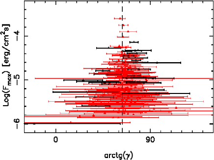
Figure 1: Maximum bolometric flux of a given event versus $\arctan(\gamma)$ for 208 CGRO GRBs with 5 or more time–resolved spectra (from the Kaneko et al. 2006 sample). The quantity $\gamma$ is the slope of the best linear fit to the $F$–$E_{\rm p}^{\prime}$ evolutionary tracks. The $\arctan$ function is used in order the error bars ($3\sigma$) looked symmetric. The vertical dashed line indicates $\arctan 2=63.4$ degrees. Thin red error bars show the events with $\gamma=2$ within $3\sigma$, while thick black error bars indicate the few events incompatible with $\gamma=2$ at the $3\sigma$ level. There is not any systematical trend of $F_{\rm max}$ with $\gamma$, however, the uncertainty and the spread of $\gamma$ around 2 increases as $F_{\rm max}$ decreases.

2 Motivations

Our purpose in this paper is to study, in the rest frame, evolutionary features of the prompt $\gamma-$ray spectra and their connection with other GRB properties. Before discussing the data, we develop an heuristic reasoning aimed to show a potential connection between the phenomenological time–integrated and time–resolved correlations mentioned in the Introduction.

We start from the fact that the prompt evolution of a given burst can be characterised, at least above some flux and/or some peak energy limit, by the dependence $\mbox{$F$}\propto\mbox{$E_{\rm p}$}^{\gamma}$, where $F$ and $E_{\rm p}$ are defined at any given time. The power index $\gamma$ as well as the scatter of the evolutionary correlation could change from burst to burst. Previous analysis showed that the mean value of $\gamma$ is around 2 with some dispersion (Borgonovo & Ryde 2001; Liang et al. 2004). In the rest frame, the burst evolutionary track $\mbox{$F$}\propto\mbox{$E_{\rm p}$}^{\gamma}$ is equivalent to the correlation

$$\mbox{$L_{\rm iso}$}=K\mbox{$E_{\rm p}^{\prime}$}^{\gamma}.$$ (1)

In the logarithmic plane $E_{\rm p}^{\prime}$–$L_{\rm iso}$ the evolutionary track described by Eq. (1) identifies a straight strip with a slope $\gamma$, a zero point, and a specific sector on the strip.

Let us first assume $\gamma=2$. Note that $K$ in this case is independent of the Doppler–boosting factor $D=1/[\Gamma(1-\beta\mu)]$, where $\Gamma$, $\beta c$, and $\mu$ are the Lorentz factor, the velocity, and the cosine of the viewing angle, respectively. By integrating in time, the evolutionary track reduces to

$$\mbox{$E_{\rm iso}$}=KT^{\prime}<\mbox{$E_{\rm p}^{\prime}$}^{2}>,$$ (2)

where $T^{\prime}$ is a rest–frame time scale of the energy emission. Now, if observations give a correlation between $E_{\rm iso}$ and $\mbox{$<E_{\rm p}^{\prime}>$}^{2}$ among different GRBs, (the ‘Amati’ relation), then $KT^{\prime}=k$ becomes approximately a constant independent of each GRB. The conclusion is that scaling $K\propto T^{\prime-1}$, the scatter of the correlation given by Eq. (1) for a sample of GRBs is less than the scatter around the $L_{\rm iso}$–$<E_{\rm p}^{\prime}>$ correlation for the same sample. The fact that $\gamma=2$ for all the GRBs simplifies the previous reasoning: since the evolutionary track given by Eq. (1) and the ‘Amati’ relation show the same slope, then only the zero point of the strip is involved in the scatter around the ‘Amati’ relation. The parallel strips superimpose and thus reduce their occupation region on the plane.

If $\gamma\neq 2$, the situation becomes more intriguing. Now the evolutionary tracks are not aligned with the ‘Amati’ relation and so it is more difficult for them to reduce their occupation region on the $E_{\rm p}^{\prime}$–$L_{\rm iso}$ diagram. Nevertheless, if not only the zero points of the strips, but even the occupation sectors of the evolutionary tracks within the strips conspire in order to agree with the ‘Amati’ relation, then a reduction of their occupation region on the plane (reduction of the scatter) may be reached. This inference allows to hope that $T^{\prime}$ plays a role of a hidden parameter related to the scatter of the correlation Eq. (1).

This heuristic reasoning has actually inspired the present work. Definitively, it is of great interest to verify with high quality prompt time–resolved data whether or not the ‘Firmani’–like time–resolved relation $E_{\rm p}^{\prime}$ vs $\mbox{$L_{\rm iso}$}T^{\prime}$ is obeyed, and to study the scatter around it. If this relation is obeyed, then a corollary is that it establishes a link between the ‘Amati’ $\mbox{$E_{\rm iso}$}-\mbox{$<E_{\rm p}^{\prime}>$}$ and the ‘Yonetoku’ $\mbox{$L_{\rm iso,p}$}-\mbox{$<E_{\rm p}^{\prime}>$}$ relations and, even more importantly, a robust physical ingredient has to exist behind such relation in the sense that at each instant of the prompt the GRB is aware of the duration of the entire process.

Before presenting results from our spectral analysis on Swift and CGRO GRBs with known redshift, we explore the large set of time–resolved spectra from the CGRO data analysed by Kaneko et al. (2006). Since for the great majority of the bursts in this sample the redshift is unknown, we are able to infer only the values of the slope $\gamma$ of the individual correlations $F\propto\mbox{$E_{\rm p}$}^{\gamma}$. The slope should remain the same for the corresponding individual rest–frame correlations $L_{\rm iso}$ vs $E_{\rm p}^{\prime}$.

The Kaneko et al. (2006) sample contains 350 bright GRBs and 7427 time–resolved spectra. Each time–resolved spectrum was fitted to a Band (Band et al. 1993) function. We consider only time–resolved spectra with Band model parameters $\alpha>-2$; $\beta<-2$ and 50$<$$E_{\rm p}$$<$1800 keV (note that $E_{\rm p}$ is in the observer frame) with an uncertainty better than 50% and a time step shorter than 4 s. We assume a bolometric correction given by the Band energy distribution. Finally, we take into account only GRBs with at least 5 time–resolved spectra. Such conditions reduce the sample to 208 GRBs.

Figure 2: $E_{\rm p}^{\prime}$ vs $L_{\rm iso}$ for the time–resolved spectra corresponding to 32 Swift GRBs ($68\%$ CL ellipses) and 7 bright CGRO GRBs ($1\sigma$ error bars). The solid lines connect the data–points of each individual GRB (evolutionary tracks); red colour is for the Swift data and green colour for the CGRO data. The best linear fit to the Swift data is shown with the solid right line, while the $\pm 1\sigma$ intrinsic scatter is indicated with the parallel dot–dashed lines. The upper solid curve corresponds to a limiting observed ($z=0$) flux of $10^{-8}$erg cm^-2 s^-1 and $\mbox{$E_{\rm p}$}\simeq 100$ keV. The ticks along the curve indicate different $z^{\prime}$s: 1, 2,…,9, from left to right.

For this sample, only 16% of the GRB tracks show a disagreement with $\gamma=2$, while the other 84% are compatibles with $\gamma=2$ at the $3\sigma$ level. A similar result, but for less events than here, has been reported by Liang et al. (2004; see their figure 2 for the $F-\mbox{$E_{\rm p}$}$ tracks corresponding to some bursts). We plot in Fig. 1 the maximum bolometric flux, $F_{\rm max}$, of a given event versus $\arctan(\gamma)$; $\arctan$ is used in order the error bars (at 3$\sigma$) looked symmetric. It is clearly seen that only a small fraction of the events (thick black error bars) have values of $\gamma$ different from 2 within $3\sigma$ (vertical dashed line shows $\arctan 2=63.4$ degrees); the majority of them (thin red error bars) show $\gamma$ compatible with 2 within the $3\sigma$ level. In Fig. 1 it is also seen that the correlation slope $\gamma$ is not biased systematically by $F_{\rm max}$, though its uncertainty and the spread around 2 increse as $F_{\rm max}$ decreases. The result shown above opens the question of identifying the physical mechanisms that determine the value of $\gamma$ as well as the intrinsic scatter of each evolutionary track. The fact that a large fraction of GRBs shows $\gamma\simeq 2$, $(i)$ supports the consistency of our research concerning a universal correlation, $(ii)$ provides a natural GRB identification criterion to eventually optimise such correlation, and $(iii)$ allows to study the behaviour of those GRBs with $\gamma\neq 2$.

name	z	$T_{f}$	$t_{\rm j}$	$\rm{Lg}<\mbox{$E_{\rm p}$}^{\prime}>$	$\rm{Lg}\mbox{$E_{\rm iso}$}$	N
		(sec)	(days)	(keV)	($10^{50}$ erg)
050315	1.949	15.00[0.50]				1
050318	1.440	4.00[0.10]		2.45[0.04]	2.07[0.11]	2
050401	2.900	6.20[0.10]	1.50[0.50]	3.45[0.23]	3.51[0.14]	3
050505	4.270	11.80[0.10]		3.54[0.16]	3.13[0.12]	2
050525	0.606	3.10[0.02]	0.30[0.10]	2.33[0.01]	2.34[0.01]	19
050603	2.821	2.10[0.10]		3.68[0.30]	3.55[0.22]	3
050820A	2.612	12.00[0.40]	15.00[8.00]	3.12[0.09]	3.99[0.03]	2
050922C	2.198	1.44[0.02]		3.36[0.22]	2.63[0.14]	6
051109	2.346	6.90[0.20]		2.97[0.16]	2.80[0.19]	1
051111	1.549	11.60[0.10]		3.36[0.34]	2.80[0.22]	1
060206	4.048	2.70[0.10]		3.29[0.06]	2.59[0.06]	5
060210	3.910	35.00[3.00]	2.20[0.90]	3.45[0.14]	3.52[0.10]	4
060418	1.490	16.20[0.30]				3
060526	3.221	12.30[0.30]	2.80[0.30]	2.02[0.09]	2.41[0.05]	1
060614	0.125	28.70[0.10]	1.38[0.04]	1.74[0.36]	1.40[0.17]	6
060904B	0.703	10.00[0.30]		2.36[0.13]	1.44[0.13]	5
060906	3.685	11.50[0.20]		2.99[0.09]	3.16[0.14]	1
060927	5.600	4.10[0.20]		3.50[0.06]	2.92[0.06]	4
061007	1.262	18.40[0.08]				5
061121	1.314	6.20[0.05]				3
070318	0.836	12.00[0.70]				9
070508	0.820	6.10[0.05]				20
070521	0.553	10.30[0.20]		2.66[0.10]	2.11[0.07]	22
070810A	2.170	3.30[0.10]		2.58[0.07]	2.14[0.15]	5
071003	1.100	12.80[0.50]				9
071010B	0.947	4.42[0.05]		2.25[0.04]	2.29[0.09]	14
071117	1.331	1.50[0.10]		2.99[0.21]	2.21[0.12]	7
080319B	0.937	21.11[0.07]	9.00[2.00]	3.12[0.01]	4.12[0.01]	2
080319C	1.950	5.16[0.08]		3.15[0.15]	2.63[0.11]	5
080411	1.030	6.55[0.02]				21
080413A	2.433	6.37[0.03]				9
080413B	1.100	1.15[0.01]		2.59[0.12]	2.19[0.10]	7

Table 1: Sample of Swift–BAT long GRBs with known $z$ and useful time–resolved spectra. The prompt observer emission time duration $T_{f}$ was calculated by us (see text), while the break time $t_{\rm j}$ was taken from the literature compilation by Ghirlanda et al. (2007); for GRB080319B, $t_{\rm j}$ was taken from Kann, Schulze & Updike (2008). The time–integrated rest–frame peak energy and isotropic–equivalent energy were taken from Cabrera et al. (2007) or calculated by us using the CPL model. $N$ is the number of useful time–resolved spectra.

name	z	$T_{f}$	$t_{\rm j}$	$\rm{Lg}<\mbox{$E_{\rm p}$}^{\prime}>$	$\rm{Lg}\mbox{$E_{\rm iso}$}$	N
		(sec)	(days)	(keV)	($10^{50}$ erg)
970828	0.957	11.00[2.00]	2.20[0.40]	3.06[0.09]	3.47[0.05]	35
980703	0.966	18.80[0.30]	3.40[0.50]	2.99[0.09]	2.84[0.05]	2
990123	1.600	19.50[0.10]	2.00[0.50]	3.72[0.03]	4.38[0.05]	84
990506	1.307	15.30[0.20]				80
990510	1.619	5.50[0.10]	1.60[0.20]	3.05[0.04]	3.25[0.05]	20
991216	1.020	4.30[0.05]	1.20[0.40]	3.12[0.09]	3.83[0.05]	54
000131	4.500	2.00[0.50]				12

Table 2: Sample of CGRO–BATSE long GRBs with known $z$ and useful time–resolved spectra calculated by Kaneko et al. (2006). In this case, the Band model was used for both the time–resolved and time–integrated quantities. See the caption of Table 1 for more details.

3 Sample selection and spectral analysis

The time–resolved spectral analysis requires data with a high enough signal–to–noise ratio in order to ensure a reasonable determination of the spectral parameters. We select here 32 long GRBs from the whole Swift–BAT sample of GRBs with known redshift (until February 2008) and with a peak flux, $F_{\rm p}$, greater than $1.8\ \mbox{phot\ cm${}^{-2}$ s${}^{-1}$}$. Because of the Swift–BAT narrow effective spectral range (15–150 keV), a careful statistical handling of the correlated uncertainties in the spectral parameters is mandatory (Cabrera et al. 2007). Even so, a significant fraction of the observed GRBs and of the time–resolved spectra within a given GRB, had to be discarded because the peak in their $\nu f_{\nu}$ spectra lies out of the BAT limit or because the signal is too low. At the end, we have 32 Swift usable bursts with 207 time–resolved spectra.

The photon model adopted to fit the Swift time–resolved spectra is the cut–off power law (CPL), which has three parameters. The fits are carried out with the heasoft package XPSEC . The time–resolved spectra selected for the analysis are chosen to be shorter than the light curve variation time scales, but large enough as to ensure acceptable confidence levels (CLs) for the photon index and $E_{\rm p}$. We reject the prompt time–resolved spectra where $E_{\rm p}$ can not be determined or the uncertainty on $E_{\rm p}$ and/or on the photon index is too large due to the scarce number of counts. With these constraints, we obtained 207 usable time slices for our 32 Swift GRBs. Table 1 reports the basic information concerning this sample: the name, the redshift, the observer–frame $T_{f}$ and jet break time $t_{\rm j}$, and finally the rest–frame time–integrated $E_{\rm p}^{\prime}$ and total $E_{\rm iso}$. $T_{f}$ is the time spanned in the observer frame by the brighest $50\%$ of the total counts above background (Reichart et al. 2001) for the light curve on the observed energy range $17-100$ keV . A more detailed description of the temporal binning and selection criteria will be presented elsewhere. $L_{\rm iso}$ is calculated from the CPL spectral parameters within the energy range 1–10000 keV at rest. The correlated errors of the spectral parameters are adequately propagated in order to obtain the corresponding correlated errors (CL ellipses) of $L_{\rm iso}$ and $E_{\rm p}^{\prime}$ (see for details Cabrera et al. 2007).

With the aim to compare it with a completely different sample, along with the $32$ GRBs observed by Swift, we have included in our considerations $7$ bright CGRO–BATSE GRBs with known redshifts reported in Table 2. Now $T_{f}$ is measured on light curves in the $50-300$ keV observed energy range. For these 7 GRBs we have 287 useful time–resolved spectra available from Kaneko et al. (2006). In the case of the CGRO sample, the spectral information tends to be of much better quality and the time–resolved spectra can be fitted with the more general four–parameter Band model.

The Swift–BAT and CGRO–BATSE samples studied here are different in many aspects. We remark two of them. The first one is due to the spectral model, CPL for Swift and Band for CGRO. Based on Cabrera et al. (2007), a rough estimate of this difference may be obtained adopting for the Swift spectral fitting a Band model with $\beta$ frozen to $-2.3$. The result shows an increase in $L_{\rm iso}$ by a factor $1.6$ for a given $E_{\rm p}^{\prime}$. The second difference is the light–curve energy range in which $T_{f}$is estimated. For Swift we use $17-100$ keV, while for CGRO, we use $50-300$ keV. Taking into account the inverse dependency of $T_{f}^{\prime}$ on the energy at the power $0.4$ given by Reichart et al. (2001), the factor $3$ between Swift and CGRO energy ranges leads to a $T_{f}^{\prime}$ for the Swift sample roughly $3^{0.4}=1.55$ larger than $T_{f}^{\prime}$ for the CGRO sample. Curiously enough, both effects leave the product $\mbox{$L_{\rm iso}$}\times\mbox{$T_{f}^{\prime}$}$ roughly invariant. In spite of this coincidence, we have decided to handle each one of the samples separately, and only afterwards we will take care to compare the results of our analysis that result invariant with respect to the systematic differences mentioned above.

4 Correlation analysis

4.1 Prompt $\gamma$–ray emission correlations

Figure 2 shows in the $L_{\rm iso}$–$E_{\rm p}^{\prime}$ diagram the time–resolved spectral data for the Swift sample (ellipses) and for the CGRO sample (error bars). The ellipses correspond to the $68\%$ CL error regions calculated taking into account the error covariance matrix (see Cabrera et al. 2007), while the orthogonal error bars correspond to the standard deviations. No correction for the differences in the spectral model has been applied (see §2). The scatter in the plot is rather large. The red lines show the evolutionary tracks for the Swift sample. The brightest (highest S/N ratios) bursts show $\gamma\simeq 2$ while the fainter bursts show values between $1$ and $4$. It is not possible to obtain more continuous and detailed tracks because of relevant sections of the light curves that have time–resolved spectra with $E_{\rm p}$ lying outside the BAT spectral sensitivity. The green lines show the evolutionary tracks for the CGRO sample. Four events show $\gamma=2$ at 1$\sigma$, two (990123 and 990510) at 2$\sigma$, and one (990506) at 3$\sigma$. We have shown in §2 that even for the much larger sample of CGRO GRBs without redshift determination (from Kaneko et al. 2006), indeed $\gamma\approx 2$ for most of the events.

The bottom right part in the $L_{\rm iso}$–$E_{\rm p}^{\prime}$ diagram is physically empty; here, the selection effects do not apply. Therefore, a real upper limits $L_{\rm iso}$ for each $E_{\rm p}^{\prime}$ does exist. On the contrary, in the top left part of the diagram, selection effects could be present. The upper continuous curve plotted in Fig. 2 corresponds to a limiting hypothetical observed flux of $10^{-8}$erg cm^-2 s^-1 between 15–150 keV and an observed peak energy $\simeq 100$ keV. This curve gives a rough idea of the sensitivity limit of the Swift–BAT instrument. Therefore, the present data do not allow to identify a specific boundary here because of the limiting fluxes characterizing the samples. Thus, taking care of eventual selection effects in this region of the diagram, a kind of ‘Yonetoku’ correlation may be extended to the time–resolved features and may include a conspicuous fraction of the prompt evolution. This correlation might be reflecting an intrinsic local physical process of the GRB emission mechanism.

Along the constant flux/$E_{\rm p}$ curve plotted in Fig. 2, we show with ticks the values that would have $E_{\rm p}^{\prime}$ and $L_{\rm iso}$ at different redshifts (integer $z$ from 1 to 9). This result shows that this correlation would not be useful to infer pseudo–redshifts for GRBs with non determined redshift. A similar conclusion will apply for the $E_{\rm p}^{\prime}$–$L_{\rm iso}$$T_{f}^{\prime}$ correlation presented below.

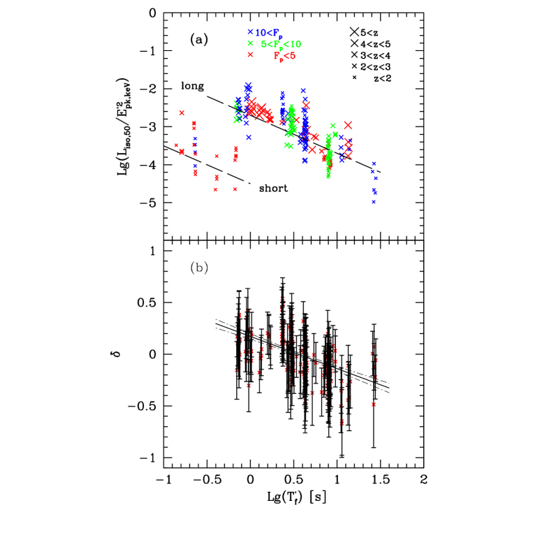
Figure 3: Panel (a): $\mbox{$L_{\rm iso}$}/\mbox{$E_{\rm p}^{\prime}$}^{2}$ vs $T_{f}^{\prime}$ for each burst from the same Swift time–resolved spectral data shown in Fig. 2 and for 9 short Swift GRBs. The size represents the redshift while the colour represents the peak flux in phot cm^-2 s^-1. The dashed lines correspond to a $-1$ slope. Panel (b): Residuals $\delta$ of the correlation $L_{\rm iso}$-$E_{\rm p}^{\prime}$ shown in Fig. 2 and their corresponding uncertainties vs $T_{f}^{\prime}$. The best fit slope $-0.30\pm 0.04$ leads to a scatter reduction term proportional to $\mbox{$T_{f}^{\prime}$}^{1.25\pm 0.20}$.

The thick straight solid line in Fig. 2 is the best linear fit to the logarithmic data performed by a minimum $\chi^{2}$ method taking into account the residual and its uncertainty on the orthogonal direction of the straight line. In Fig. 2 (as well as in the following related Figures), in order to avoid overcrowding, the best fit is plotted only for the Swift sample. The fit gives a line described by:

$${\rm Log}\left(\frac{\mbox{$E_{\rm p}^{\prime}$}}{\rm keV}\right)=a\ {\rm Log}\left(\frac{\mbox{$L_{\rm iso}$}}{10^{b}\ {\rm erg\ s^{-1}}}\right)+c,$$ (3)

The corresponding coefficients of the fits to both the Swift and CGRO samples are given in Tables 3 and 4, respectively (relation LE). Notice that $b$ is not a parameter of the fit, but is the logarithm of $L_{\rm iso}$ in the barycentre of the data–points. The standard errors were computed in the barycentre frame of the data–points in order to minimise any correlation between them. The average correlation slope of both samples is $0.30\pm 0.05$, and the difference in the intercepts at $\mbox{$E_{\rm p}^{\prime}$}=100$ keV between the CGRO and Swift best fits is $0.09\pm 0.11$. We have also estimated the intrinsic scatter $\sigma_{\rm intr}$ of the correlation by adding it iteratively in quadrature to the error in the $y$ axis (Log$E_{\rm p}^{\prime}$) and by requiring that the reduced $\chi^{2}_{r}$ be equal to 1. This method has been tested by Novak et al. (2006) and it gives values similar to those obtained by the fitting method presented in D’Agostini (2005). The intrinsic scatters (standard deviations) around the $E_{\rm p}^{\prime}$ vs $L_{\rm iso}$ correlation for both samples are given in the same Tables 3 and 4. The average value of the $\sigma_{\rm intr}$ is $0.21\pm 0.01$. The dot–dashed lines in Fig. 2 show the intrinsic scatter around the Swift sample correlation.

relation	a	b	c	$\sigma_{\rm intr}$	$\sigma_{\rm intr}^{\rm tot}$
LE	0.25$\pm$0.02	51.48	2.27$\pm$0.02	0.195$\pm$0.013	…
LTE	0.39$\pm$0.02	52.17	2.27$\pm$0.01	0.137$\pm$0.010	…
LTHE	0.49$\pm$0.03	49.48	2.11$\pm$0.02	0.093$\pm$0.020	0.084$\pm$0.007
LTWE	0.66$\pm$0.05	49.42	2.14$\pm$0.02	0.105$\pm$0.020	0.097$\pm$0.008

Table 3: Best–fit slopes $a$ and zero points $c$ of the different logarithmic linear relations studied in this paper for the Swift sample. The parameter $b$ defines the absisa of the barycentre ($10^{b}$, in cgs units) of the given correlation while $\sigma_{\rm intr}$ is the intrinsic scatter. For the correlations which include the collimation angle, $\sigma_{\rm intr}^{\rm tot}$ is an estimate of the scatter contribution due to the internal dispersion of the evolutionary tracks.

relation	a	b	c	$\sigma_{\rm intr}$	$\sigma_{\rm intr}^{\rm tot}$
LE	0.36$\pm$0.03	52.91	2.87$\pm$0.01	0.217$\pm$0.010	…
LTE	0.42$\pm$0.02	53.72	2.88$\pm$0.01	0.174$\pm$0.008	…
LTHE	0.50$\pm$0.02	51.23	2.94$\pm$0.01	0.104$\pm$0.007	0.130$\pm$0.007
LTWE	0.53$\pm$0.02	50.67	2.93$\pm$0.01	0.131$\pm$0.008	0.130$\pm$0.007

Table 4: Same as in Table 3 but for the CGRO sample.

Taking into account the result by Firmani et al. (2006), our next step is to explore a possible correlation of $L_{\rm iso}$ and $E_{\rm p}^{\prime}$ with the high–signal emission rest frame time $T_{f}^{\prime}$. For calculating $T_{f}^{\prime}$, we have taken into account the corrections due to the cosmological time dilation and the narrowing of the light curve’s temporal substructure at higher energies (Fenimore et al. 1995). Following Reichart et al. (2001), this last correction on $T_{f}$, calculated fixing the energy band on the rest frame, goes as $(1+z)^{e}$ with $e\simeq 0.4$. Then applying both corrections we obtain $\mbox{$T_{f}^{\prime}$}=\mbox{$T_{f}$}(1+z)^{-1+e}$ Actually the value of $e$ is not well constrained. For a large BATSE database, Zhang et al. (2007) found that the standard deviation of the distribution of $e$ (modeled as Gaussian) is $0.51$ with a median value of $0.39$; the distribution is skewed to smaller values.

For the Swift sample we find that $L_{\rm iso}$ roughly tends to be $\propto(\mbox{$T_{f}^{\prime}$})^{-1}$ with a large scatter, while $E_{\rm p}^{\prime}$ does not show any significant correlation with $T_{f}^{\prime}$. Now, if we plot $\mbox{$L_{\rm iso}$}/\mbox{$E_{\rm p}^{\prime}$}^{m}$ from each time–resolved spectrum vs $T_{f}^{\prime}$, then the scatter reduces for $m\sim 2$ and a clear trend with slope $-1$ (upper dashed line) is observed (panel (a) of Fig. 3). This result implies that the residuals in the $L_{\rm iso}$–$E_{\rm p}^{\prime}$ diagram (Fig. 2) correlates with $T_{f}^{\prime}$.

It is interesting to show in panel (a) of Fig. 3 the position of some short GRBs with known redshift. We have carried out time resolved spectral analysis for $9$ Swift short GRBs. As seen in Fig. 3, these data are naturally segregated in the diagram, having significantly smaller $\mbox{$L_{\rm iso}$}/\mbox{$E_{\rm p}^{\prime}$}^{2}$ values than those of the long GRBs.

With the aim of checking for possible selection effects behind the correlation presented in panel (a) of Fig. 3, we plot the data with the color code representing the observed peak photon flux ($F_{\rm p}$) range, and with the cross size indicating the redshift range. Our first test has to do with the influence of $F_{\rm p}$ on the $\mbox{$L_{\rm iso}$}/\mbox{$E_{\rm p}^{\prime}$}^{2}$ vs $T_{f}^{\prime}$ diagram. We have divided the sample into three sub-samples: $1.8<\mbox{$F_{\rm p}$}\leq 5$ (red), $5<\mbox{$F_{\rm p}$}\leq 10$ (green), and $\mbox{$F_{\rm p}$}>10$ (blue) (the units are phot cm^-2 s^-1). As seen in Fig. 3, the correlation is remarkably insensitive to the peak flux. In other words the sensitivity limit does not influence the correlation; it only limits the number of objects on it. Our second test refers to a possible bias with $z$. According to the same panel of Fig. 3, it is evident that the data plotted in the $T_{f}^{\prime}$–$\mbox{$L_{\rm iso}$}/\mbox{$E_{\rm p}^{\prime}$}^{2}$ diagram are not appreciably biased by $z$. A third test concerns a possible selection effect on the GRB duration. By plotting $F_{\rm p}$ vs $T_{f}^{\prime}$ for all the Swift GRBs with known $z$ (even those with $\mbox{$F_{\rm p}$}<1.8$ phot cm^-2 s^-1, which were not used in our analysis here), we have seen that the limit $\mbox{$F_{\rm p}$}>1.8$ is well above any biasing limit for $T_{f}^{\prime}$.

Finally, while the upper right side of the diagram in panel (a) of Fig. 3 involves fluxes that are not biased by selection effects, the presence of short GRBs on the bottom left side of the same diagram gives a further evidence against any selection effect here. Unfortunately any further exhaustive analysis on the distribution of $E_{\rm p}$ is impossible due to the limited BAT spectral capability. We conclude that the correlation $\mbox{$L_{\rm iso}$}/\mbox{$E_{\rm p}^{\prime}$}^{2}$ vs $T_{f}^{\prime}$ is reasonably free from selection effects.

Panel (b) of Fig. 3 shows for the Swift sample how much the residuals of the $L_{\rm iso}$–$E_{\rm p}^{\prime}$ diagram of Fig. 2 correlate with $T_{f}^{\prime}$. Here $\delta$ are the orthogonal residuals of the $L_{\rm iso}$–$E_{\rm p}^{\prime}$ best fit (positive $\delta$ correspond to high $L_{\rm iso}$), its standard deviation being calculated in the same direction. The best fit slope of the $\delta$ vs $T_{f}^{\prime}$ correlation is $-0.30\pm 0.04$. Combining this result with the $L_{\rm iso}$–$E_{\rm p}^{\prime}$  best fit slope we obtain that the correlation $E_{\rm p}^{\prime}$ vs $\mbox{$L_{\rm iso}$}\mbox{$T_{f}^{\prime}$}^{p}$ reaches its minimum scatter for $p=1.28\pm 0.20$. A similar analysis on the CGRO sample leads to $p=1.12\pm 0.25$. Given the relevance of this result we have made use of other more sofisticated methods based on multilinear analysis obtaining in each case $p=1.25\pm 0.20$ and $p=1.00\pm 0.20$, respectively. This result implies that the emission time $T_{f}^{\prime}$ of the events on the diagram of Fig. 2 increases along the orthogonal direction of the best fit straight line when one goes from the low $E_{\rm p}^{\prime}$ – high $L_{\rm iso}$ to the high $E_{\rm p}^{\prime}$– low $L_{\rm iso}$. Therefore, as it has been found in Firmani et al. (2006) for a different sample, $T_{f}^{\prime}$  reduces the scatter around the correlation $E_{\rm p}^{\prime}$ vs $L_{\rm iso}$. Later on we will estimate the reduction of such scatter. This result is particularly intriguing because it reveals how instantaneous features such as $L_{\rm iso}$ and $E_{\rm p}^{\prime}$ are actually regulated according to the overall duration of the burst.

We fit the data with the line

$${\rm Log}\left(\frac{\mbox{$E_{\rm p}^{\prime}$}}{\rm keV}\right)=a{\rm Log}\left(\frac{\mbox{$L_{\rm iso}$}\mbox{$T_{f}^{\prime}$}^{p}}{10^{b}{\rm erg\ s^{-1}\ s^{p}}}\right)+c,$$ (4)

where we adopt $p=1.25$ and $p=1$ for the Swift and CGRO samples, respectively. The best linear fit parameters to Eq. (4) for the Swift and CGRO samples are given in Tables 3 and 4, respectively (relation LTE). The average of both slopes is $0.40\pm 0.02$, while the difference in the intercepts at $\mbox{$E_{\rm p}^{\prime}$}=100$ keV between the CGRO and Swift best fits is $0.15\pm 0.07$. The average intrinsic scatter is $\mbox{$\sigma_{\rm intr}$}=0.15\pm 0.02$. A remarkable decrease on the scatter from the $E_{\rm p}^{\prime}$ vs $L_{\rm iso}$ to the $E_{\rm p}^{\prime}$ vs $\mbox{$L_{\rm iso}$}\mbox{$T_{f}^{\prime}$}^{p}$ correlation is evident. Figure 4 shows $E_{\rm p}^{\prime}$ vs $\mbox{$L_{\rm iso}$}\mbox{$T_{f}^{\prime}$}^{p}$ for the same samples plotted in Fig. 2. The best fit line, as in Fig. 2, refers only to the Swift sample, and the corresponding scatter is represented by the dot–dashed lines. Our basic considerations will not change appreciably assuming $p=1$ even for the Swift sample. In fact, the internal scatter changes from $0.137$ to $0.142$ with a standard deviation of $0.010$. The $p=1$ assumption will be taken later on just for economy.

Figure 4: $E_{\rm p}^{\prime}$ vs $L_{\rm iso}$$T_{f}^{\prime}$ for the same time–resolved spectral data shown in Fig. 2. The symbol and line codes are as in Fig. 2. The best–fit line and the $\pm 1\sigma$ intrinsic scatter (solid and dot–dashed lines, respectively) are shown only for the Swift sample.

The previous discussion about selection effects on the diagrams of Fig. 3 can be translated now into the $E_{\rm p}^{\prime}$ vs $\mbox{$L_{\rm iso}$}\mbox{$T_{f}^{\prime}$}^{p}$ correlation (Fig. 4). We conclude then that the latter correlation is reasonably free of selection effects. This is rather evident if we imagine that the effect of $T_{f}^{\prime}$ is to shift the borders of the $E_{\rm p}^{\prime}$ vs $L_{\rm iso}$ correlation into the body of the $E_{\rm p}^{\prime}$ vs $\mbox{$L_{\rm iso}$}\mbox{$T_{f}^{\prime}$}^{p}$ correlation. Then the lack of low luminosity events influences now the population of the $E_{\rm p}^{\prime}$ vs $\mbox{$L_{\rm iso}$}\mbox{$T_{f}^{\prime}$}^{p}$ correlation and not its borders.

Figure 5: The data and lines in the right part of the diagram are the same as those presented in Fig. 2 (the $L_{\rm iso}$$T_{f}^{\prime}$–$E_{\rm p}^{\prime}$ diagram). The data in the left part correspond to the GRBs of both Swift and CGRO samples with known $t_{\rm j}$. For such GRB, $L_{\gamma}$ has been used instead of $L_{\rm iso}$ (the HM case was used to calculate $\theta_{j}$). The symbol and line codes are the same as in Fig. 2. Note how the intrinsic scatter has been reduced by going from the $L_{\rm iso}$$T_{f}^{\prime}$–$E_{\rm p}^{\prime}$ diagram to the $L_{\gamma}$$T_{f}^{\prime}$–$E_{\rm p}^{\prime}$ one.

Figure 6: The data and lines in the right part of the diagram are the same as presented in Fig. 4 (the $L_{\rm iso}$$T_{f}^{\prime}$–$E_{\rm p}^{\prime}$ diagram). The data on the left correspond to the rigid shift of each evolutionary track to best fit with the $E_{\rm p}^{\prime}$ vs $L_{\gamma}$$T_{f}^{\prime}$ correlation for the Swift sub–sample of GRBs with $t_{\rm j}$ known (left part of Fig. 5). The CGRO data are shown only for illustrative purposes; Note that the scatter of the $E_{\rm p}^{\prime}$ vs $L_{\gamma}$$T_{f}^{\prime}$ correlation constructed by the track shifts is only slightly smaller than the one of the original collimation–corrected correlation.

4.2 Scatter reduction by correcting luminosities due to collimation

Following Ghirlanda et al. (2004), a way to reduce the scatter around the $E_{\rm p}^{\prime}$ vs $\mbox{$L_{\rm iso}$}\mbox{$T_{f}^{\prime}$}^{p}$ correlation could be by correcting the time–resolved isotropic luminosities by the jet collimation angle in order to estimate the intrinsic $\gamma-$ray temporal luminosities, $\mbox{$L_{\gamma}$}=(1-\cos\mbox{$\theta_{j}$})\mbox{$L_{\rm iso}$}$. The collimation semi–aperture angle $\theta_{j}$ is calculated from the jet break time $t_{\rm j}$ and the total emitted isotropic energy $E_{\rm iso}$ by two alternative models: the homogeneous ISM model (HM) and the wind medium model (WM). Unfortunately, reliable estimates of $t_{\rm j}$ for our GRB sample are available only for some events. We use the $t_{\rm j}$ values compiled from the literature by Ghirlanda et al. (2007). Our GRBs with known $t_{\rm j}$ reduces to 7 events of Swift with 37 time resolved spectra, and 5 of CGRO with 195 time resolved spectra (see Tables 1 and 2).

In the HM model, the jet opening angle is given by:

$$\mbox{$\theta_{j}$}=0.161{\left({\frac{\mbox{$t_{\rm j}$}_{,d}}{1+z}}\right)}^{3/8}\left({\frac{n\eta_{\gamma}}{\mbox{$E_{\rm iso}$}_{,52}}}\right)^{1/8},$$ (5)

where $\eta_{\gamma}$ is the radiative efficiency that we assume equal to 0.2, and $n$ is the medium density that we assume equal to 3 cm^-3.

Figure 5 shows the collimation–corrected correlation $E_{\rm p}^{\prime}$ vs. $L_{\gamma}$$T_{f}^{\prime}$ for 12 GRB with known $t_{\rm j}$ (left correlation), together with the same data presented in Fig. 4 (right correlation). The best fit line showed for the collimation–corrected correlation refers only to the Swift sample; the corresponding scatter is represented by the dot–dashed lines. Fitting the data with the line

$${\rm Log}\left(\frac{\mbox{$E_{\rm p}^{\prime}$}}{\rm keV}\right)=a{\rm Log}\left(\frac{\mbox{$L_{\gamma}$}\mbox{$T_{f}^{\prime}$}}{10^{b}{\rm erg}}\right)+c$$ (6)

the best fit parameters of the $E_{\rm p}^{\prime}$ vs $L_{\gamma}$$T_{f}^{\prime}$ correlations (HM case) for Swift and CGRO samples are given in Tables 3 and 4, respectively (relation LTHE). The slopes of both correlations are very close, the average being $0.50\pm 0.03$. Concerning the scatter, for both samples $\sigma_{\rm intr}$ has clearly reduced its value with respect to the one in the $E_{\rm p}^{\prime}$ vs $L_{\rm iso}$$T_{f}^{\prime}$ correlations; on average we find $\mbox{$\sigma_{\rm intr}$}=0.10\pm 0.01$.

We conclude that the HM collimation angle introduces a remarkable reduction on the scatter in the $E_{\rm p}^{\prime}$ vs $L_{\rm iso}$$T_{f}^{\prime}$ correlation. However, such a reduction does not concern the internal scatter in each GRB evolutionary track.

In order to estimate the contribution of the internal scatter from each evolutionary track to the overall correlation intrinsic scatter, we have performed the following exercise. For each sample (Swift  or CGRO), every $L_{\rm iso}$$T_{f}^{\prime}$–$E_{\rm p}^{\prime}$ GRB track is shifted rigidly to best fit with the collimation–corrected correlation $E_{\rm p}^{\prime}$ vs $L_{\gamma}$$T_{f}^{\prime}$ presented above for the corresponding sample (see Fig. 6 for the Swift sample; here the evolutionary tracks of the CGRO GRBs are included only for graphic display). We are now able to calculate the new intrinsic scatter of the corresponding sample, $\sigma_{\rm intr}^{\rm tot}$, around the respective correlation $E_{\rm p}^{\prime}$ vs $L_{\gamma}$$T_{f}^{\prime}$. The values of $\sigma_{\rm intr}^{\rm tot}$ (relation LTHE) are reported in Tables 3 and 4 for the Swift and CGRO samples, respectively. By comparing $\sigma_{\rm intr}$ and $\sigma_{\rm intr}^{\rm tot}$, it is rather evident that the scatter of the tight collimation–corrected correlation is dominated by the internal scatter of the evolutionary tracks. A similar result is obtained if instead of the entire sample we estimate the $\sigma_{\rm intr}^{\rm tot}$ taking into account the GRB with the known jet break time alone. In fact in this case the average internal scatter is $\mbox{$\sigma_{\rm intr}^{\rm tot}$}=0.08\pm 0.01$. We conclude that any further reduction of the collimation–corrected correlation scatter could be reached by reducing the internal scatter of each evolutionary track, and that the latter should be possibly identifying the hidden parameters behind the stochastic properties of the evolutionary tracks of each GRB.

In the WM model the jet opening angle is given by

$$\mbox{$\theta_{j}$}=0.202{\left({\frac{\mbox{$t_{\rm j}$}_{,d}}{1+z}}\right)}^{1/4}\left({\frac{A_{\ast}\eta_{\gamma}}{\mbox{$E_{\rm iso}$}_{,52}}}\right)^{1/4},$$ (7)

where now the medium density is supposed to be $n\left(r\right)=5\times 10^{11}A_{\ast}r^{-2}$ g cm^-1 and we assume $A_{\ast}=1$. Tables 3 and 4 present the corresponding best fit parameters for the $E_{\rm p}^{\prime}$ vs $L_{\gamma}$ $T_{f}^{\prime}$ correlation in the WM case (relation LTWE). In this case the best fit slopes are moderately close ($95\%$ CL). The average of both slopes is $0.60\pm 0.05$. The scatters $\sigma_{\rm intr}$ of the WM collimation–corrected correlations are also smaller than the ones of the not corrected correlations $E_{\rm p}^{\prime}$ vs $L_{\rm iso}$$T_{f}^{\prime}$, but the scatter reduction is smaller than in the HM case. On average we find $\mbox{$\sigma_{\rm intr}$}=0.12\pm 0.01$. After performing the same track shifting procedure described above, we find that also in this case the internal scatter of each GRB evolutionary track provides the dominant component of the scatter around the tight $E_{\rm p}^{\prime}$ vs $L_{\gamma}$$t_{\rm j}$ correlation.

Finally, we have explored whether the residuals of the $L_{\rm iso}$$T_{f}^{\prime}$–$E_{\rm p}^{\prime}$  correlation correlate or not with several prompt light–curve parameters: the variability $V$ (Reichart et al. 2001); the ”emission symmetry” $S_{F}=T_{2}/T_{1}$, where $T_{1}$ and $T_{2}$ are the duration times of the fluence–halves, from $5-50\%$ and $50-95\%$ of the total counts, respectively (Borgonovo & Björnsson 2006); the $\mbox{$E_{\rm p}$}^{(1)}/\mbox{$E_{\rm p}$}^{(2)}$ ratio, where $\mbox{$E_{\rm p}$}^{(1)}$ and $\mbox{$E_{\rm p}$}^{(2)}$ are the peak energies of the integrated $\nu f_{\nu}$ spectra for each of the two time intervals $T_{1}$ and $T_{2}$, respectively (Borgonovo & Björnsson 2006). Our preliminary results show that the residuals are not correlated with any of these parameters, i.e. none of them could be a potential reductor of the scatter around the $L_{\rm iso}$$T_{f}^{\prime}$–$E_{\rm p}^{\prime}$  correlation.

5 Conclusions

We have selected the high–signal time–resolved spectra from the available sample of Swift long GRBs with measured $z$, and analysed them with the aim to search for systematic features of the local $\gamma-$ray emission mechanism and their connection with known global GRB properties. Requiring a GRB peak flux $\mbox{$F_{\rm p}$}>1.8$ phot cm^-2 s^-1, a total of 207 time–resolved spectra corresponding to 32 GRBs (until February 2008) were analysed. We have included also 287 spectra from 7 bright CGRO GRBs with $z$ known analysed previously in Kaneko et al. (2006). Since the two samples are affected in a different way by some systematic effects, we preferred to perform our correlation analysis separately for each sample and then to check whether the results are consistent or not between them. We have found that they are indeed consistent. Thus, for simplicity, in what follows we report the averages of the two samples for the best–fit parameters of the different correlations.

The main results and conclusions from our study are as follows:

• By plotting the time–resolved data–points in the logarithmic $L_{\rm iso}$–$E_{\rm p}^{\prime}$ diagram, a linear band with average slope $0.30\pm 0.05$ and intrinsic scatter $\mbox{$\sigma_{\rm intr}$}=0.21\pm 0.01$ appears. While the low $E_{\rm p}^{\prime}$ – high $L_{\rm iso}$ region is free of selection effects, the high $E_{\rm p}^{\prime}$– low $L_{\rm iso}$  region could be affected by the flux limits of the samples.

• We found that the residuals in the $L_{\rm iso}$–$E_{\rm p}^{\prime}$ diagram correlate with $T_{f}^{\prime}$. This result offers a strong evidence that the parameter $T_{f}^{\prime}$ reduces the scatter of the $E_{\rm p}^{\prime}$ vs $L_{\rm iso}$ correlation. By analyzing the $T_{f}^{\prime}$ vs $\mbox{$L_{\rm iso}$}/\mbox{$E_{\rm p}^{\prime}$}^{2}$ diagram (Fig. 3), we have checked that selection effects are not responsible for such a trend.

• In agreement with the previous point, we have introduced the logarithmic diagram $E_{\rm p}^{\prime}$ vs $\mbox{$L_{\rm iso}$}\mbox{$T_{f}^{\prime}$}^{p}$ and have found that the optimal value $p=1.1\pm 0.1$ reduces the scatter to $\mbox{$\sigma_{\rm intr}$}=0.15\pm 0.02$. The average slope of the correlation is $0.40\pm 0.02$. Such correlation reveals three important aspects. First, its intrinsic scatter is smaller than the intrinsic scatter in the $E_{\rm p}^{\prime}$ vs $L_{\rm iso}$ correlation. Second, it is reasonably free from selection effects, accordying to our our analysis in the $T_{f}^{\prime}$ vs $\mbox{$L_{\rm iso}$}/\mbox{$E_{\rm p}^{\prime}$}^{2}$ diagram. Third, it represents a connection between instantaneous features ($E_{\rm p}^{\prime}$, $L_{\rm iso}$) and global features ($T_{f}^{\prime}$). At any moment, the instantaneous features of a GRB correlate with the entire prompt duration as if at each instant of the prompt the GRB would be aware of the duration of the entire process.

• For the 12 GRBs out of our samples (7 from the Swift and 5 from the CGRO samples, respectively) for which the jet break time $t_{\rm j}$ is known, we could further reduce the scatter of each sample by using the collimation–corrected luminosity $L_{\gamma}$ by estimating the collimation jet angle for the homogeneous (HM) and wind medium (WM) cases. The lowest intrinsic scatter has been obtained for the $E_{\rm p}^{\prime}$ vs $L_{\gamma}$$T_{f}^{\prime}$ correlation in the HM case; the (average) slope of the correlation is $0.50\pm 0.03$ and $\mbox{$\sigma_{\rm intr}$}=0.10\pm 0.01$.

• We have estimated the contribution of the internal scatter of the evolutionary tracks to the scatter of the overall correlations. For this, the $L_{\rm iso}$–$E_{\rm p}^{\prime}$ evolutionary track of each GRB has been shifted to best fit with the corresponding collimation–corrected (HM and WM cases) correlations. Our results indicate that for both cases $\mbox{$\sigma_{\rm intr}$}\approx\mbox{$\sigma_{\rm intr}^{\rm tot}$}$, this means that the total intrinsic scatter is mainly due to the internal scatter of the tracks. Thus, with the caveat that the statistics is still limited, we conclude that any further reduction of the scatter around the GRB empirical correlations may be attained by discovering the hidden variables behind the stochastic features of the individual $E_{\rm p}^{\prime}$–Liso evolutionary tracks.

We conclude that the long GRB individual evolutionary tracks populate a rather narrow strip in the $E_{\rm p}^{\prime}$ vs $L_{\rm iso}$$T_{f}^{\prime}$ diagram with a slope $\approx 0.4$, whatever the evolutionary track slope is. The jet collimation correction further reduces the thickness of such strip and leads the slope close to $0.5$. While selection effects probably are present in the $E_{\rm p}^{\prime}$ vs $L_{\rm iso}$ diagram, they do not seem to weaken our conclusion. This implies the existence of a universal $\gamma$–ray emission mechanism for long GRBs where the instantaneous features are modulated by a global parameter, which we found here to be $T_{f}^{\prime}$. We suggest that the interconnection between $T_{f}^{\prime}$ and the $L_{\rm iso}$–$E_{\rm p}^{\prime}$ evolutionary tracks is at the basis of the global ‘Amati’ and ‘Ghirlanda’ relations.

References

- [Amati et al.(2002)] Amati, L., et al. 2002, A&A, 390, 81
- [Band et al.(1993)] Band D., Matteson J., Ford L., et al., 1993, ApJ, 413, 281
- [Borgonovo & Ryde(2001)] Borgonovo, L. & Ryde, F. 2001, ApJ, 548, 770
- [Borgonovo & Björnsson(2006)] Borgonovo, L., & Björnsson, C. I. 2006, ApJ, 652, 1423
- [Cabrera et al.(2007)] Cabrera, J.I., Firmani, C., Avila-Reese, V., Ghirlanda, G., Ghisellini, G., & Nava, L., 2007, MNRAS, 382, 342
- [Collazzi & Schaefer] Collazzi, A. C., & Schaefer, B. E. 2008, ArXiv e-prints, 808, arXiv:0808.2061
- [D’Agostini(2005)] D’Agostini, G. 2005, preprint (arXiv:physics/0511182)
- [Fenimore et al.(1995)] Fenimore, E. E., in ’t Zand, J. J. M., Norris, J. P., Bonnell, J. T., Nemiroff, R. J. 1995, ApJL, 448, L101
- [Firmani et al.(2006)] Firmani C., Ghisellini G., Avila–Reese V. & Ghirlanda G., 2006, MNRAS, 370, 185
- [] Genet, F., Daigne, F. & Mochkovitch, R., 2007, MNRAS, 381, 732
- [Gehrels et al.(2004)] Gehrels, N. et al. 2004, ApJ, 611, 1005
- [Ghirlanda et al.(2004)] Ghirlanda, G., Ghisellini, G. & Lazzati, D. 2004, ApJ, 616, 331
- [Ghirlanda et al.(2006)] Ghirlanda, G., Ghisellini, G., & Firmani, C., 2006, New Journal of Physics, 8, 123
- [Ghirlanda et al.(2007)] Ghirlanda, G., Nava, L., Ghisellini, G., & Firmani, C., 2007, A&A, 466, 127
- [] Ghisellini, G., Ghirlanda, G., Nava, L. & Firmani, C., 2007, ApJ, 658, L75
- [Kaneko et al.(2006)] Kaneko, Y., Preece, R.D., Briggs, M.S., Paciesas, W.S., Meegan, C.A. & Band, D.L., 2006, ApJSS, 166, 298
- [Kann et al.(2008)] Kann, D.A., Schulze, S. & Updike, A.C. 2008, GRB Coordinates Network, 7627, 1
- [Liang & Zhang(2005)] Liang E. & Zhang B., 2005, ApJ, 633, 611
- [Liang et al.(2004)] Liang, E.W., Dai, Z.G., & Wu, X.F., 2004, ApJL, 606, L29
- [Meszaros(2006)] Mészáros, P. 2006, Reports of Progress in Physics, 69, 2259
- [Novak et al.(2006)] Novak, G.S., Faber, S.M., & Dekel, A., 2006, ApJ, 637, 96
- [Preece et al.(2000)] Preece, R.D., Briggs, M.S., Mallozzi, R.S., Pendleton, G.N., Paciesas, W.S. & Band, D.L., 2000, ApJSS, 126, 19
- [Rossi et al.(2008)] Rossi, F., et al., 2008, MNRAS, 388, 1284
- [Ryde & Petrosian(2002)] Ryde, F., & Petrosian, V., 2002, ApJ, 578, 290
- [Thompson, Rees & Mészáros(2007)] Thompson, C., Rees, M.J. & Mészáros, P., 2007, ApJ, 666, 1012
- [] Uhm, Z.L. & Beloborodov, A.M., 2007, ApJ, 665, L93
- [Yonetoku et al.(2004)] Yonetoku, D., Murakami, T., Nakamura, T., Yamazaki, R., Inoue, A.K., & Ioka, K., 2004, ApJ, 609, 935
- [Zhang (2007)] Zhang, B. 2007, Chin. J. Astron. Astrophys., 7, 1