Transonic properties of the accretion disk around compact objects

An accretion flow is necessarily transonic around a black hole. However, around a neutron star it may or may not be transonic, depending on the inner disk boundary conditions influenced by the neutron star. I will discuss various transonic behavior of the disk fluid in general relativistic (or pseudo general relativistic) framework. I will address that there are four types of sonic/critical point possible to form in an accretion disk. It will be shown that how the fluid properties including location of sonic points vary with angular momentum of the compact object which controls the overall disk dynamics and outflows.

1 Introduction

Accretion disks serve to identify compact objects, mostly black holes and neutron stars, in the universe. The most common way to understand its formation is in a binary system where matter is pulled off a companion star and settles on to the compact object in the form of a disk. As practically black holes and neutron stars cannot be seen, by detecting and analyzing light rays off an accretion disk one can understand the properties of the central compact object. Other examples of the accretion disk are the protoplanetary disks, disks around active galactic nuclei, in star-forming systems, and in quiescent cataclysmic variables etc.

The molecular viscosity in an accretion disk is rather low. Shakura & Sunyaev ss73 proposed that there is a significant turbulent viscosity explaining transport of matter inwards and angular momentum outwards with the Keplerian angular momentum profile pringle . However, until the work by Balbus & Hawley bh origin of the instability and plausible turbulence was not understood. Applying the idea of Magneto-Rotational-Instability (MRI) described by Velikhov vel59 and Chandrasekhar chandra60 , they showed that the Keplerian disk flow may exhibit unstable modes under perturbation in the presence of a weak magnetic field. This plausibly generates turbulence which results transport. However, there are several accretion disk systems where gas is electrically neutral in charge and thus the magnetic field does not couple with the system. Examples of such system are protoplanetary and star-forming disks, disks around active galactic nuclei and in quiescent cataclysmic variables. Hence in these systems MRI is expected not to work to generate turbulence. While the origin of the transport in such systems is still an ill understood problem, some mechanisms have been proposed by various groups including the present author tev ; yek ; um04 ; mukh05a ; mukh05b ; mukh06 ; zahn .

However, the problems of the transport and then the viscosity are not severe if the disk angular momentum profile deviates from the Keplerian type to sub-Keplerian type. In a sub-Keplerian disk, the gravitational force dominates over the centrifugal force resulting in a strong advective component of the infalling matter abrazur ; c89 ; ny . Due to the dominance of the gravity, the matter even with a constant angular momentum may transport inwards easily. An accretion disk with a strong advective component, namely the advective accretion disk, is hotter than the Keplerian disk which explains successfully several systems e.g. Sgr $A^{*}$, GRS 1515+105 which are expected to be consisting of hot disks. Therefore, such an accreting system may not be of pure Keplerian type. At least close to the compact object it is an advective accretion disk. In a sub-Keplerian disk, at far away off the black hole, the speed of the infalling matter is close to zero when it is practically out of the black hole’s influence. However, temperature of the system is finite resulting in finite sound speed at that radius. On the other hand, matter speed at the black hole horizon reaches the speed of light ($c$), while, by causality condition, sound speed can be at the most $c/\sqrt{3}$. Therefore, there must be a location where matter speed crosses local sound speed making the flow transonic. However, the second condition namely the inner boundary condition not necessarily be satisfied in the flow around a neutron star. Therefore an accretion flow around a neutron star may or may not be transonic.

In the present article, I mainly concentrate on the sub-Keplerian accretion disk with possible multitransonic flow. If the flow is transonic, then the disk dynamics and corresponding outflow are influenced by the sonic locations/points c89 ; c96r ; c99 ; m03 ; mg03 . Depending upon the flow energy (entropy) and angular momentum, a disk may exhibit one to four sonic points, through which all however, matter may not pass. Sonic points in accretion disks play role similar to the critical points in simple harmonic oscillators, particularly to control the dynamics of the system. Indeed an accretion disk can be looked upon as a damped harmonic oscillator c90 .

I organize the paper as follows. In the next section, I discuss accretion flow, first the spherical one and then the disk flow, and formation of possible sonic points therein in the absence of any energy dissipation. In §3, I analyze how the rotation of the compact object affects the sonic points. Subsequently, for completeness, I present the generalized set of accretion disk equations including possible dissipation effects in §4, without going into their solutions. Finally, I summarize in §5.

2 Accretion flow and formation of sonic points

First I discuss simple spherical accretion namely Bondi flow. Subsequently, I include angular momentum into the equations set describing disk accretion. I show that while the Bondi flow around a nonrotating compact star exhibits single sonic point the disk flow may exhibit multiple sonic points.

As gravity is expected to be very strong close to the compact object, in principle I should describe the flow system by the set of general relativistic equations. For a nonrotating compact object equations should be written in the Schwarzschild geometry and for a rotating compact object they should be in the Kerr geometry. However, that might hide transparency of the description, as the full general relativistic set of equations is so cumbersome that it is difficult to relate the terms with the physics they carry. Indeed under some occasions a full general relativistic description is not required. Therefore, I describe the system by pseudo-Newtonian approach. Here one uses Newtonian set of equations only along with a modified gravitational force/potential such that it mimics the general relativistic features approximately to describe the system.

2.1 Bondi flow

This happens for an isolated star when matter falls onto it from all directions, resulting in a spherical accretion. Therefore, to describe the system, we consider the spherical polar coordinate system where only nonzero component of velocity is $v_{r}=v$. Hence the equations describing the steady-state flow with negligible viscosity are given as:

$$v\frac{dv}{dx}+\frac{1}{\rho}\frac{dP}{dx}+F_{g}=0,$$ (1)

$$\frac{1}{x^{2}}\frac{d}{dx}\left(\rho vx^{2}\right)=0,{\rm\,\,\,hence\,\,\,}\rho vx^{2}={\rm constant}=\dot{M}_{ac},$$ (2)

where all the variables are expressed in dimensionless units. $v$ is velocity in unit of light speed, $x=r/r_{g}$ where $r$ is radial coordinate and $r_{g}=GM_{s}/c^{2}$, $M_{s},c,G$ are respectively mass of the central star, speed of light, Newton’s gravitation constant, $P,\rho$ are respectively corresponding dimensionless pressure, density of the flow, $\dot{M}_{ac}$ is accretion rate and $F_{g}$ is gravitational force given by

$$F_{g} = \frac{1}{x^{2}}:\,\,{\rm Newtonian},$$ (3)

$$= \frac{1}{(x-2)^{2}}:\,\,{\rm pseudo-Newtonian,\,\,Schwarzschild\,\,geometry}\,\cite[cite]{\@@bibref{Authors Phrase1YearPhrase2}{pw}{\@@citephrase{(}}{\@@citephrase{)}}},$$ (4)

$$= \frac{(x^{2}-2j\sqrt{x}+j^{2})^{2}}{x^{3}(\sqrt{x}(x-2)+j)^{2}}:\,\,{\rm pseudo-Newtonian,\,\,Kerr\,\,geometry}\,\cite[cite]{\@@bibref{Authors Phrase1YearPhrase2}{m02}{\@@citephrase{(}}{\@@citephrase{)}}},$$ (5)

where $j$ is specific angular momentum of the compact object. Integrating equation (1) for an adiabatic flow to a nonrotating compact object I obtain

$$E=\frac{1}{2}v^{2}+na^{2}-\frac{1}{x-2},$$ (6)

where polytropic index $n=1/(\gamma-1)$ and $\gamma$ is defined as $\gamma=a^{2}\rho/P$ with $P=K\rho^{\gamma}$, $K$ is gas constant and $a$ is sound speed. If the Mach number of the flow is defined as $M=v/a$, then at a constant energy $E$, it is clearly understood from (6) that $M-x$ trajectory is always hyperbolic-type bondi with a sonic point at $M=1$ shown in Fig. 1 c90 . The solution marked ‘A’ by an arrow indicates accretion and marked ‘C^′’ as wind. None of the other solutions are physical to describe accretion and wind. However, for the flow around a rotating compact object, there might be more than one sonic point but I will not discuss them here, this can be checked with a pseudo-Newtonian potential proposed for the Kerr geometry m02 .

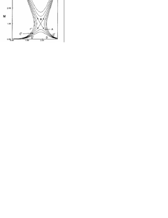
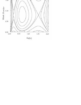
Figure 1: Upper panel: Bondi flow: Mach number as a function of logarithmic radial coordinate for various energy of the flow. The point ‘B’ is sonic point and the solution marked by the arrow ‘A’ indicates accretion and ‘C^′’ indicates wind. Lower panel: Disk flow: Same as Bondi flow; c90 .

2.2 Disk accretion flow

Now I consider a binary system when the compact object is closely associated with its binary companion star and pulling matter off it. The gravitational force acts on the donor star radially. On the other hand, the star is rotating and hence the matter detached off it due to gravitational pull has angular momentum. As a result the matter infalls towards the compact object in a spiral path forming a disk around it called the accretion disk. Therefore, the radial momentum balance equation describing disk dynamics in steady-state in the absence of any energy dissipation is m03

$$v\frac{dv}{dx}+\frac{1}{\rho}\frac{dP}{dx}-\frac{\lambda^{2}}{x^{3}}+F_{g}=0,$$ (7)

where $\lambda$ is specific angular momentum of the infall which is a conserved quantity in a nondissipative flow. The corresponding vertically averaged mass conservation reads as

$$\frac{1}{x}\frac{d}{dx}\left(x\Sigma v\right)=0,\,\,{\rm hence}\,\,-4\pi x\Sigma v={\rm constant}=\dot{M}_{ac},$$ (8)

where $\Sigma\sim h(x)\rho$ is the (vertically integrated) column density matsum with $\rho$ is density at the equatorial plane, $h(x)=a\sqrt{x/F_{g}}$ is the half-thickness of the disk computed from the assumption of vertical equilibrium. Now integrating (7) for an adiabatic flow towards a nonrotating compact object I obtain specific energy of the flow

$$E=\frac{1}{2}v^{2}+na^{2}+\frac{\lambda^{2}}{2x^{2}}-\frac{1}{x-2},$$ (9)

which is a conserved quantity for the nondissipative system. It is seen from (9) that at far away from the black hole and close to its event horizon located at $x=2$, last term (gravitational potential energy) on the right hand side dominates over the last but one term (centrifugal energy) resulting in a hyperbolic-type $M-x$ trajectory as shown in Fig. 1 c96r ; c90 . On the other hand, at an intermediate location, with an appropriate value of $\lambda$, centrifugal energy may dominate over gravitational potential energy resulting in an ellipse-type $M-x$ trajectory as shown in Fig. 1.

2.3 Formation of sonic points in disk accretion

Combining (7) and (8) I obtain

$$\frac{dv}{dx}=\frac{\frac{\lambda^{2}}{x^{3}}-F_{g}+\frac{a^{2}}{\gamma+1}\left(\frac{3}{x}-\frac{1}{F_{g}}\frac{dF_{g}}{dx}\right)}{v-\frac{2a^{2}}{(\gamma+1)v}}=\frac{N}{D}.$$ (10)

At the sonic point $x=x_{c}$, $D=0$ and thus to have continuous $dv/dx$ at the same location $N$ must vanish. Hence, applying $N=D=0$ at $x=x_{c}$ to (10), I obtain velocity, sound speed, specific energy at $x_{c}$

$$v_{c} = a_{c}\sqrt{\frac{2}{\gamma+1}},\,\,{\rm hence\,\,Mach\,\,number}\,\,M_{c}=\sqrt{\frac{2}{\gamma+1}},$$

$$a_{c} = \sqrt{(\gamma+1)\left(\frac{\lambda^{2}}{x_{c}^{2}}-F_{gc}\right)\left[\frac{1}{F_{gc}}\left(\frac{dF_{g}}{dx}\right)_{c}-\frac{3}{x_{c}}\right]^{-1}},$$

$$E_{c} = \frac{2\gamma}{\gamma-1}\left[\frac{\frac{\lambda^{2}}{x_{c}^{3}}-F_{gc}}{\frac{1}{F_{gc}}\left(\frac{dF_{g}}{dx}\right)_{c}-\frac{3}{x_{c}}}\right].$$ (11)

I also compute a quantity that carries information of entropy

$$\dot{\cal M}=(\gamma K)^{n}\dot{M}_{ac}$$ (12)

which is a useful quantity to study the sonic point behavior. Now to obtain solutions for the accretion disk one has to integrate (10) with a proper boundary condition. As our interest is in transonic solutions, the matter necessarily passes through the sonic location and this I consider as our staring point of the integration. As the system under consideration is in the steady-state, integrating from the sonic point to outwards (inwards) and vice versa are equivalent. However, $dv/dx$ given in (10) is of $0/0$ form. Therefore, applying l’Hospital’s rule, I obtain $dv/dx$ at $x=x_{c}$

$$\left(\frac{dv}{dx}\right)_{c}=-\frac{{\cal B}+\sqrt{{\cal B}^{2}-4{\cal A}{\cal C}}}{2{\cal A}},$$ (13)

where,

$${\cal A} = 1+\frac{2a_{c}^{2}}{(\gamma+1)v_{c}^{2}}+\frac{4a_{c}^{2}(\gamma-1)}{v_{c}^{2}(\gamma+1)^{2}},$$

$${\cal B} = \frac{4a_{c}^{2}(\gamma-1)}{v_{c}(\gamma+1)^{2}}\left[\frac{3}{x_{c}}-\frac{1}{F_{gc}}\left(\frac{dF_{g}}{dx}\right)_{c}\right],$$

$${\cal C} = \frac{a_{c}^{2}}{\gamma+1}\left[\left(\frac{1}{F_{gc}}\left(\frac{dF_{g}}{dx}\right)_{c}\right)^{2}-\frac{1}{F_{gc}}\left(\frac{d^{2}F_{g}}{dx^{2}}\right)_{c}-\frac{3}{x_{c}^{2}}\right]$$ (14)

$$- \frac{3\lambda^{2}}{x_{c}^{4}}-\left(\frac{dF}{dx}\right)_{c}-\frac{a_{c}^{2}(\gamma-1)}{(\gamma+1)^{2}}\left[\frac{3}{x_{c}}-\frac{1}{F_{gc}}\left(\frac{dF_{g}}{dx}\right)_{c}\right]^{2}.$$

Now the value of discriminant ${\cal D}={\cal B}^{2}-4{\cal A}{\cal C}$ determines the type of sonic point. Clearly ${\cal D}$ depends on the sonic location which can be computed for a given $E_{c}$ from (11). In fact, the expression for $E_{c}$ can be rewritten as a fourth order polynomial of $x_{c}$. Hence, $E_{c}$ and $\lambda$ are the input parameters determining flow behavior for a given system.

There are four different types of sonic point shown in Fig. 2 st ; c90 classified according to the trajectory around it. (1) When ${\cal D}<0$ with ${\cal B}=0$, sonic point is center-type (elliptical trajectories in Fig. 1). (2) ${\cal D}<0$ with ${\cal B}\neq 0$ gives spiral-type sonic point. For ${\cal D}\geq 0$ with (3) ${\cal AC}>0$ it is nodal-type, and (4) ${\cal AC}<0$, saddle-type (hyperbolic trajectories in Figs. 1). When ${\cal AC}=0$ for ${\cal D}\geq 0$, sonic points are called straight line.

Figure 2: Trajectories around various critical points where abscissa and ordinate are radial coordinate and Mach number respectively; c90 ; st .

3 Sonic point analysis in disks around rotating compact objects

The energy and information of entropy at the sonic point $E_{c}$ and $\dot{\cal M}_{c}$ as functions of sonic location $x_{c}$ given by (11) and (12) respectively describe the loci of sonic point energy and entropy of the flow. Figure 3 m03 shows their behavior for various choice of specific angular momentum of the compact object. As I consider a nondissipative disk, the energy and entropy remain conserved throughout. The intersections of the curves by the constant energy and entropy line (which are the horizontal lines in the figure) indicate the sonic points of the accretion disk for that particular energy and entropy and specific angular momentum of the black hole (Kerr parameter). It is clearly seen that, at a particular energy and entropy, if the Kerr parameter increases, the region where sonic points form (as well as radii of marginally bound ($x_{b}$) and stable ($x_{s}$) orbits) shift(s) to a more inner region of the disk and possibility to have all sonic points in the disk outside event horizon increases. As an example, for $a=0.998$, the inner edge of the accretion disk enlarges to such an extent that the fourth sonic point in the disk appears outside the event horizon. On the other hand, for retrograde orbits (counter rotating cases), all the sonic points come close to each other tending to overlap for a particular value of the Kerr parameter (when $x_{b}$ and $x_{s}$ move to greater radii). Therefore, as the value of the Kerr parameter decreases, the possibility of forming individual sonic points decreases and thus shrinking the region containing sonic points. This is very well-understood physically; as the Kerr parameter decreases, total angular momentum of the system decreases resulting in the disk tends to a Bondi-like flow, that has single saddle-type sonic point.

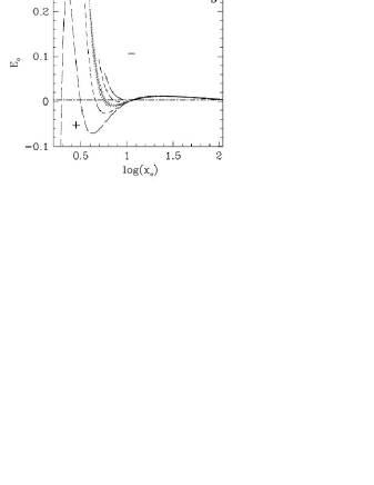
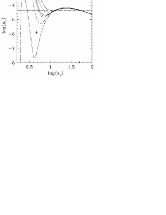
Figure 3: Variation of energy (upper panel) and information of entropy (lower panel) as functions of logarithmic sonic radius when $j$ is a parameter. Central solid curve is for nonrotating compact object ($j=0$), while curves in regions of either side of it indicated by ‘$+$’ and ‘$-$’ are for prograde and and retrograde orbits respectively. Different curves from $j=0$ line to downwards are for $j=0.1,0.5,0.998$ and to upwards for $j=-0.1,-0.5,-0.998$. The horizontal line indicates the curve of constant energy of $0.0065$ (upper panel) and of constant entropy of $5\times 10^{-5}$ (lower panel). Other parameters are $\lambda=3.3$, $\gamma=4/3$; m03 .

On the other hand, for a particular $a$, if $E_{c}$ and $\dot{\cal M}_{c}$ decrease, then the possibility to have all the sonic points in the disk increases. This is understood from Fig. 3 that as $E_{c}$ and $\dot{\cal M}_{c}$ decrease, the curve is more likely to intersect the horizontal line. If $E_{c}=0.05$, then number of intersection of all the curves, except the dashed one, by the $E_{c}=0.05$ line is one giving only sonic point. The dashed curve with $a=0.998$ intersects twice. However, for $E_{c}=0.0065$ (as considered in Fig. 3), the dashed curve intersects four times exhibiting four possible sonic points in the flow and the other curves intersect thrice. For a detailed description, see earlier works m03 ; mg03 .

Note that the sonic points occurring with a negative slope of the curve indicate the locations of ‘saddle-type’ sonic point and those with a positive slope indicate the ‘center-type’ sonic point. Thus the rotation of a black hole plays an important role in the formation of the sonic points which are related to the structure of accretion disks and presumably formation of outflows and jets.

4 Generalized set of equations describing a sub-Keplerian accretion disk

So far, for simplicity, I have described disks without any dissipative energy. In principle a disk must exhibit viscous dissipation making angular momentum varying with disk radius. The hot disk flow with ion temperature $T\geq 10^{9}$K is also expected to generate significant nuclear energy mostly via proton-capture reactions mc99 ; mc00 . On the other hand, significant energy is radiated out through the inverse-Compton, bremsstrahlung and synchrotron effects, cooling the disk. In addition, significant energy is expected to be absorbed through endothermic nuclear reactions, mostly via dissociation of elements mc99 ; mc00 ; mc01 , affecting disk dynamics significantly. Although the main purpose of the paper is to describe the basic mechanism to form sonic points in accretion disks and for that the inviscid set of equations without dissipation suffices, for completeness here I describe the generalized set of equations including effects of energy dissipation. However, I will not go for the solutions of such equations set which is beyond the scope of present paper.

Therefore, in general one should incorporate two more equations namely angular momentum balance and energy equation apart from (7) and (8) as given below. I express viscous dissipation $q^{+}$ in terms of shear stress $W_{x\phi}$ as $q^{+}=W_{x\phi}^{2}/\eta$, where $\eta$ is the coefficient of viscosity. Shakura & Sunyaev ss73 parametrized shear stress in a Keplerian disk by gas pressure with a constant $\alpha$, called Shakura-Sunyaev viscosity parameter, such that $W_{x\phi}=-\alpha P$. However, in an advective disk, there must be a significant contribution due to ram pressure and thus shear stress may be read as $W_{x\phi}=-\alpha(I_{n+1}P+I_{n}v^{2}\rho)h(x)$, where I consider vertically averaged disk and $I_{n+1},I_{n}$ appear due to integration in the vertical direction matsum when $P$ and $\rho$ are pressure and density respectively at the equatorial plane. However, if I use this expression of shear stress in describing $q^{+}$, it loses information of actual shear, effect due to variation of angular velocity in the disk. The proper way of writing shear stress should be $W_{x\phi}=\eta x\frac{d\Omega}{dx}$, where $\Omega$ is angular frequency of the flow. If I substitute this into $q^{+}$, then final equation to be solved will contain a nonlinear derivative term making it tedious to solve. Therefore, following Chakrabarti c96 , I express $q^{+}=-\alpha(I_{n+1}P+I_{n}v^{2}\rho)h(x)x\frac{d\Omega}{dx}$, where one $W_{x\phi}$ in the square is expressed by pressure and other by actual shear. Thus the angular momentum balance equation is

$$v\frac{d\lambda}{dx}=\frac{1}{\Sigma x}\frac{d}{dx}\left[x^{2}q^{+}\right].$$ (15)

Then the energy equation may read as

$$\Sigma vT\frac{ds}{dx}=\frac{vh(x)}{\Gamma_{3}-1}\left(\frac{dP}{dx}-\Gamma_{1}\frac{P}{\rho}\frac{d\rho}{dx}\right)=Q^{+}-Q^{-},$$ (16)

where $s$ is entropy density, $Q^{+}=q^{+}+q_{\rm nuc}$ and $Q^{-}=q_{\rm ic}+q_{\rm br}+q_{\rm syn}$ when $q_{\rm nuc}$ is the nuclear energy released/absorbed in the disk and $q_{\rm ic},q_{\rm br},q_{\rm syn}$ are respectively energy radiated out due to inverse-Compton, bremsstrahlung, synchrotron effect. Following Cox & Giuli cg , I define

$$\Gamma_{3}=1+\frac{\Gamma_{1}-\beta}{4-3\beta},\\ \Gamma_{1}=\beta+\frac{(4-3\beta)^{2}(\gamma-1)}{\beta+12(\gamma-1)(1-\beta)},\\ \beta=\frac{\rm gas\,\,pressure}{\rm total\,\,pressure}.$$

To obtain generalized solutions of an accretion disk with a significant advective component, namely a sub-Keplerian accretion disk, one has to solve equations (7), (8), (15) and (16) simultaneously along with the set of equations generating nuclear energy through the reactions taking place in a hot flow among all the isotopes therein as given in earlier works in detail mc99 ; mc00 ; mc01 .

5 Summary

I have described how the various types of sonic point form in an accretion disk. While sonic points necessarily form in disks around a black hole, it need not be around a neutron star. I have discussed that upto four sonic points may exist outside event horizon of a black hole depending on the flow parameters and black hole’s angular momentum. However, in a zero angular momentum Bondi flow around a nonrotating compact object, there is only one sonic point. When a disk has saddle and/or nodal -type sonic points, matter passes through them, while it does not for center and spiral -type sonic points. Therefore, the last two are not physical sonic points for accretion and wind because they may not be the part of solutions extending from infinity to the black hole horizon. However, the corresponding branches may be useful to explain certain scenarios in disks, as argued by some authors, e.g. formation of shock helping to understand observed truncation of disks rao ; rao2 , launching of outflows and jets c99 . In these cases, as explained by previous authors c99 ; m03 ; mg03 ; c90 ; c96 , the infalling matter first becomes supersonic passing through the outer saddle-type sonic point, then the shock forms and it becomes subsonic around a center-type sonic point, and finally passing through the inner saddle-type sonic point it falls into the black hole. A detailed behavior of such solutions around a fast rotating compact object should be investigated for understanding jet physics in future.

References

- (1) N. I. Shakura, R. A. Sunyaev: A&A 24, 337 (1973)
- (2) J. E. Pringle: ARA&A 19, 137 (1981)
- (3) S. A. Balbus, J. F. Hawley: ApJ 376, 214 (1991)
- (4) E. Velikhov: J. Exp. Theor. Phys. 36, 1398 (1959)
- (5) S. Chandrasekhar: Proc. Natl. Acad. Sci. 46, 253 (1960)
- (6) A. G. Tevzadze, G. D. Chagelishvili, J.-P. Zahn, R. Chanishvili, J. Lominadze: A&A 407, 779 (2003)
- (7) P. Yecko: A&A 425, 385 (2004)
- (8) O. Umurhan, O. Regev: A&A 427, 855 (2004)
- (9) N. Afshordi, B. Mukhopadhyay, R. Narayan: ApJ 629, 373 (2005)
- (10) B. Mukhopadhyay, N. Afshordi, R. Narayan: ApJ 629, 383 (2005)
- (11) B. Mukhopadhyay: ApJ 653, 503 (2006)
- (12) A. G. Tevzadze, G. D. Chagelishvili, J.-P. Zahn: arXiv0710.3648
- (13) M. Abramowicz, W. Zurek: ApJ 246, 314 (1981)
- (14) S. K. Chakrabarti: ApJ 347, 365 (1989)
- (15) R. Narayan, I. Yi: ApJ 428, L13 (1994)
- (16) S. K. Chakrabarti: Phys. Rep. 266, 229 (1996)
- (17) S. K. Chakrabarti: A&A 351, 185 (1999)
- (18) B. Mukhopadhyay: ApJ 586, 1268 (2003)
- (19) B. Mukhopadhyay, S. Ghosh: MNRAS 342, 274 (2003)
- (20) S. K. Chakrabarti: Theory of transonic astrophysical flows, (World Scientific, Singapore 1990)
- (21) B. Paczyński, P. J. Wiita: A&A 88, 23 (1980)
- (22) B. Mukhopadhyay: ApJ 581, 427 (2002)
- (23) H. Bondi: MNRAS 112, 195 (1952)
- (24) R. Matsumoto, S. Kato, J. Fukue, A. T. Okazaki: PASJ 36, 71 (1984)
- (25) J. M. T. Thompson, H. B. Stewart: Nonlinear Dynamics and Chaos, (John Willey and Sons Ltd. 1985)
- (26) S. K. Chakrabarti, B. Mukhopadhyay: A&A 344, 105 (1999)
- (27) B. Mukhopadhyay, S. K. Chakrabarti: A&A 353, 1029 (2000)
- (28) B. Mukhopadhyay, S. K. Chakrabarti: ApJ 555, 816 (2001)
- (29) S. K. Chakrabarti: ApJ 464, 664 (1996)
- (30) J. Cox, R. Giuli: Principles of Stellar Structure, (Gordon & Breach, New York 1968)
- (31) S. V. Vadawale, A. R. Rao, A. Nandi, S. K. Chakrabarti: A&A 370, 17 (2001)
- (32) S. V. Vadawale, A. R. Rao, S. Naik, J. S. Yadav, C. H. Ishwara-Chandra, A. Pramesh Rao, G. G. Pooley: ApJ 597, 1023 (2003)
Index
- paragraph §5