Nonlocal Dispersion Cancellation using Entangled Photons

Abstract

A pair of optical pulses traveling through two dispersive media will become broadened and, as a result, the degree of coincidence between the optical pulses will be reduced. For a pair of entangled photons, however, nonlocal dispersion cancellation in which the dispersion experienced by one photon cancels the dispersion experienced by the other photon is possible. In this paper, we report an experimental demonstration of nonlocal dispersion cancellation using entangled photons. The degree of two-photon coincidence is shown to increase beyond the limit attainable without entanglement. Our results have important applications in fiber-based quantum communication and quantum metrology.

I Introduction

Consider an ultrafast optical pulse propagating through a dispersive media. Due to the group velocity dispersion, the wave packet of the pulse will get broadened. When two such pulses, initially coincident in time, travel through two different dispersive media, each pulse will experience dispersion independently of the other. The dispersive broadening of the two wave packets will then reduce degree of temporal coincidence.

When a pair of entangled photons is considered instead of two classical ultrafast pulses, a surprising result can occur: the dispersion experienced by one photon can be canceled by the dispersion experienced by the other and the dispersion cancellation is independent of the distance between the two photons. The nonlocal dispersion cancellation effect, originally proposed in Ref. franson , is a further manifestation of the nonlocal nature of quantum theory and is of importance in photonic quantum information where entangled photons are distributed through dispersive media. For instance, consider the Hong-Ou-Mandel-type quantum interference effect resulting from the overlap between nonclassical photonic wavepackets hom . The temporal mode mismatch caused by the group velocity dispersion effects of the media will severely reduce the quality of quantum interference which in turn will have negative impact on the efficiency of Bell-state measurement in quantum teleportation tele , the fidelity of the photonic quantum gates rohde , the quality of entanglement swapping jennewein , etc. The nonlocal dispersion cancellation effect can be effectively utilized in these applications to remove unwanted dispersive effects on nonclassical wave packets without the loss of photons.

Although the nonlocal dispersion cancellation effect has been theoretically shown to be important in many quantum metrology applications giov01a ; giov01b ; fitch , it has not been conclusively demonstrated to date gis ; gis2 . In this paper, we report an explicit experimental demonstration of the nonlocal dispersion cancellation effect using a pair of entangled photons. It is important to note that the nonlocal dispersion cancellation of Ref. franson , which we demonstrate in this paper, is different from the dispersion cancellation effect of Ref. steinberg ; nasr , which is local mention .

II Theory

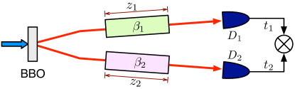
Figure 1: Each photon of the entangled photon pair is subject to different dispersion $\beta_{1}$ and $\beta_{2}$. The coincidence circuit measures $G^{(2)}(t_{1}-t_{2})$.

Let us first briefly discuss the theory behind nonlocal dispersion cancellation franson ; fitch . Consider a pair of spontaneous parametric down-conversion (SPDC) photons generated at a BBO crystal pumped by a monochromatic pump, see Fig. 1. The quantum state of the photon pair,

$$|\psi\rangle=\int d\omega_{1}d\omega_{2}\mathcal{S}(\omega_{1},\omega_{2})a^{\dagger}(\omega_{1})a^{\dagger}(\omega_{2})|0\rangle,$$ (1)

is an entangled state since the two-photon joint spectral amplitude $\mathcal{S}$ is non-factorizable, i.e., $\mathcal{S}(\omega_{1},\omega_{2})\neq\mathcal{S}(\omega_{1})\mathcal{S}(\omega_{2})$, due to the monochromatic nature of the pump kim05 ; baek08a . The joint detection probability of the two detectors $D_{1}$ and $D_{2}$ is proportional to the Glauber second-order correlation function

$$G^{(2)}(t_{1},t_{2})=|\langle 0|E_{2}^{(+)}(t_{2})E_{1}^{(+)}(t_{1})|\psi\rangle|^{2},$$ (2)

where $E_{1}^{(+)}(t_{1})=\int d\omega\,a(\omega_{1})e^{i\{k_{1}z_{1}-\omega_{1}t_{1}\}}$, the positive frequency part of the electric field operator at detector $D_{1}$, and $E_{2}^{(+)}$ is defined similarly. Since each photon has spectral distribution centered at certain central frequency, $\Omega_{1}$ and $\Omega_{2}$, and assuming that the photons propagate through dispersive media of length $z_{1}$ and $z_{2}$ as shown in Fig. 1, the wave number of the photon can then be expressed as $k_{i}(\Omega_{i}\pm\nu)=k_{i}(\Omega_{i})\pm\alpha_{i}\nu+\beta_{i}\nu^{2}$ ($i=1,2$). Here $\nu$ is the detuning frequency from the central frequency, and $\alpha$ and $\beta$ are the first-order and the second-order dispersion which are responsible for the wave packet delay and the wave packet broadening, respectively.

For a monochromatic pump, the quantum state in eq. (1) can be re-written as

$$|\psi\rangle=\int d\nu\mathcal{S}(\nu)a^{\dagger}(\Omega_{1}+\nu)a^{\dagger}(\Omega_{2}-\nu)|0\rangle,$$ (3)

with $\mathcal{S}(\nu)=\textrm{sinc}(\nu DL/2)$ for nondegenerate type-I SPDC. Here, $L$ and $D\equiv 1/u_{2}-1/u_{1}$ are the BBO crystal thickness and the inverse group velocity difference between the photon pair in the BBO crystal, respectively. Equation (2) can then be expressed as,

$$G^{(2)}(t_{1}-t_{2}) = \left|\int_{-\infty}^{\infty}d\nu\>\mathcal{S}(\nu)\>e^{i\nu(t_{1}-t_{2})}\right.\left.\times e^{i(\alpha_{1}z_{1}-\alpha_{2}z_{2})\nu}e^{i(\beta_{1}z_{1}+\beta_{2}z_{2})\nu^{2}}\right|^{2}.$$

The above expression can be analytically evaluated by approximating the joint spectral amplitude as a Gaussian function $\mathcal{S}(\nu)\approx e^{-\gamma(\nu DL)^{2}}$. The value $\gamma=0.04822$ was chosen so that the approximated Gaussian function would have the same full width at half maximum as the original function.

We, therefore, arrive at

$$G^{(2)}(t_{1}-t_{2})\approx Ce^{-(t_{1}-t_{2}-\bar{\tau})^{2}/2\sigma^{2}},$$ (4)

where $\bar{\tau}=\alpha_{2}z_{2}-\alpha_{1}z_{1}$ and $\sigma^{2}=\gamma D^{2}L^{2}+(\beta_{1}z_{1}+\beta_{2}z_{2})^{2}/\gamma D^{2}L^{2}$ are the overall time delay between the signal and the idler photons and the width of $G^{(2)}$ function after propagating through the dispersion media, respectively. Note that $C=\pi/\sqrt{\gamma^{2}D^{4}L^{4}+(\beta_{1}z_{1}+\beta_{2}z_{2})^{2}}$ is an unimportant proportionality factor.

Finally, the full width at half maximum value of the temporal width of $G^{(2)}$ function is given as note0

$$\Delta t\approx 2\sqrt{\frac{2\ln 2}{\gamma D^{2}L^{2}}}(\beta_{1}z_{1}+\beta_{2}z_{2}).$$ (5)

The above equation shows precisely the effect we have been looking for: a positive dispersion $\beta_{1}$ experienced by photon 1 can be cancelled by a negative dispersion $\beta_{2}$ experienced by photon 2. Such nonlocal dispersion cancellation effect is shown to occur only if photon 1 and photon 2 are in a specific entangled state franson .

III Experiment

The experimental setup to implement the nonlocal dispersion cancellation effect discussed above is schematically shown in Fig. 2. We first describe the entangled photon generation part of the experimental setup which is not shown in the figure. A 3 mm thick type-I $\beta$-barium borate (BBO) crystal is pumped by a cw diode laser operating at 408.2 nm (40 mW), generating a pair of collinear frequency-nondegenerate entangled photons centered at 896 nm and 750 nm via the SPDC process. Type-I collinear phase matching ensures that both the signal and idler photons of SPDC have very broad spectra centered at 896 nm (over 28 nm at FWHM) and 750 nm (over 20 nm at FWHM), respectively. The photon pair, however, is strongly quantum correlated in wavelength: if the signal photon is found to have the wavelength $\lambda_{1}$, then its conjugate idler photon will be found to have the wavelength $\lambda_{2}=\lambda_{p}\lambda_{1}/(\lambda_{1}-\lambda_{p})$, where $\lambda_{p}=408.2$ nm. The photon pair is in the two-photon quantum superposition (i.e., entangled) state of eq. (3).

To efficiently couple these photons into single-mode optical fibers, the pump laser was focused with a $f=300$ mm lens and the SPDC photons were coupled into single-mode optical fibers using $\times 10$ objective lenses located at 600 mm from the crystal. The pump beam waist at the focus is roughly 80 $\mu$m. The co-propagating photons were then separated spatially by using a beam splitter and two interference filters with 100 nm FWHM bandwidth, each centered at 896 nm and 750 nm. The 896 nm centered signal photon ($\lambda_{1}$ in Fig. 2) is then coupled into a 1.6 km long single-mode optical fiber which introduces positive dispersion $\beta_{1}$ to the photon. As we shall show later, the effect of a positive dispersion material to the entangled photon is to broaden the biphoton wave packet valencia ; baek08b ; baek08c .

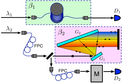
Figure 2: Schematic of the experiment. Positive dispersion $\beta_{1}$ is introduced by a 1.6 km long single-mode optical fiber and negative dispersion $\beta_{2}$ is introduced by using a pair of gratings ($G_{1}$ and $G_{2}$) and a mirror. FPC and M represent a fiber polarization controller and a monochromator, respectively.

To demonstrate the nonlocal dispersion cancellation effect, it is necessary to introduce negative dispersion to the idler photon ($\lambda_{2}$ in Fig. 2). Among many potential methods for introducing negative dispersion book , methods based on a grating pair or a prism pair are often used in ultrafast optics treacy ; fork . In our experiment, we have used the grating pair method to introduce negative dispersion to the idler photon.

The idler photon is first coupled into a 2 m long single-mode fiber and the fiber polarization controller (FPC) is used to set the polarization to maximize the diffraction efficiency. The grating pair $G_{1}$ and $G_{2}$ and a plane mirror is used to setup the negative dispersion device shown in Fig. 2 grating . The distance between the two gratings is set at 10 cm and the deviation angle at 750 nm is $8^{\circ}$. Since the grating $G_{2}$ is not big enough to cover the full bandwidth, the grating pair system slightly reduces the spectral bandwidth of the idler photon. After experiencing negative dispersion, the idler photon is coupled into a different 2 m long single-mode fiber for collimation and is sent through a 1/2 m monochromator (CVI DK480) which functions as a tunable narrowband filter. The monochromator M is used to spectrally-resolve the entangled biphoton wave packet baek08b ; baek08c .

Finally, the entangled biphoton wave packet is measured with two single-photon detectors and a time-correlated single-photon counting (TCSPC; PicoHarp 300, 16 ps resolution) device. The TCSPC histogram directly visualizes the second-order Glauber correlation function $G(t_{1}-t_{2})$, if the observed effects are sufficiently bigger than the resolution of the measurement system. The timing resolution of the measurement system was found to be 762 ps which corresponds to the width of the TCSPC histogram with the signal and the idler photons coupled into 4 m long single-mode optical fibers.

IV Results and Analysis

We first observed the entangled photon wave packet when the signal photon was passed through a 1.6 km single-mode optical fiber which introduces the positive dispersion $\beta_{1}$. The total length of the idler photon’s passage through the single-mode optical fiber is 4 m. Since we hope to observe the full TCSPC histogram which represents the dispersion broadened entangled photon wave packet, the monochromator M was not used for this measurement. The experimental data are shown in Fig. 3(a). The measured TCSPC histogram has the FWHM width of 3.861 ns which is significantly bigger than the timing resolution of the measurement system and is due to the dispersive broadening of the entangled photon wave packet.

To experimentally demonstrate the nonlocal dispersion cancellation effect, it is necessary to introduce negative dispersion $\beta_{2}$ to the idler photon so that the positive dispersion $\beta_{1}$ experienced by the signal photon is cancelled by the negative dispersion $\beta_{2}$ experienced by the idler photon franson ; fitch . The experiment was performed by directing the idler photon through the grating pair system for negative dispersion, while the signal photon’s passage through the 1.6 km single-mode fiber was not changed. As before, the monochromator M was not used for this measurement as we aim to observe the full TCSPC histogram.

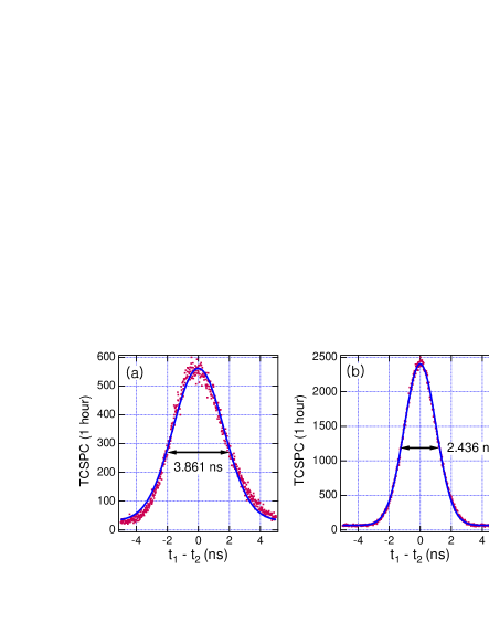
Figure 3: Experimentally measured entangled photon wave packet. Monochromator was not used for this measurement. (a) With positive dispersion $\beta_{1}$ only, the wave packet has the FWHM width of 3.861 ns. (b) With both positive dispersion $\beta_{1}$ and negative dispersion $\beta_{2}$, the wave acket has the FWHM width of 2.436 ns. Solid lines are Gaussian fit to the data.

The experimental data for this measurement are shown in Fig. 3(b). While the data clearly demonstrate reduced FWHM (2.436 ns) of the TCSPC histogram when compared to Fig. 3(a), Fig. 3 itself is quite insufficient for a conclusive demonstration of the nonlocal dispersion effect. It is because the grating pair system slightly reduces the spectral bandwidth of the idler photon and the reduced FWHM shown in Fig. 3(b) could be solely due to the bandwidth reduction.

It is thus critically important to attribute how much of the wave packet reduction observed in Fig. 3 has actually come from the nonlocal dispersion cancellation effect, if any. This critical measurement was accomplished by spectrally resolving the two entangled photon wave packets in Fig. 3 by introducing the monochromator M in the path of the idler photon baek08b ; baek08c . The monochromator was set to have roughly 1.2 nm of passband and it functions as a wavelength-variable bandpass filter. The TCSPC histograms measured for several values of the wavelength setting of the monochromator correspond to spectrally resolved components of the entangled photon wave packets shown in Fig. 3.

Observation of nonlocal dispersion cancellation then requires comparing the temporal spacing between the spectrally resolved components of the entangled photon wave packets. If the temporal spacing between the spectrally resolved components are reduced by the introduction of the grating pair, it conclusively confirm the nonlocal dispersion cancellation effect in Ref. franson ; fitch . On the other hand, if the temporal separation remains the same while some of the components showing reduced amplitudes, it would mean that the overall wave packet reduction is actually due to the bandwidth filtering.

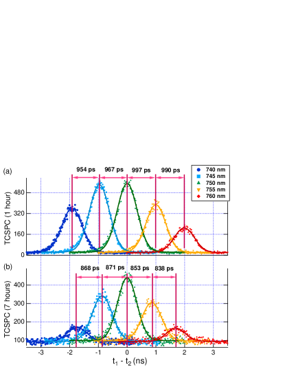
Figure 4: Spectrally-resolved entangled photon wave packet with the monochromator. (a) With positive dispersion $\beta_{1}$ only. (b) With both positive dispersion $\beta_{1}$ and negative dispersion $\beta_{2}$. Solid lines are Gaussian fit to the data. The nonlocal dispersion cancellation effect is clear demonstrated.

The experimental data are shown in Fig. 4. In Fig. 4(a), the entangled photon wave packet with positive dispersion $\beta_{1}$ introduced in the path of the signal photon is spectrally resolved. In Fig. 4(b), we show the spectrally resolved entangled photon wave packet when both $\beta_{1}$ and $\beta_{2}$ are introduced. Comparing Fig. 4(a) and Fig. 4(b), we observe that the temporal spacings between the spectrally resolved components are reduced when the idler photon is subject to negative dispersion $\beta_{2}$. This is a clear and conclusive signature of the nonlocal dispersion cancellation effect. It is also interesting to observe that certain spectral components (most notably, 740 nm and 760 nm) are strongly attenuated, causing reduction of the entangled photon wave packet.

The above observations allow us to conclude that the reduced entangled photon wave packet in Fig. 3(b) is due to both the nonlocal dispersion cancellation effect and the bandwidth reduction by the grating pair system. The experimental data in Fig. 4 show that the reduction of the temporal spacing between 740 nm and 760 nm is 478 ps. To see what the theoretically expected value is, we need to make use of eq. (5). The introduction of $\beta_{2}$ reduces the width of $G^{(2)}$ function by

$$\Delta t_{\textrm{NDC}}\approx 2\sqrt{\frac{2\ln 2}{\gamma D^{2}L^{2}}}\beta_{2}z_{2}.$$

In our experiment, $DL=88.9$ fs and $\beta_{2}z_{2}$ for the grating pair system is given as diels ,

$$\beta_{2}z_{2}=-\frac{\lambda_{2}}{2\pi c^{2}}\left(\frac{\lambda_{2}}{d}\right)\frac{G}{\cos(\theta^{\prime})^{3}},$$

where $c$ is the vacuum speed of light, $\lambda_{2}=750$ nm, $d=1/2400$ mm, $G=10$ cm, and $\theta^{\prime}=60.45^{\circ}$. From these values, we obtain $\beta_{2}z_{2}=-(2.03\textrm{ ps})^{2}$. The theoretically calculated value of the reduction of the biphoton wave packet, therefore, is approximately 496 ps. Considering the measurement errors for evaluating $\beta_{2}z_{2}$, our experimental observation agrees very well with the theoretical prediction.

We therefore estimate that, out of 1.425 ns reduction of the wave packet shown in Fig. 3, roughly 478 ps comes from the nonlocal dispersion cancellation effect and the rest comes from the bandwidth filtering at the grating pair. To improve the nonlocal dispersion cancellation effect, it is necessary to eliminate the bandwidth reduction effect of the grating pair system and it can be done by replacing the grating $G_{2}$ with a larger one.

V Discussion

Using the spontaneous parametric down-conversion photon pairs whose central frequencies are anticorrelated as in eq. (3), we have shown that two-photon entanglement (i.e., the coherent superposition of frequency-anticorrelated biphoton amplitudes) can exhibit the nonlocal dispersion cancellation effect, see eq. (5) franson . Naturally, one might wonder whether some classical frequency-anticorrelated states could also exhibit the nonlocal dispersion cancellation effect. In this section, we discuss these classical cases and show that it is not possible to achieve the nonlocal dispersion cancellation effect of Ref. franson using classical states.

V.1 A frequency-anticorrelated mixture of two-photon states

Spontaneous parametric down-conversion produces a two-photon pure state as shown in eq. (3). Let us see what would happen if phase coherence is removed so that the input state is now a frequency-anticorrelated mixture of two-photon states given as

$$\rho_{mixed} = \int d\nu f_{1}(\nu)f_{2}(\nu)a^{\dagger}(\Omega_{1}+\nu)a^{\dagger}(\Omega_{2}-\nu)|0\rangle\langle 0|$$ (6)

$$a(\Omega_{1}+\nu)a(\Omega_{2}-\nu),$$

where $f_{1}(\nu)=f_{2}(\nu)=e^{-\nu^{2}/2\sigma^{2}}$ are spectral amplitudes of photon 1 and photon 2 and we assume they follow gaussian spectral distribution. The normalization condition gives $\int d\nu f_{1}(\nu)f_{2}(\nu)=1$. Such states might experimentally be approximated by using a pair of strongly attenuated cw lasers whose frequencies are tuned in opposite directions by the random amount $\nu$ and filtered by Gaussian filters with transmission function $f_{1}(\nu)$ and $f_{2}(\nu)$.

When $\rho_{mixed}$ is used in the experimental setup shown in Fig. 1, the joint detection rate between two detectors $D_{1}$ and $D_{2}$ is proportional to the Glauber 2nd-order correlation function

$$G^{(2)}(t_{1},t_{2})=Tr[\rho_{mixed}E_{1}^{(-)}(t_{1})E_{2}^{(-)}(t_{2})E_{2}^{(+)}(t_{2})E_{1}^{(+)}(t_{1})],$$ (7)

where $E_{1}^{(+)}(t_{1})=\int d\nu a(\nu)e^{i\{k_{1}z_{1}-(\Omega_{1}+\nu)t_{1}\}}$, the positive frequency component of the electric field operator at detector $D_{1}$, and $E_{2}^{(+)}$ is defined similarly. By combining eq. (6) and eq. (7), we finally obtain

$$G^{(2)}(t_{1},t_{2})=1.$$ (8)

Physically, this means that the joint detection probabilities of two detectors do not depend on time at all. In other words, even $D_{1}$ detects a photon at $t_{1}$, we have no information about when $D_{2}$ would click. The joint detection probability does not show timing information at all and, therefore, is meaningless to discuss the dispersive effect with the two-photon mixed state. This result tells us that coherence between two-photon probability amplitudes (i.e., entanglement) is essential for the nonlocal dispersion cancellation effect.

V.2 A classical pulse pair

Let us now consider whether the nonlocal dispersion cancellation effect of Ref. franson can be exhibited by a classical pulse pair. First, assume two ultrafast pulses which are initially coincident in time franson . The frequency of each pulse can be defined as $\omega_{1}=\Omega_{1}+\nu_{1}$ and $\omega_{2}=\Omega_{2}-\nu_{2}$, respectively. Here $\nu_{i}$ is the detuning frequency from the central frequency $\Omega_{i}$ and the subscript $i$ labels each pulse ($i=1,2$). The wave number of the photon can then be expressed as $k_{i}(\Omega_{i}\pm\nu_{i})\thickapprox k_{i}(\Omega_{i})\pm\alpha_{i}\nu_{i}+\beta_{i}\nu_{i}^{2}$. Note that $\alpha$ and $\beta$ are the first-order and the second-order dispersion which are responsible for the wave packet delay and the wave packet broadening, respectively.

After pulse 1 has propagated through the dispersive medium $\beta_{1}$, see Fig. 1, the electric field at the detector can then be written as

$$E_{1}(t_{1},z_{1}) = \int_{-\infty}^{\infty}d\nu_{1}\frac{E_{0}}{2\pi}e^{-\nu_{1}^{2}/2\sigma_{0}^{2}}e^{i(k_{1}(\Omega_{1})+\alpha_{1}\nu_{1}+\beta_{1}\nu_{1}^{2})z_{1}}$$ (9)

$$\times e^{-i(\Omega_{1}+\nu_{1})t_{1}},$$

where $E_{0}$ is a constant, $\sigma_{0}$ is the bandwidth of the pulse, $z_{1}$ is the distance between the light source and the detector, and $t_{1}$ is the detection time. $E_{2}(t_{2},z_{2})$ for pulse 2 is defined similarly.

The intensity detected at $D_{1}$ is $I_{1}(z_{1},t_{1})=|E_{1}(z_{1},t_{1})|^{2}$ and is calculated to be

$$I_{1}(z_{1},t_{1})=\frac{E_{0}^{2}}{4\pi|a_{1}|^{2}}e^{-(\alpha_{1}z_{1}-t_{1})^{2}/2\sigma_{1}^{2}},$$ (10)

where $a_{1}^{2}=1/2\sigma_{0}^{2}-i\beta_{1}z_{1}$ and $\sigma_{1}^{2}=2\sigma_{0}^{2}(1/4\sigma_{0}^{4}+\beta_{1}^{2}z_{1}^{2})$. The intensity at $D_{2}$ is calculated similarly as

$$I_{2}(z_{2},t_{2})=\frac{E_{0}^{2}}{4\pi|a_{2}|^{2}}e^{-(\alpha_{2}z_{2}-t_{2})^{2}/2\sigma_{2}^{2}},$$ (11)

where $a_{2}^{2}=1/2\sigma_{0}^{2}-i\beta_{2}z_{2}$ and $\sigma_{2}^{2}=2\sigma_{0}^{2}(1/4\sigma_{0}^{4}+\beta_{2}^{2}z_{2}^{2})$.

The joint detection probability, i.e., the probability that two detectors $D_{1}$ and $D_{2}$ click simultaneously at times $t_{1}$ and $t_{2}=t_{1}+\tau$ is then given as $\eta I_{1}(z_{1},t_{1})I_{2}(z_{2},t_{1}+\tau)$, where $\eta$ is a constant related to the detection efficiency, and is calculated to be

$$P(\tau)=\int_{-\infty}^{\infty}dt_{1}\eta I_{1}(z_{1},t_{1})I_{2}(z_{2},t_{1}+\tau)=Ce^{-\frac{(\tau-\overline{\tau})^{2}}{2(\sigma_{1}^{2}+\sigma_{2}^{2})}},$$ (12)

where $\overline{\tau}=\alpha_{2}z_{2}-\alpha_{1}z_{1}$ and $C=\eta E_{0}^{4}/[(4\pi)^{2}|a_{1}|^{2}|a_{2}|^{2}]\int_{-\infty}^{\infty}\exp[-\frac{1}{2}(\frac{1}{\sigma_{1}^{2}}+\frac{1}{\sigma_{2}^{2}})t_{1}^{2}]dt_{1}$.

The joint detection or the coincidence distribution $P(\tau)$ then has a total width

$$\sigma_{T}^{2}=\sigma_{1}^{2}+\sigma_{2}^{2}=2\sigma_{0}^{2}(1/2\sigma_{0}^{4}+\beta_{1}^{2}z_{1}^{2}+\beta_{2}^{2}z_{2}^{2}),$$ (13)

and for large distances and dispersions, eq. (13) becomes

$$\sigma_{T}^{2}\approx 2\sigma_{0}^{2}(\beta_{1}^{2}z_{1}^{2}+\beta_{2}^{2}z_{2}^{2}).$$ (14)

Finally, the full width at half maximum value of the temporal width of $P(\tau)$ is given as

$$\Delta t\approx 4\sqrt{\ln 2}\sigma_{0}\sqrt{\beta_{1}^{2}z_{1}^{2}+\beta_{2}^{2}z_{2}^{2}}.$$ (15)

Since eq. (15) depends on the summation of squares of individual dispersion values, nonlocal dispersion cancellation is not possible using two classical pulses even in the case $\beta_{1}=-\beta_{2}$. Clearly, this is due to the local nature of classical fields franson . Even if the two classical pulses are anticorrelated in their central frequencies, the rest of frequency components of pulse 1 and pulse 2 do not have spectral nor temporal correlations. As a result, the local dispersion experienced by pulse 1 cannot be canceled by the local dispersion experienced by pulse 2.

The effect of dispersion on the joint detection probability of the classical pulse pair can be easily described using Fig. 5(a). The detection probability as a function of time for a short pulse (pulse 1) after it has propagated through a positive dispersion medium $+\beta$ is given as $P_{1}(t_{1})$. The detection probability for pulse 2 after it has propagated through a negative dispersion medium $-\beta$ is given as $P_{2}(t_{2})$. $P_{1}(t_{1})$ and $P_{2}(t_{2})$ show the wave packet broadening due to eq. (10) and eq. (11), respectively. The result in eq. (15) shows that the joint detection probability $P_{c}(t_{1}-t_{2})$ would then be much broader than $P_{1}(t_{1})$ and $P_{2}(t_{2})$ individually as depicted in Fig. 5(a). Note that this case is referred in Fig. 5(a) as ($+\beta$,$-\beta$). Exactly the same results are obtained for other cases, namely, ($+\beta$, $+\beta$), ($-\beta$, $+\beta$), and ($-\beta$,$-\beta$).

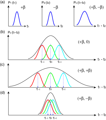
Figure 5: The joint detection probability for a number of cases involving classical pulse pairs under group velocity dispersion. (a) Detection probabilities for pulse 1, $P_{1}(t_{1})$, and pulse 2, $P_{2}(t_{2})$, after they have propagated through $+\beta$ and $-\beta$ media, respectively. The joint detection probability $P_{c}(t_{1}-t_{2})$ is always broader then the single detection probabilities. Note that ($+\beta$,$-\beta$) refers to the case in which pulse 1 (pulse 2) goes through the positive (the negative) dispersive medium. Figures (b), (c), and (d) show the joint detection probabilities for a frequency-anticorrelated mixture of classical pulse pairs. Note that ($+\beta$,$0$) refers to the case in which pulse 1 goes through the positive dispersion medium while pulse 2 goes through a non-dispersive medium. ($+\beta$,$+\beta$), and ($+\beta$,$-\beta$) have similar meanings. If spectrally identical sources are used, the the overall joint detection probabilities cannot be smaller than the individual probabilities. See text for details.

V.3 A frequency-anticorrelated mixture of classical pulse pairs

Let us now consider a frequency-anticorrelated mixture of classical pulse pairs. Here we imagine many frequency-anticorrelated pulse pairs, each with a random amount of detuning $\nu$ from the central frequency $\Omega$. Thus, a pulse pair is always frequency-anticorrelated but no pairs have the same amount of detuning. We also assume a sufficiently broadband Gaussian filters are placed in front of the detectors.

Clearly, the joint detection probability for each pulse pair is described by eq. (15). However, since each pulse pair has different central frequencies than the previous/next ones, the coincidence peak for each pulse pair, after they have propagated through the dispersion media, would then appear at different times due to the dispersion.

The coincidence peak corresponding to the $m$’th pulse pair occurs at

$$\tau_{m}=\frac{z_{1}}{v_{1}(\Omega+m\nu)}-\frac{z_{2}}{v_{2}(\Omega-m\nu)},$$ (16)

where $m$ is an integer, $v_{i}$ is the group velocity of pulse $i$ ($i=1,2$), and $z_{i}$ is the distance between the source and the detector. Note that $\tau_{m}$, the time at which the coincidence peak corresponding to the $m$’th pulse pair occurs, is simply the relative group delay between the two pulses. In what follows, we will explore how the statistical distribution of $\tau_{m}$ is affected by the dispersive media.

CASE I ($+\beta$, 0): Consider the case that pulse 1 is sent to a positive dispersive medium, $+\beta$, and pulse 2 is sent to a nondispersive medium (e.g., air). In this case, the group velocity of pulse 2 can be approximated as $v_{2}(\Omega-m\nu)\approx c$, where $c$ is the speed of light in the air, and eq. (16) can be rewritten as $\tau_{m}=z_{1}/v_{1}(\Omega+m\nu)-z_{2}/c$. When the cental frequency of pulse 1 is tuned to $\Omega\pm\nu$ ($\nu>0$) from $\Omega$, the coincidence peak is shifted from $\tau_{0}=z_{1}/v_{1}(\Omega)-z_{2}/c$ to $\tau_{\pm 1}=z_{1}/v_{1}(\Omega\pm\nu)-z_{2}/c$. Since the group delay of pulse 1 monotonously increases as the frequency increases for the positive dispersion medium, the group delays corresponding to the three coincidence peaks satisfy the relation, $\tau_{-1}<\tau_{0}<\tau_{+1}$, as shown in Fig. 5 (b).

We can then define the measure of the width of the coincidence distribution as

$$\Delta\tau(+\beta,0)\equiv\tau_{+1}-\tau_{0}=\frac{z_{1}}{v_{1}(\Omega+\nu)}-\frac{z_{1}}{v_{1}(\Omega)}.$$ (17)

When the coincidence measurement is done for a sufficiently long time, it will take the form of a broadened Gaussian envelope (due to the Gaussian filters) as shown in Fig. 5(b).

CASE II ($+\beta$, $+\beta$): Let us now consider the case that pulse 1 and pulse 2 are both sent to positive dispersion media. Considering that the pulse pair is frequency-anticorrelated in their central frequencies and the dispersion is positive for both pulses, the relative group delays can be calculated using eq. (16) as $\tau_{0}=z_{1}/v_{1}(\Omega)-z_{2}/v_{2}(\Omega)$ and $\tau_{+1}=z_{1}/v_{1}(\Omega+\nu)-z_{2}/v_{2}(\Omega-\nu)$. The coincidence width is then calculated to be

$$\Delta\tau(+\beta,+\beta)=\tau_{+1}-\tau_{0}=\Delta\tau(+\beta,0)+\frac{z_{2}}{v_{2}(\Omega)}-\frac{z_{2}}{v_{2}(\Omega-\nu)},$$ (18)

where $\Delta\tau(+\beta,0)$ is defined in eq. (17). Since pulse 2 propagates through the positive dispersion medium, $v_{2}(\Omega)<v_{2}(\Omega-\nu)$ and, therefore, $\Delta\tau(+\beta,+\beta)>\Delta\tau(+\beta,0)$. This case, shown in Fig. 5(c), therefore gives broader coincidence distribution than the $(+\beta,0)$ case shown in Fig. 5(b).

CASE III ($+\beta$, $-\beta$): Finally we discuss the case in which pulse 1 propagates through the positive dispersion medium while pulse 2 propagates through the negative dispersion medium. Remember that the pulse pair mixture is frequency-anticorrelated and each pair has random detuning. Since pulse 2 propagates through the negative dispersion medium, $v_{2}(\Omega)>v_{2}(\Omega-\nu)$ and, therefore, $\Delta\tau(+\beta,-\beta)=\tau_{+1}-\tau_{0}=\Delta\tau(+\beta,0)+z_{2}/v_{2}(\Omega)-z_{2}/v_{2}(\Omega-\nu)<\Delta\tau(+\beta,0)$. As a result, the relative group delay $\tau_{m}$ does not increase much from the $\tau_{0}$ value even with large $m$’s. The coincidence peak, therefore, occurs mostly at around $\tau_{0}=z_{1}/v_{g}(\Omega)-z_{2}/v_{g}(\Omega)$ as shown in Fig. 5(d).

Thus, for the frequency-anticorrelated mixture of classical pulse pairs, we arrive at the relation,

$$\Delta\tau(+\beta,+\beta)>\Delta\tau(+\beta,0)>\Delta\tau(+\beta,-\beta).$$ (19)

One might try to interpret the above result as showing, even with the frequency-anticorrelated mixture of classical pulse pairs, it is possible to achieve the nonlocal dispersion cancellation effect. This, however, is an erroneous conclusion because the minimum coincidence distribution in time is limited by eq. (15), depicted in Fig. 5(a), which is quite different from the quantum nonlocal dispersion cancellation effect in eq. (5).

VI Conclusion

We have reported an experimental demonstration of the quantum nonlocal dispersion cancellation effect of Ref. franson in which the signal photon is subject to positive dispersion while its entangled twin photon, remotely located, is subject to negative dispersion. In this work, for the first time, we have explicitly demonstrated the narrowing of the joint detection probability function by spectrally resolving the dispersion-broadened two-photon wave packet and the amount of narrowing has shown to be consistent with the theoretical calculations based on the quantum nonlocal dispersion cancellation effect. We have also shown theoretically that classical states, e.g., a two-photon mixed state and a frequency-anticorrelated mixture of classical pulse pairs, cannot demonstrate the nonlocal dispersion cancellation effect. We expect that the nonlocal dispersion cancellation effect will play an important role in fiber-based quantum communication and quantum metrology applications as the method to remotely remove/compensate unwanted dispersive effects on nonclassical wave packets.

References

- (1) J.D. Franson, Phys. Rev. A45, 3126 (1992).
- (2) C.K. Hong, Z.Y. Ou, and L. Mandel, Phys. Rev. Lett. 59, 2044 (1987).
- (3) Y.-H. Kim, S.P. Kulik, and Y. Shih, Phys. Rev. Lett 86, 1370 (2001).
- (4) P.P. Rohde and T.C. Ralph, Phys. Rev. A72, 052332 (2005).
- (5) T. Jennewein, R. Ursin, M. Aspelmeyer, and A. Zeilinger, J. Phys. B: At. Mol. Opt. Phys. 42, 114008 (2009).
- (6) V. Giovannetti, S. Lloyd, L. Maccone, and F. N. C. Wong, Phys. Rev. Lett. 87, 117902 (2001).
- (7) V. Giovannetti, S. Lloyd, and L. Maccone, Nature (London) 412, 417 (2001).
- (8) M.J. Fitch and J.D. Franson, Phys. Rev. A65, 053809 (2002).
- (9) J. Brendel, H. Zbinden, N. Gisin, Opt. Communications 151, 35 (1998).
- (10) The demonstration in Ref. gis is local in the sense that both photons propagate through the same optical fiber. Furthermore, actual reduction of a broadened wave packet is not experimentally demonstrated.
- (11) A.M. Steinberg, P.G. Kwiat, and R.Y. Chiao, Phys. Rev. Lett. 68, 2421 (1992).
- (12) M.B. Nasr, B.E.A. Saleh, A.V. Sergienko, and M.C. Teich, Phys. Rev. Lett. 91, 083601 (2003).
- (13) Dispersion cancellation of Ref. steinberg ; nasr is based on Hong-Ou-Mandel interference, which is a first order correlation effect, , related only to the power spectrum of the field, just as classical Michelson interference kim03 . It, therefore, is not a nonlocal effect and there exists a classical analog. On the other hand, nonlocal dispersion cancellation of Ref. franson is a genuine second order correlation effect, ; the dispersion experienced by one photon is nonlocally cancelled by the dispersion experienced by it’s entangled pair photon which may be arbitrarily far apart. See Ref. franson08 .
- (14) J.D. Franson, prreprint arXiv: 0907.5196 (2009).
- (15) Y.-H. Kim, J. Opt. Soc. Am. B. 20, 1959 (2003).
- (16) J.D. Franson, Proceedings of the 9th Rochester Conference on Coherence and Quantum Optics, eds. N.P. Bigelow, J.H. Eberly, and C.R. Stroud, “Nonlocal Interferometry: Beyond Bell’s Inequality,” Jr. (American Institute of Physics, 2008).
- (17) Y.-H. Kim and W.P. Grice, Opt. Lett. 30, 908 (2005).
- (18) S.-Y. Baek and Y.-H. Kim, Phys. Rev. A77, 043807 (2008).
- (19) We have assumed . This condition holds in general as the crystal parameter is much smaller than the external parameters and .
- (20) A. Valencia, M.V. Chekhova, A. Trifonov, and Y. Shih, Phys. Rev. Lett. 88, 183601 (2002).
- (21) S.-Y. Baek, O. Kwon, and Y.-H. Kim, Phys. Rev. A77, 013829 (2008).
- (22) S.-Y. Baek, O. Kwon, and Y.-H. Kim, Phys. Rev. A78, 013816 (2008).
- (23) B.E.A. Saleh and M.C. Teich, Fundamentals of Photonics, (Wiley & Sons, Hoboken, New Jersey, 2007).
- (24) E.B. Treacy, IEEE J. Quantum Electron. QE-5, 454 (1969).
- (25) R.L. Fork, O.E. Martinez, J.P. Gordon, Opt. Lett. 9, 150 (1984).
- (26) The grating and are Spectrogon 715.701.990 and 715.701.350, respectively. The grating specifications can be found at http://www.spectrogon.com/gratpulse.html.
- (27) J.-C. Diels and W. Rudolph, Ultrashort Laser Pulse Phenomena (Academic Press, Burlington, MA, 2006).
- (28) K.J. Resch, P. Puvanathasan, J.S. Lundeen, M.W. Mitchell, and K. Bizheva, Optics Express 15, 8797 (2007).