The phase diagram of the extended anisotropic ferromagnetic-antiferromagnetic Heisenberg chain

Abstract

By using Density Matrix Renormalization Group (DMRG) technique we study the phase diagram of 1D extended anisotropic Heisenberg model with ferromagnetic nearest-neighbor and antiferromagnetic next-nearest-neighbor interactions. We analyze the static correlation functions for the spin operators both in- and out-of-plane and classify the zero-temperature phases by the range of their correlations. On clusters of $64,100,200,300$ sites with open boundary conditions we isolate the boundary effects and make finite-size scaling of our results. Apart from the ferromagnetic phase, we identify two gapless spin-fluid phases and two ones with massive excitations. Based on our phase diagram and on estimates for the coupling constants known from literature, we classify the ground states of several edge-sharing materials.

1 Introduction

Recently, an increasing attention has been paid to the materials containing edge-sharing ${\rm CuO_{2}}$ chains (e.g.
${\rm Rb_{2}Cu_{2}Mo_{3}O_{12}}$ as in Ref. hase , ${\rm NaCu_{2}O_{2}}$ as in Ref. drechsler_01 or ${\rm LiCuVO_{4}}$ as in Ref. enderle_00 ). It has been found by using several complementary experimental techniques that the low-energy physics in such materials is one-dimensional enderle_00 . It has been also concluded that in such insulating materials the spins, localized on the copper ions, interact via ferromagnetic interaction with their nearest neighbors, while a considerable next-nearest neighbor (NNN) interaction has been argued to be antiferromagnetic. In addition, at least in one material (${\rm LiCuVO_{4}}$), about 6$\%$ exchange anisotropy has been measured by using paramagnetic resonance nidda_00 ; vasiliev_00 . Another manifestation of such anisotropy is the dependence of the saturation value of the external magnetic field on its direction enderle_00 .

It is widely accepted that to study such systems, a 1D extended anisotropic Heisenberg model with ferromagnetic (F) nearest-neighbor (NN) interaction and antiferromagnetic (AF) NNN one should be used. In order to estimate the values of the exchange interactions in these materials, temperature and magnetic field dependencies of the integrated quantities, such as susceptibility and magnetization, have been compared with those of various 1D spin models, calculated exactly on small clusters. The F-AF Heisenberg model appeared to be the only compatible drechsler_01 . Excluding the symmetry breaking in $XY$-plane, the resulting Hamiltonian could have at most four parameters: two in-plane interaction constants and two out-of-plane ones. Let us denote these as follows $J_{\perp}$, $J^{\prime}_{\perp}$, $J_{z}$ and $J^{\prime}_{z}$. Since one of them can always be used to set the unit of energy, there are in fact only three independent interaction constants. Such large number of parameters makes it difficult to explore the full phase diagram, which would be three-dimensional. There exist several parametrizations of this system, which use less parameters. For instance, one can restrict oneself only to isotropic case ($J_{z}=J_{\perp}$, $J^{\prime}_{z}=J^{\prime}_{\perp}$), ending up with only one parameter i.e. $J_{z}/J_{z}^{\prime}$, and two cases, according to the sign of $J_{z}^{\prime}$, as in the Ref. tonegawa . Contrarily, one could allow for the same level of anisotropy both in NN and NNN channels, which results in two parameters i.e. $J_{z}=\pm 1$, $J^{\prime}_{z}/J_{z}$ and $J_{\perp}/J_{z}\equiv J^{\prime}_{\perp}/J^{\prime}_{z}$, as in the Ref. hirata . Yet, another parametrization, adopted in the present paper, consists in letting the anisotropy only in the NN channel, while leaving the NNN interaction isotropic, as in Ref. haldane_03 . This parametrization amounts to have two parameters: $J_{z}=\pm 1$, $J_{\perp}/J_{z}$ and $J^{\prime}/J_{z}\equiv J^{\prime}_{z}/J_{z}=J^{\prime}_{\perp}/J_{z}$. Accordingly, the 1D extended anisotropic Heisenberg model reads as follows (contrarily to Ref. haldane_03 we invert the sign of $J_{z}$):

$$H = -J_{z}\sum_{i}S^{z}_{i}S^{z}_{i+1}+J_{\bot}\sum_{i}(S^{x}_{i}S^{x}_{i+1}+S^{y}_{i}S^{y}_{i+1})$$ (1)

$$+ J^{\prime}\sum_{i}\mathbf{S}_{i}\mathbf{S}_{i+2}.$$

It is worth noting that the Hamiltonian (1) with $J_{\perp}>0$ can be easily mapped onto the one with $J_{\perp}<0$. Indeed, for a bipartite lattice, the transformation:

$$\tilde{S}^{\alpha}_{i}=(-1)^{i}S^{\alpha}_{i},\;\mathrm{where}\;\alpha=x,y.$$ (2)

inverts the sign in front of $J_{\perp}$ and changes an in-plane correlation function $\langle S^{\alpha}_{i}S^{\alpha}_{i+n}\rangle$ by the pre-factor $(-1)^{n}$. We choose AF sign of $J_{\perp}$ to be compatible with our previous work Plekhanov_01 , although in the edge-sharing ${\rm CuO_{2}}$ materials $J_{\perp}$ should be negative. While in edge-sharing materials the anisotropy has been found at least in one compound nidda_00 ; vasiliev_00 , its precise structure and strength is still difficult to estimate. In this article, we intend to study the qualitative effects of anisotropy and do not want to increase excessively the number of parameters. That is why we consider the anisotropy only in NN channel. Finally, it is worth noting that the model (1) can be also represented as a two-leg zigzag ladder as show in Fig. 1.

From the theoretical point of view, F-AF Heisenberg model is a challenge both for analytical and numerical methods. The model (1) has been extensively studied in its antiferromagnetic region white_03 ($J_{z}<0$). For what concerns the ferromagnetic region ($J_{z}>0$), a few results should be mentioned. First of all, it is worth noting that despite the non-integrability of the model, there exist two points in its parameter space where the analytic expression for the ground state energy and wave functions are known. These are the points: ($J_{z}=-1$, $J_{\perp}=J_{z}$, $J^{\prime}=J_{z}/2$) as proven in Ref. majumdar and ($J_{z}=1$, $J_{\perp}=J_{z}$, $J^{\prime}=J_{z}/4$) as found in Ref. hamada . Secondly, the famous Haldane conjecture haldane_01 ; haldane_02 states that one-dimensional AF NN spin chains, composed of half-integer spins, could only have massless excitations and power-law-decaying correlation functions. Another conjecture – the so-called “ladder conjecture” – comes from numerical methods dagotto ; hung , bosonization affleck_01 ; schultz and subsequently from experiments on a series of ladder materials like Sr_(n-1)/2Cu_(n+1)/2O_n $(n=3,5\ldots)$ azuma ; kojima . This conjecture states: “spin-$\frac{1}{2}$ ladders composed of an even number of chains have gapped excitations, while those with an odd number of chains have gapless excitations”. However, none of these arguments carries over to the extended anisotropic Heisenberg model (1) and therefore the issue of whether it could possess a gapped ground state and whether the gap can be observed numerically is still controversial. The existence of an astronomically small gap itoi (with a correlation length of the order of $10^{36}$ lattice spacings) has been predicted by means of the Renormalization Group analysis of the effective field theory in the limit of two AF chains coupled by a weak F inter-chain coupling. A gapped dimer phase, surrounded by the gapless spin-fluid ones, has also been identified by using the level-crossing analysis of the excited states obtained by Lanczos diagonalization on small rings nomura ; somma_01 . Similar results were found by using the Quantum Renormalization Group jafari . In addition, a dimerized gapped phase bursill , incommensurate power-law correlations nersesyan and chiral order kaburagi_00 ; kaburagi_01 ; kaburagi_02 have been found on the AF side of the model ($J_{z}<0$). On the other hand, in Ref.dmitriev_01 by means of the perturbation theory around the critical point ($J^{\prime}=0.25J_{z}$, $J_{\perp}=J_{z}$) of weakly anisotropic F-AF Heisenberg model, only spin-fluid gapless phases have been found. This result might be an artefact of the perturbation theory, since a perturbation can not change the underlying mean-field ground state unless one is summing up an infinite number of diagrams. Finite magnetic field phase diagram of the model (1) has been studied in the Refs. hm_00 ; hm_01 ; hm_02 ; sudan_00 , which gave an insight into the nature of elementary excitations unveiling both gapped and gapless excitations depending on the values of Hamiltonian parameters.

Figure 1: Mapping of the model (1) on a two-leg zigzag ladder.

Even for the NN Heisenberg model ($J^{\prime}=0$), despite the existence of exact Bethe-ansatz solution, it is still extremely difficult to obtain closed analytic expressions for the correlation functions (see e.g. kitanine_01 ; kitanine_02 ). Asymptotic analytical results come mainly from the Quantum Field Theory. In Ref. affleck it has been shown, based on the Conformal Field Theory, that the long-range behavior ($r\to\infty$) for the isotropic antiferromagnetic Heisenberg model has a highly non-trivial form:

$$\langle S^{\alpha}_{0}S^{\beta}_{r}\rangle\to\delta_{\alpha,\beta}\frac{(-1)^{r}}{(2\pi)^{3/2}}\frac{\sqrt{(\ln r)}}{r},$$ (3)

where $\alpha$, $\beta=x,y,z$. As soon as the rotational invariance is broken, however, the correlation functions of the nearest-neighbors anisotropic Heisenberg (XXZ) model assume a simple power-law form:

$$\langle S^{x}_{0}S^{x}_{r}\rangle \to (-1)^{r}A_{x}r^{\eta}+B_{x}r^{\eta+1/\eta}$$ (4)

$$\langle S^{z}_{0}S^{z}_{r}\rangle \to (-1)^{r}A_{z}r^{1/\eta}+B_{z}r^{-2}.$$ (5)

Here $\langle S^{y}_{0}S^{y}_{r\phantom{0}}\rangle=\langle S^{x}_{0}S^{x}_{r}\rangle$, $\eta=-\arccos(J_{z}/J_{\perp})/\pi$, $0\leq|J_{z}/J_{\perp}|<1$, $A_{x}$ has been determined in Ref. lukyanov and $A_{z},B_{x},B_{z}$ are not known in general for arbitrary values of the ratio $J_{z}/J_{\perp}$.

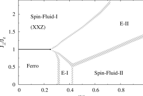
Figure 2: Quantum phase diagram of the Hamiltonian (1) (right panel) as compared to the classical one (left panel). The dashed regions are the phase boundaries determined with systematic error owing to the finiteness of the cluster size.

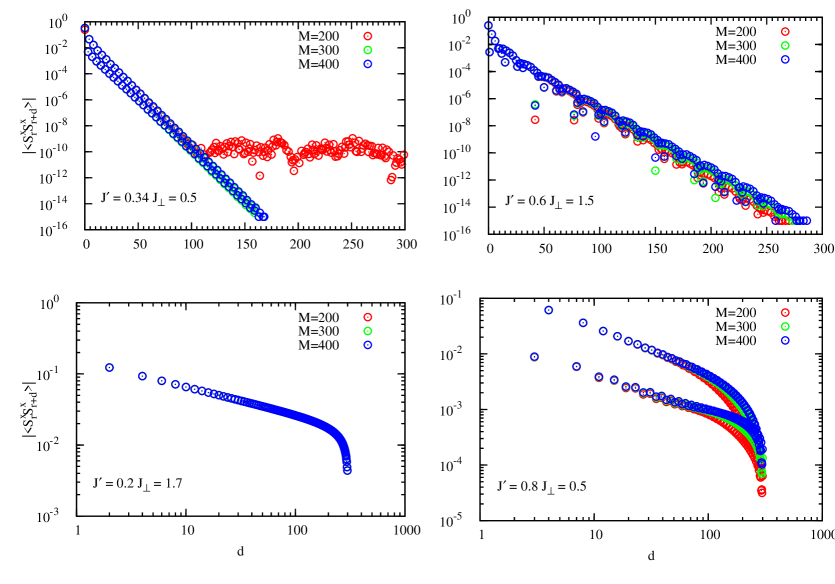
Figure 3: A study of DMRG truncation error as a function of the number of retained density matrix eigenstates $M$ at four points representing the phases E-I(top-left panel), E-II(top-right), Spin-Fluid-I(bottom-left), Spin-Fluid-II(bottom-right). In-plane correlation function is taken as an example.

In the past we have already considered the ferromagnetic ($J_{z}>0$) model (1) in connection with the question of ergodicity of the system’s dynamics Plekhanov_01 ; Plekhanov_02 , by means of the Lanczos and Exact Diagonalization techniques. Therein a zero-temperature phase diagram has been constructed, based on whether the dynamics of the $z$-projection of local spin was ergodic or not. Different types of ergodic phases have been identified depending on how the non-ergodic constant was approaching zero within the finite-size scaling. Another insight into the physics of (1) has been made from the entanglement studies of the phase transitions in the vicinity of the ferromagnetic phase. Two different types of behavior can be identified, depending on whether $J^{\prime}$ or $J_{\perp}$ is increased Plekhanov_04 . By means of Lanczos, it was impossible to understand deeper the nature of the underlying phases without analyzing the asymptotic behavior of the correlations at large distances and accurate finite-size scaling for large clusters. That is why we revisit the phase diagram of (1) in the present manuscript using the Density Matrix Renormalization Group (DMRG).

This article is organized as follows: after the definition of the model and the method used to analyze it in Section 2, we briefly revisit the classical phase diagram of (1) at $T=0$ in Section 3. In Section 4, we describe the various phases found in the quantum phase diagram of (1).

2 Method of analysis

In the present work, we focus our attention on studying the spin-$\frac{1}{2}$ one-dimensional anisotropic Heisenberg model with NNN interaction (1). We use $J_{z}>0$, which corresponds to ferromagnetic coupling.

We obtain the ground state properties of the Hamiltonian (1) numerically by means of the DMRG white_01 ; white_02 technique on chains with $L=64,100,200,300$ sites, subject to open boundary conditions (OBC). In the DMRG calculations, we maintain up to $M=200$ lowest eigenstates of the reduced density matrix in the basis of each DMRG block, which permitted us to obtain a truncation error on the sum of retained density matrix eigenvalues of the order of $10^{-6}$. The real-space spin-spin correlation functions are calculated by means of the finite-system algorithm. We have also studied the systematic error caused by the truncation of the density matrix eigenvalue basis. For every phase found in the phase diagram of (1), we have taken a representative point and calculated, as an example, the in-plane correlation function for $M=200,300,400$ as shown in Fig.3. It can be seen therefrom that for the phases Spin-Fluid-I and E-II there is no significant improvement by increasing $M$, while for the phase Spin-Fluid-II the linearity of the correlation function extends towards the end-points of the cluster. In the E-I phase, due to strong exponential decay of the correlations, at lengths of the order of $100$ sites the absolute value of the correlation function becomes less than $10^{-10}$ and goes beyond the capabilities of DMRG at $M=200$. The increase of $M$ improves the accuracy and the trend at small $d$ extends to a wider range of distances. Anyhow, the improvement by increasing $M$ would lead to negligible corrections to the slopes of the curves in Fig.3, i.e. critical exponents or correlation lengths.

A few words should be said about the determination of the phase boundaries on a finite-size cluster. When the correlation length becomes comparable to the cluster size, it is not possible to determine the exact location and the order of the transition, but only the region in the phase diagram, where the transition should occur in the bulk. Such region usually shrinks increasing the cluster size. Moreover, the properties of a cluster with OBC converge slower to the thermodynamic limit in comparison to those of the clusters with e.g. periodic boundary conditions. On the other hand, the method of level-crossing nomura ; somma_01 , successfully applied to the determination of the phase boundaries in Lanczos and Exact Diagonalization techniques, cannot be used efficiently in DMRG calculations, since clusters with OBC lack many of the important symmetries. Nevertheless, DMRG has the important advantage of being able to simulate systems as large as several hundreds of sites. In an OBC system, the boundary effects penetrate inside the system at some finite length $\lambda_{b}$ ($\lambda_{b}/a\lesssim 20$ in our analysis, where $a$ is the lattice constant). Therefore, on a cluster of hundred or several hundreds of sites, the central part of the cluster behaves effectively as a bulk system. The long-range part of the correlations can be safely observed in this part of the cluster. In the present paper, the transitions we deal with are those between phases with at least one massive mode and phases which seem not to have any. In such a case, the phase boundary can be estimated from the massive side as the point where the correlation length becomes of the order of the cluster size, while from the massless side as the point where the power-law behavior ceases to be observed. The difference between these two points is a measure of uncertainty in determining the exact position of the transition line. This uncertainty decreases with the system size.

3 Classical phase diagram

Before considering the phase diagram of (1) it is instructive to take a look at the classical limit of this model and its phase diagram at $T=0$. The calculations are rather straightforward and will be just sketched here. In classical case, the spins are represented by the classical vectors of constant length $s$. One has to minimize the energy functional of the system, containing the scalar products between the nearest and next-nearest vectors, subject to the constraint that the length of each vector be $s$. Fourier transform brings the Hamiltonian in the ”diagonal” form (i.e. the operators $S^{\alpha}_{q}$ and $S^{\alpha}_{q^{\prime}}$, where $\alpha=x,y,z$, are not coupled unless $q^{\prime}=-q$):

$$H=-J_{z}\sum_{q}\cos qS^{z}_{q}S^{z}_{-q}+J^{\prime}\sum_{q}\cos 2q\mathbf{S}_{q}\mathbf{S}_{-q}$$

$$+J_{\perp}\sum_{q}\cos q(S^{x}_{q}S^{x}_{-q}+S^{y}_{q}S^{y}_{-q})=$$ (6)

$$\sum_{q}\gamma_{z}(q)S^{z}_{q}S^{z}_{-q}+\sum_{q}\gamma_{\perp}(q)(S^{x}_{q}S^{x}_{-q}+S^{y}_{q}S^{y}_{-q}).$$

Here $\gamma_{z}(q)$ and $\gamma_{\perp}(q)$ are defined as follows:

$$\gamma_{z}(q) = -J_{z}\cos q+J^{\prime}\cos 2q$$ (7)

$$\gamma_{\perp}(q) = \phantom{-}J_{\perp}\cos q+J^{\prime}\cos 2q.$$ (8)

In such circumstances it is easy to see that the global minimum of the energy is realized by taking only one component with $q=q_{0}$ and maximal value $S_{q_{0}}=s\sqrt{N}$ and putting all the others to zero. $q_{0}$ is chosen such that either of the following conditions takes place:

$$\gamma_{z}(q_{0}) \to \min;\quad\gamma_{z}(q_{0})<\gamma_{\perp}(q),\forall q$$

$$\gamma_{\perp}(q_{0}) \to \min;\quad\gamma_{\perp}(q_{0})<\gamma_{z}(q).\forall q$$

In the former case all spins are aligned along the $z$-axis, while in the latter they are parallel to the $XY$-plane.

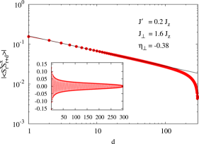
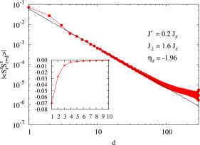
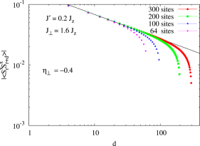
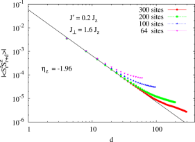
Figure 4: (Color online). $300$ site cluster, $J^{\prime}=0.2J_{z}$, $J_{\perp}=1.6J_{z}$. Example of static correlation functions for in-plane (left panel) and out-of-plane (right panel) channels plotted in logarithmic scale in the Spin-fluid-I (XXZ) phase. In the insets, the correlation functions are reported in linear scale.

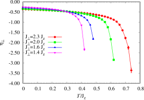
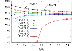
Figure 5: (Color online). Correlation functions in the Spin-Fluid-I phase at $J^{\prime}=0.2J_{z}$, $J_{\perp}=1.6J_{z}$ for different system sizes in the in-plane channel (left panel) and out-of-plane channel (right panel).

Figure 6: (Color online). $300$ site cluster. Spin-fluid-I phase: critical exponent of the in-plane correlations $\eta$ as a function of $J^{\prime}$ (left panel) and that of $J_{\perp}$ (right panel). The black curve labelled “exact” is the bosonization result from formula (4)

The above conditions give rise to the classical phase diagram depicted in Fig. 2 (left panel). In the absence of quantum correlations the system possesses a perfect long-range order, either commensurate or incommensurate, with periodicity vectors $q$ as shown in Fig. 2. There are three phases in the classical limit of the model (1) in the range $J^{\prime}>0$, $J_{\perp}>0$. The first one is the ferromagnetic phase (Ferro) with all spins fully polarized along the $z$-axis. The second phase is an in-plane Néel antiferromagnet, while the third one is the in-plane incommensurate spirally ordered phase with the periodicity vector $q=\arccos(J_{\perp}/4J^{\prime})$. The Ferro phase is separated from the Néel one by the line $J_{\perp}=J_{z}$, $J^{\prime}<J_{z}/4$, while the Néel phase is separated from the Spiral one by the line $J_{\perp}=4J^{\prime}$, $J_{\perp}>J_{z}$. Finally, the Spiral phase is separated from the Ferro one by the curve $J_{\perp}=\sqrt{8J^{\prime}(1-2J^{\prime})}$, $J_{z}/4<J^{\prime}<J_{z}/2$.

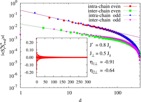
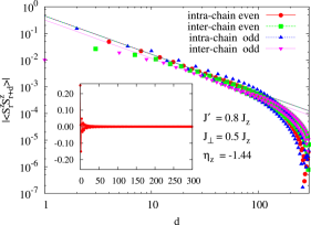
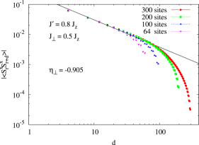
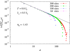
Figure 7: (Color online). $300$ site cluster, $J^{\prime}=0.8J_{z}$ $J_{\perp}=0.5J_{z}$. Example of static correlation functions for in-plane (left panel) and out-of-plane (right panel) channels plotted in logarithmic scale in the Spin-fluid-II phase. In the insets, the correlation functions are reported in linear scale.

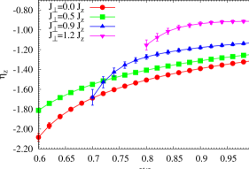
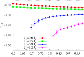
Figure 8: (Color online). Correlation lengths of the intra-chain even-distance correlation functions in Spin-Fluid-II phase at $J^{\prime}=0.5J_{z}$, $J_{\perp}=0.8J_{z}$ for different system sizes in the in-plane channel (left panel) and out-of-plane channel (right panel).

Figure 9: (Color online). $300$ site cluster. Spin-fluid-II phase: intra-chain critical exponent of the out-of-plane correlations $\eta_{z}$ (left panel) and that of the in-plane ones $\eta_{\perp}$ (right panel) as a function of $J^{\prime}$ for several lines with $J_{\perp}=$const.

4 Quantum phase diagram

Quantum fluctuations radically modify the classical picture. Long-range correlations with constant values of correlation functions, independent on distance, are substituted by either quasi-long-range ones with power-law behavior at large distances, or by short-range exponentially-decaying ones. For example, recently, it has been shown that quantum fluctuations appreciably reduce the ordering amplitude in the chiral phase of the model (1) supplied with the Dzyaloshinskii-Moriya interaction term furukawa_00 . In the quantum phase diagram of (1) we observe five phases as shown in the right panel of Fig.2.

In our previous studies Plekhanov_01 we have located the position of one of these phases (Ferro) within the range $0<J_{\perp}<J_{z}$ and $J^{\prime}\lesssim 0.31J_{z}$. Contrarily to the isotropic Heisenberg ferromagnet, where the ground state is $L+1$-times degenerate, in the anisotropic model (1) the ferromagnetic phase has only two degenerate ground states with all spins either “up” or “down”. Therefore, the Ferro phase is structurally identical to that of the classical phase diagram, the only difference being the shape of the phase boundary.

We now describe the remaining four phases of quantum phase diagram in Fig. 2, which we have found by use of the methods reported in Section 2.

4.1 Spin-fluid-I ($XXZ$-like) phase

Above the ferromagnetic phase ($J_{\perp}>J_{z}$) and for moderate values of $J^{\prime}$ (interpolating linearly the phase boundary between the Spin-Fluid-I and E-II phases in Fig. 2b, we can write for the boundary $J_{\perp}\sim 2.6J^{\prime}+0.35J_{z}$) we find a phase that we called Spin-fluid-I or $XXZ$-like because of its similarity to the ground state of AF $XXZ$ model. A typical behavior of the correlations in this phase is shown in Fig. 6. The relevant in-plane correlations are antiferromagnetic and power-law decaying, with periodicity vector $\pi$ and critical exponent $\eta_{\perp}$, which is a function of both $J_{\perp}$ and $J^{\prime}$:

$$\langle S^{x}_{r}S^{x}_{r+d}\rangle\sim(-1)^{d}d^{\eta_{\perp}}.$$

For what concerns the out-of-plane channel, the relevant correlations are always ferromagnetic:

$$\langle S^{z}_{r}S^{z}_{r+d}\rangle\sim-d^{\eta_{z}},$$

with the exponent close to $-2$. This fact confirms once again the analogy with $XXZ$ model.

Since DMRG deals with open boundary conditions (OBC), it is important to keep the boundary effects under control. With OBC, a two-site correlation function depends not only on the distance between the two sites, but also on the position of these sites. To minimize boundary effects, in the measurements of the two-site correlations, we choose these two sites as symmetric as possible with respect to the center of the cluster. In this way, the boundary effects, owing to the nonequivalence of the lattice points under OBC, can be overcome. We have studied the dependence of our results on the cluster size for a typical point in the Spin-fluid-I phase. As shown in Fig. 6, a progressive increase of $L$ increases the portion of points, lying on a straight line, common for all values of $L$ under investigation. The greater is the absolute value of $\eta_{\perp}$($\eta_{z}$), the smaller are the boundary effects, since for large a exponent the correlations decay fast enough on the scale of the cluster size $L$.

The dependence of $\eta_{\perp}$ on coupling constants along several lines with fixed values of $J_{\perp}$ and $J^{\prime}$ are shown in Fig. 6, left and right panels respectively. $\eta$ appears to be monotonically decreasing as a function of $J^{\prime}$. In the case when $J_{\perp}$ is constant, upon approaching the transition towards the E-II phase (see Fig. 2), $\eta_{\perp}$ shows a tendency to diverge to minus infinity. Peculiarly, all the curves cross at the same point around $J^{\prime}\approx 0.3J_{z}$, which means that at this point $\eta_{\perp}$ is independent of $J_{\perp}$.

In order to check the quality of our DMRG data, we compare our results for $\eta_{\perp}$ at the line $J^{\prime}=0$ with the known “exact” result of bosonization for the $XXZ$ model given by the formula (4). One can see from the right panel of Fig.6 that our points fall exactly on the bosonization line, meaning that our calculations (DMRG and the chosen cluster size) can access the bulk low-energy physics, described by the bosonization. Between $J^{\prime}=0.27J_{z}$ and $J^{\prime}=0.3J_{z}$ there is a change of convexity of $\eta_{\perp}(J_{\perp})$. At $J^{\prime}\approx 0.28J_{z}$, $\eta_{\perp}(J_{\perp})$ is approximately independent on $J_{\perp}$, especially for $J_{\perp}$ far from $1$, confirming the presence of a crossing point. The limiting value at $J_{\perp}\to\infty$ of the critical exponent for the in-plane correlations appears to be $-1/2$, as follows also from (4). This means that for $J_{\perp}$ large enough $J^{\prime}$ becomes always irrelevant.

4.2 Spin-fluid-II phase

We identify another spin-fluid phase in the range $J^{\prime}>0.43J_{z}$, $J_{\perp}<1.8J^{\prime}-0.2J_{z}$ i.e. when $J^{\prime}$ becomes dominant, while the NN interactions (parameterized by $J_{\perp}$ and $J_{z}$) become marginal. In Fig. 9 we report a typical correlation picture in the Spin-fluid-II phase, while the raw data for both in-plane and out-of-plane correlation functions are shown in the respective insets. It is more convenient to plot the correlation functions separating the inter- and intra-chain parts. Both in- and out-of-plane correlation functions have antiferromagnetic character in the intra- and inter-chain channels with periodicity vector $q\sim\pi/2$. The power-law decay of the correlations becomes clear after applying the logarithmic scale on both axes. Although the dominant NNN interaction ($J^{\prime}$) is isotropic, the corrections coming from the anisotropic NN ones ($J_{z}$, and $J_{\perp}$) induce anisotropy in the correlations.

The out-of-plane correlations appear to have the same exponent $\eta_{z}$ for both intra- and inter-chain correlations. Moreover, for the intra-chain correlations, there is an additional modulation by a harmonic term $\sim(1+\alpha\sin(2\pi x/4))$, where $x$ is the distance along a leg of the ladder and $\alpha\ll 1$. Such modulation, might be a trace of a less-relevant correlations (i.e. of a correlation with smaller exponent) which we are not able to measure directly. Contrarily to the out-of-plane channel, in the in-plane one the exponents of intra- ($\eta_{\perp 1}$) and inter-chain ($\eta_{\perp 2}$) correlations appear to be slightly different, as shown in Fig. 9. The cluster-size dependence of the intra-chain correlations is shown in Fig. 9. Once again, by increasing the system size $L$, the power-law character of the correlations becomes more and more evident. The convergence to the thermodynamic limit, however, is somewhat slower in comparison with the Spin-Fluid-I phase (see Fig.9), since now we are measuring the correlations along a leg of the ladder and the maximum distance along a leg is only half of the system size.

The critical exponents for the intra- and inter-chain correlations are not universal and depend on the particular values of $J^{\prime}$ and $J_{\perp}$. $J^{\prime}$ dependence of the intra-chain correlation exponents for in-plane $\eta_{\perp}$ and out-of-plane $\eta_{z}$ is shown in Fig. 9. For $J_{\perp}<0.9,J_{z}$ $\eta_{z}<-1$ and $\eta_{\perp}>-1$, while for $J_{\perp}>0.9J_{z}$ $\eta_{z}>-1$ and $\eta_{\perp}<-1$. When $J^{\prime}$ increases, both exponents tend to $-1$ as in this case the system resembles more and more the $XXZ$ model on two noninteracting legs.

4.3 E-I and E-II phases

The two phases E-I and E-II are characterized by the presence of at least one exponentially-decaying correlation function. Actually, the issue whether a gap is present in the system’s spectrum is subtle and would require a comprehensive study of all possible excitations.

The two phases (E-I, E-II) exhibit qualitatively different correlations and the transition line between them goes from the point ($J^{\prime}=J_{z}/4$, $J_{\perp}=J_{z}$) to the point ($J^{\prime}=0.41J_{z}$, $J_{\perp}=0.5J_{z}$), as shown in Fig. 2. The transition lines are determined by the behavior of the correlation functions. In a massless mode, the correlation functions are linear in the $\log$-$\log$ scale (power-law decay), while for a massive mode they are linear in the semi-$\log$ scale (exponential decay).

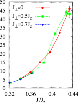
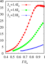
Figure 10: (Color online). $300$ site cluster. $J^{\prime}$ dependence of the correlation lengths for the in-plane correlations in the E-I phase (left panel) and for the out-of-plane ones in the E-II phase (right panel) for several values of $J_{\perp}$. Shown in this panel are the correlations along the legs ($d_{0}$ and $d_{2}$ sequences as explained in the text). Lines are guides to the eye.

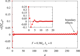
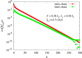
Figure 11: (Color online). $300$ site cluster. A sample of the correlations behavior in the E-I phase. Left panel: distance dependence of the out-of-plane static spin form factor. Short-range part of the correlations is shown in the inset. The shift due to finite magnetization $m=0.06$ is equal to $m^{2}=0.0036$ for the given values of $J^{\prime}$ and $J_{\perp}$. Right panel: semi-log plot of the in-plane spin form-factor. Intra- and inter-chain correlations have slightly different correlation lengths. Boundary effects manifest starting from approx. $d\gtrsim 250$. Lines are guides to the eye.

The first phase (E-I) is located in the region $0.31J_{z}<J^{\prime}<0.43J_{z}$, $0<J_{\perp}<J_{z}$. E-I is adjacent to the ferromagnetic phase and shows finite magnetization in the vicinity of the transition line, which gradually goes to zero for $J^{\prime}\gtrsim 0.35J_{z}$. In the E-I phase, residual ferromagnetic correlations induce a very complex structure of the static spin form factor in the $z$-direction. In addition to the residual finite magnetization, which shifts up the whole plot of $\langle S^{z}_{r}S^{z}_{r+d}\rangle$, the boundary effects are enhanced with respect to what we find in the other phases and in the in-plane channel. That is why we explore this phase on clusters of the maximal reachable size on our machines: $300$ sites. At short distances ($d<20$), in the out-of-plane channel the correlations are dominated by an exponential incommensurate contribution, as shown in the left panel of Fig. 11. Qualitatively different behavior appears for $d>20$. At medium distances ($20<d<250$) we observe incommensurate long-range correlations with apparently no decay. Finally, when the spins are situated at the opposite sides of the cluster, the correlations between them grow as the spins approach the borders of the cluster, being this behavior a clear evidence of a boundary effect.

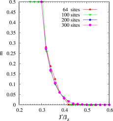
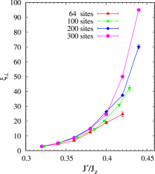
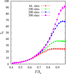
Figure 12: (Color online). $m$ - magnetization per site (left panel) and $\xi_{\perp}$ - correlation length of the in-plane correlations (middle panel) as a function of $J^{\prime}$ at $J_{\perp}=0.5J_{z}$ in the E-I phase for different system sizes. Right panel: $\xi_{z}$ - correlation length of the out-of-plane correlations in the E-II phase as a function of $J^{\prime}$ for different system sizes.

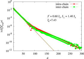
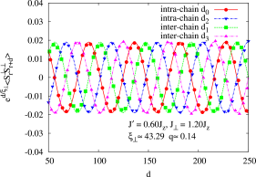
Figure 13: (Color online). $300$ site cluster. A sample of the correlations behavior in the E-II phase. Left panel: semi-log plot of the out-of-plane spin form-factor. Both intra- and inter-chain correlations fit the same line. For $d\gtrsim 100$, $|\langle S^{z}_{r}S^{z}_{r+d}\rangle|\lesssim 10^{-7}$, which is less than the accuracy of our DMRG method and such data are reported solely for the sake of completeness and reproducibility. Right panel: in-plane spin form-factor multiplied by the exponential pre-factor $e^{d/\xi}$. The points sequences fit quite well on the cosine functions with different phase shifts and with the incommensurate periodicity vector $q=0.14$. Only distances where the exponential-decaying behavior is established are shown. Lines are guides to the eye.

As it can be seen from the right panel of Fig. 11, the in-plane correlations exhibit exponential decay. As we have already mentioned, the model (1) can be also considered as a zig-zag ladder. Hence, there could be an a priori distinction between intra- and inter-chain correlations. The correlations we measured distinguish whether the two sites stay on the same leg or not. The inter-chain in-plane correlations have smaller correlation length with respect to the intra-chain ones, and go gradually to zero as $J_{\perp}\to 0$, since in that case the two legs of the ladder remain coupled only in the $z$-channel. In the left panel of Fig. 10, we plot the $J^{\prime}$ dependence of the in-plane intra-chain correlation length $\xi_{\perp}$ for several values of $J_{\perp}$. $\xi_{\perp}(J^{\prime})$ appears to be independent of $J_{\perp}$ at least close to the transition line Ferro$\to$E-I. The maximal value reached by $\xi_{\perp}$ ($50$ lattice constants) on approaching the transition E-I$\to$Spin-fluid-II (along $J_{\perp}=0.0$ and $0.5J_{z}$ lines) is much greater than that ($10$ lattice constants) reached at the transition E-I$\to$E-II (along $J_{\perp}=0.7J_{z}$ line).

The issue of finite magnetization in the E-I phase, rather unexpected, deserves a separate study through the finite-size scaling in order to conclude whether it might be a bulk feature.

In order to determine the residual magnetization, we have used the DMRG program with symmetry reduction of the Hilbert space into invariant subspaces with definite $S^{z}_{tot}$. In such a case, the residual magnetization at given values of $J_{\perp}$ and $J^{\prime}$ corresponds to the sector of $S^{z}_{tot}$ containing the global energy minimum. These results were subsequently verified by another DMRG program without symmetry reduction where at each point of the phase E-I the absolute value of the residual magnetization has been deduced from the sum of the $z-$component of spin-spin correlation functions on for all distances:

$$|m|=\frac{|\langle S^{z}_{tot}\rangle|}{L}=\frac{1}{L}\sqrt{\sum_{i,j}\langle S^{z}_{i}S^{z}_{j}\rangle}.$$ (9)

In (9) we have used the fact that in absence of the magnetic field and with rotational degeneracy broken $J_{\perp}\neq J_{z}$, the eigenstate with a $S^{z}_{tot}=\mathcal{M}$ is degenerate with respect to $S^{z}_{tot}=-\mathcal{M}$. Therefore, for the program without symmetry reduction a ground state with $S^{z}_{tot}=|\mathcal{M}|$ will be an arbitrary mixture of states with $S^{z}_{tot}=\mathcal{M}$ and $S^{z}_{tot}=-\mathcal{M}$, but $|S^{z}_{tot}|$ will have a definite value. In order to exclude that the residual magnetization in the E-I phase is a DMRG artifact caused by the difficulties to reach convergence in the proximity of a phase transition, we have performed a finite-size scaling analysis by means of Lanczos technique, free of DMRG truncation error, on clusters with up to 30 sites for both open and periodic boundary conditions. Lanczos data has confirmed DMRG ones: in the E-I phase, the finite magnetization has no tendency to disappear also in the thermodynamic limit.

In the E-I phase and for the values of $L$ accessible to us, we find a close relation between the finite residual magnetization and the correlation length $\xi_{\perp}$ in the in-plane channel, as shown in the left and middle panels of Fig. 12. Namely, the decrease of the magnetization per site is accompanied by the increase of $\xi_{\perp}$. The former appears to be almost size independent for $J^{\prime}<0.4J_{z}$. At $J^{\prime}>0.4J_{z}$, finite magnetization steps of height $1/L$ appear. This occurs because, for a finite cluster, the $z$-component of the total spin can only increment by one. The disappearance of magnetization is accompanied by the divergence of the correlation length $\xi_{\perp}$ in the in-plane channel (left and middle panels of Fig. 12). On increasing $J^{\prime}$, $\xi_{\perp}$ reaches a maximal value (of the order of $L/2$) at $J^{\prime}=0.42\div 0.44J_{z}$ and, for greater values of $J^{\prime}$, a power-law fit appears to be more appropriate.

Such behavior is surprisingly similar to what was found in the multi-magnon phase of the isotropic model (1) at $J^{\prime}>\frac{1}{4}J_{z}$ and in magnetic field drechsler_04 ; kecke_01 ; kecke_02 . Indeed, a state with $n$ magnons is characterized by a wave function with non-zero total magnetization equal to $\pm(L/2-n)$. It is worth noting that for $J^{\prime}>\frac{1}{4}J_{z}$ finite magnetization can exist in the isotropic model only in the presence of an external magnetic field, while in our case it can be induced by tuning the values of $J^{\prime}$ and $J_{\perp}$ for zero field. Increasing $J^{\prime}$ at fixed $J_{\perp}$ the total cluster magnetization decreases from $L/2$ to zero, implying that the total number of magnons increases from zero to $L$ (infinity in thermodynamic limit). In the case of the isotropic model in magnetic field, the low-lying excitations are generally formed of bound multi-magnon clouds and are gapless, while the in-plane correlation functions are expected to decay exponentially kecke_01 ; kecke_02 . If the multi-magnon scenario is realized also in our case is currently under investigation. As a matter of fact, the exponential decay of the in-plane correlations (see the left panel of Fig.11) is clearly in favor of this scenario.

In the E-II phase, when both $J^{\prime}$ and $J_{\perp}$ become large enough, the correlations change qualitatively. In this phase, the ratio $J_{\perp}/J^{\prime}$ is limited from below and above. The out-of-plane correlations exhibit an exponential decay as functions of the distance between any two sites, regardless whether they belong to the same or different legs (see left panel of Fig. 13). We have also investigated $J^{\prime}$ dependence of the out-of-plane intra-chain correlation length $\xi_{z}$ for several values of $J_{\perp}$ in the E-II phase, as reported in the right panel of Fig. 10. $\xi_{z}(J^{\prime})$ grows monotonically from the left border of the phase (transition Spin-fluid-I$\to$E-II) to the right one (transition E-II$\to$Spin-fluid-II). Such non-symmetric behavior implies radically different types of orders in the two massless phases.

The in-plane correlation function shows an exponential decay with a correlation length $\xi_{\perp}$ ($\xi_{\perp}=43.29$ for $J^{\prime}=0.6J_{z}$ and $J_{\perp}=1.2J_{z}$). Once multiplied by $e^{d/\xi_{\perp}}$, as shown in the right panel of Fig. 13, the correlation function presents incommensurate oscillations as a function of $d$ with periodicity vector $q$ ($q=0.14$ for $J^{\prime}=0.6J_{z}$ and $J_{\perp}=1.2J_{z}$) and a phase depending on ${\rm mod}(d,4)$ as follows. The whole set of distances $d\equiv|i-j|$ between any two sites $i$ and $j$ on a 1D cluster splits into four sequences:

$$d_{0}(l)=4l+0,\qquad 0,4,8,12,\dots$$

$$d_{1}(l)=4l+1,\qquad 1,5,9,13,\ldots$$

$$d_{2}(l)=4l+2,\qquad 2,6,10,14,\ldots$$

$$d_{3}(l)=4l+3,\qquad 3,7,11,15,\ldots$$

where $l=0,\ldots,24$ for a $300$ site cluster. One can easily verify by looking at Fig. 1 that the sequence $d_{0}(l)$ corresponds to the case when both $i$ and $j$ belong to the same leg and $i-j$ is even. Similarly, the sequence $d_{2}(l)$ comprises all the cases when both $i$ and $j$ belong to the same leg and $i-j$ is odd. The remaining two sequences $d_{1}(l)$ and $d_{3}(l)$ are realized when $i$ and $j$ belong to different legs. All four sequences appear to be modulated by the same harmonic term, but with different phases. Peculiarly, the phase shift between $d_{0}(l)$ and $d_{2}(l)$ equals to $\pi$ and the same does the phase shift between $d_{1}(l)$ and $d_{3}(l)$. Finally, the phases of $d_{0}(l)$ and $d_{1}(l)$ differ by $\pi/2$. Summarizing, we can conclude that the in-plane correlations of the E-II phase assume the following asymptotic form:

$$\langle S^{x}_{n}S^{x}_{n+d}\rangle\sim\exp(-d/\xi_{\perp})\cos(qd+\phi_{d}),$$ (10)

where $\phi_{d}=\frac{\pi}{2}{\rm mod}(d,4)$.

On a cluster of $100$ sites, the out-of-plane correlation length $\xi_{z}$ approaches its saturation value of about $\xi^{c}_{z}\sim 35a$, while the system undergoes the phase transition towards the Spin-Fluid-II phase, and hence $\xi^{c}_{z}/L\sim 0.35$ for $L=100$. This value should be compared to $L/2=50$ since we are speaking about the intra-chain correlations. In the right panel of Fig.12 we report the $J^{\prime}$-dependence of $\xi_{z}$ for different system sizes. The ratio $\xi^{c}_{z}/L$ ranges from $0.3$ for $L=300$ to $0.375$ for $L=64$ while the “uncertainty” range, i.e. the width of the transition on a finite system, decreases as expected.

The phase E-II comprises the isotropic line for the values $J^{\prime}\in[0.25J_{z},0.7J_{z}]$. In this region, an ”astronomically small” gap itoi has been predicted by means of bosonization. The vanishing value of the predicted gap precludes any possibility of its numerical observation. Indeed, in the E-II phase, finite-size scaling shows that the excitation gaps, both in singlet sector (containing the ground state) and between triplet and singlet sectors converge to zero in our DMRG calculations (not shown).

Currently, by using the numerical tools to our disposition, we can not discriminate between the two hypotheses: i) that there indeed exists a tiny gap in the spectrum, which can not be directly observed numerically, and ii) that the system is gapless, but the excitations associated with the correlation functions studied have a gap.

5 conclusions

We have performed an extensive numerical study of the model (1) within the following range of the Hamiltonian parameters: $J_{z}=1$, $0<J_{\perp}<2.5$, $0<J^{\prime}<1.0$. We have constructed a zero-temperature phase diagram based on the DMRG calculations for $64,100,200,300$ site system with open boundary conditions.

We have identified several phases within this phase diagram, based on the behavior at large distances of the correlation functions. We have found two phases with quasi-long-range behavior, among which one appears to be a generalization of the ground state of $XXZ$ model, and another possesses rather complex correlation picture, which distinguishes between intra- and inter-chain distances. We have discovered two phases with exponentially-decaying correlation functions. One of them (E-II) separates the two massless phases, while the other (E-I) divides a massless phase from the ferromagnetic one. Although these two phases present qualitatively different correlations, they share a common feature. Both of them develop when one of the NN couplings is less efficient respect to the other and to $J^{\prime}$. Indeed, in the phase E-I, $J_{\perp}$ is limited respect to the other couplings, while in E-II the relative weight of $J_{z}$ goes to zero with respect to $J_{\perp}$ and $J^{\prime}$. A further insight into the nature of the phases found in this manuscript can be obtained by studying more specific properties of their ground states, like entanglement, or by measuring various more sophisticated correlation functions e.g. spiral or dimer ones kaburagi_00 ; kaburagi_01 ; kaburagi_02 . Such work is currently in progress.

For what concerns real materials, for ${\rm Rb_{2}Cu_{2}Mo_{3}O_{12}}$ we have hase $J^{\prime}\approx 0.37J_{z}$ and from Fig. 2 we can conclude that its ground state should be either in E-I or E-II phase depending on the anisotropy. The same conclusion holds also for ${\rm Li_{2}ZrCuO_{4}}$ ($J^{\prime}\approx 0.26J_{z}$), ${\rm Pb_{2}[CuSO_{4}(OH)_{2}]}$ ($J^{\prime}\approx 0.43J_{z}$) and ${\rm Cs_{2}Cu_{2}Mo_{3}O_{12}}$ ($J^{\prime}\approx 0.38J_{z}$) as estimated in the Ref. drechsler_02 . ${\rm NaCu_{2}O_{2}}$ was found drechsler_01 to have $J^{\prime}\approx 2J_{z}$ and assuming that the anisotropy is not too strong we conclude that its ground state is in the Spin-Fluid-II phase. Finally, for ${\rm LiCuVO_{4}}$ the estimates for $J^{\prime}$ range from $2.4J_{z}$ to $3.5J_{z}$. These values, under the assumption of weak anisotropy, bring us again to the Spin-fluid-II phase. Recently, a new value of $J^{\prime}\sim 0.3J_{z}$ for Li₂CuO₂ has been deduced by means of various methods drechsler_05 ; drechsler_06 , in contrast to the value $J^{\prime}=0.62J_{z}$ previously known mizuno_00 . If one approximates Li₂CuO₂ by non-interacting chains each described by Hamiltonian (1), then this material should belong either to E-I or E-II phase depending on the actual anisotropy (still under debate).

- (1) M. Hase, H. Kuroe, K. Ozawa, O. Suzuki, H. Kitazawa, G. Kido, T. Sekine, Phys. Rev. B 70, 104426 (2004)
- (2) S.L. Drechsler, J. Richter, A.A. Gippius, A. Vasiliev, A.A. Bush, A.S. Moskvin, J. Malek, Y. Prots, W. Schnelle, H. Rosner, Europhys. Lett. 73, 83 (2006)
- (3) M. Enderle, C. Mukherjee, B. Fak, R.K. Kremer, J.M. Broto, H. Rosner, S.L. Drechsler, J. Richter, J. Malek, A. Prokofiev et al., Europhys. Lett. 70, 237 (2005)
- (4) H.A. Krug von Nidda, L.E. Svistov, M.V. Eremin, R.M. Eremina, A. Loidl, V. Kataev, A. Validov, A. Prokofiev, W. Aßmus, Phys. Rev. B 65, 13445 (2002)
- (5) A.N. Vasil’ev, L.A. Ponomarenko, H. Manaka, I. Yamada, M. Isobe, Y. Ueda, Phys. Rev. B 64, 024419 (2001)
- (6) T. Tonegawa, I. Harada, J. Phys. Soc. Jpn. 56, 2153 (1987)
- (7) S. Hirata, K. Nomura, Phys. Rev. B 61, 9453 (2000)
- (8) F.D.M. Haldane, Phys. Rev. B 25, 4925 (1982)
- (9) E. Plekhanov, A. Avella, F. Mancini, Phys. Rev. B 74, 115120 (2006)
- (10) S.R. White, I. Affleck, Phys. Rev. B 54, 9862 (1996)
- (11) C.K. Majumdar, J. Phys. C 3, 911 (1970)
- (12) T. Hamada, J.K.S. Nakagawa, Y. Natsume, J. Phys. Soc. Jpn. 57, 1891 (1988)
- (13) F.D.M. Haldane, Phys. Lett. A 93, 464 (1983)
- (14) F.D.M. Haldane, Phys. Rev. Lett. 50, 1153 (1983)
- (15) E. Dagotto, Rev. Mod. Phys. 66, 763 (1994)
- (16) H.H. Hung, C.D. Gong, Phys. Rev. B 71, 054413 (2005)
- (17) I. Affleck, in Fields, Strings and Critical Phenomena, edited by E. Brezin, J. Zinn-Justin (North-Holland, Amsterdam, 1990)
- (18) H.J. Schultz, in Proceedings of the Les Houches Sunner School LXI: Mesoscopic Quantum Physics, edited by E. Ackermans, G. Montambaux, J.L. Pichard, J. Zinn-Justin (Elsevier, Amsterdam, 1995), p. 533
- (19) M. Azuma, Z. Hiroi, M. Takano, K. Ishida, Y. Kitaoka, Phys. Rev. Lett. 73, 3463 (1994)
- (20) K. Kojima, A. Keren, G.M. Luke, B. Nachumi, W.D. Wu, Y.J. Uemura, M. Azuma, M. Takano, Phys. Rev. Lett. 74, 2812 (1995)
- (21) C. Itoi, S. Qin, Phys. Rev. B 63, 224423 (2001)
- (22) K. Nomura, K. Okamoto, J. Phys. A 27, 5773 (1994)
- (23) R.D. Somma, A.A. Aligia, Phys. Rev. B 64, 024410 (2001)
- (24) R. Jafari, A. Langari, Phys. Rev. B 76, 014412 (2007)
- (25) R. Bursill, G.A. Gehring, D.J.J. Farrnell, J.B. Parkinson, T. Xiang, C. Zeng, J. Phys.: Condens. Matter 7, 8605 (1995)
- (26) A.A. Nersesyan, A.O. Gogolin, F.H.L. Essler, Phys. Rev. Lett. 81, 910 (1998)
- (27) M. Kaburagi, H. Kawamura, T. Hikihara, J. Phys. Soc. Jpn. 68, 3185 (1999)
- (28) T. Hikihara, M. Kaburagi, H. Kawamura, Phys. Rev. B 63, 174430 (2001)
- (29) T. Hikihara, M. Kaburagi, H. Kawamura, Can. J. Phys. 79, 1581 (2001)
- (30) D.V. Dmitriev, V.Y. Krivnov, Phys. Rev. B 77, 024401 (2008)
- (31) T. Vekua, A. Honecker, H.J. Mikeska, F. Heidrich-Meisner, Phys. Rev. B 76, 174420 (2007)
- (32) F. Heidrich-Meisner, A. Honecker, T. Vekua, Phys. Rev. B 74, 020403 (2006)
- (33) F. Heidrich-Meisner, I.P. McCulloch, A.K. Kolezhuk, Phys. Rev. B 80, 144417 (2009)
- (34) J. Sudan, A. Lüscher, A.M. Läuchli, Phys. Rev. B 80, 140402 (2009)
- (35) N. Kitanine, J.M. Maillet, V. Terras, Nucl. Phys. B 554, 647 (1999)
- (36) N. Kitanine, J.M. Maillet, V. Terras, Nucl. Phys. B 567, 554 (2000)
- (37) I. Affleck, J. Phys. A 31, 4573 (1998)
- (38) S. Lukyanov, A. Zamolodchikov, Nucl. Phys. B 493, 571 (1997)
- (39) A. Avella, F. Mancini, E. Plekhanov, Conden. Matt. Phys. 9, 485 (2006)
- (40) E. Plekhanov, A. Avella, F. Mancini, Physica B 403, 1282 (2008)
- (41) S.R. White, Phys. Rev. Lett. 69, 2863 (1992)
- (42) S.R. White, Phys. Rev. B 48, 10345 (1993)
- (43) S. Furukawa, M. Sato, Y. Saiga1, S. Onoda, J. Phys. Soc. Jpn. 77, 123712 (2008)
- (44) R.O. Kuzian, S.L. Drechsler, Phys. Rev. B 75, 024401 (2007)
- (45) T. Hikihara, L. Kecke, T. Momoi, A. Furusaki, Phys. Rev. B 78, 144404 (2008)
- (46) L. Kecke, T. Momoi, A. Furusaki, Phys. Rev. B 76, 060407 (2007)
- (47) S.L. Drechsler, J. Richter, R. Kuzian, J. Malek, N. Tristan, B. Buchner, A. Moskvin, A. Gippius, A. Vasiliev, O. Volkova et al., J. Mag. Mag. 316, 306 (2007)
- (48) S.L. Drechsler, J. Malek, S. Nishimoto, U. Nitzsche, R. Kuzian, H. Eschrig, H. Rosner, Journal of Physics: Conference Series 145, 012060 (2009)
- (49) W.E.A. Lorenz, R.O. Kuzian, S.L. Drechsler, W.D. Stein, N. Wizent, G. Behr, J. Malek, U. Nitzsche, H. Rosner, A. Hiess et al., Europhys. Lett. 88, 37002 (2009)
- (50) Y. Mizuno, T. Tohyama, S. Maekawa, T. Osafune, N. Motoyama, H. Eisaki, S. Uchida, Phys. Rev. B 57, 5326 (1998)