Three-Dimensional Relativistic MHD Simulations of the Kelvin-Helmholtz Instability: Magnetic Field Amplification by a Turbulent Dynamo

Abstract

Magnetic field strengths inferred for relativistic outflows including gamma-ray bursts (GRB) and active galactic nuclei (AGN) are larger than naively expected by orders of magnitude. We present three-dimensional relativistic magnetohydrodynamics (MHD) simulations demonstrating amplification and saturation of magnetic field by a macroscopic turbulent dynamo triggered by the Kelvin-Helmholtz shear instability. We find rapid growth of electromagnetic energy due to the stretching and folding of field lines in the turbulent velocity field resulting from non-linear development of the instability. Using conditions relevant for GRB internal shocks and late phases of GRB afterglow, we obtain amplification of the electromagnetic energy fraction to $\epsilon_{B}\sim 5\times 10^{-3}$. This value decays slowly after the shear is dissipated and appears to be largely independent of the initial field strength. The conditions required for operation of the dynamo are the presence of velocity shear and some seed magnetization both of which are expected to be commonplace. We also find that the turbulent kinetic energy spectrum for the case studied obeys Kolmogorov’s $5/3$ law and that the electromagnetic energy spectrum is essentially flat with the bulk of the electromagnetic energy at small scales.

1. Introduction

Strong magnetic fields are required in GRB and AGN outflows to enable sufficient production of non-thermal radiation. Synchrotron models for GRB afterglow emission require magnetic field strengths many orders of magnitude larger than expected in smoothly shock compressed circum-burst medium. For the prompt GRB emission, magnetic field may be advected from the central engine to the emission region, but the degree of advected magnetization is uncertain and may be small. The source of sufficiently strong magnetic field responsible for non-thermal GRB emission has thus remained a mystery, and a similar situation exists for AGN. Possible mechanisms capable of generating magnetic fields in relativistic collisionless shocks are plasma instabilities, such as the Weibel two-stream instability (Gruzinov & Waxman, 1999; Medvedev & Loeb, 1999). Recent plasma simulations using the particle-in-cell (PIC) method (Buneman, 1993) have demonstrated magnetic field generation in relativistic collisionless shocks (Nishikawa et al., 2003; Spitkovsky, 2008). However, the size of the simulation boxes is orders of magnitude smaller than the GRB and AGN emitting regions. It remains unclear whether fields generated on scales of tens of plasma skin depths, as in the current PIC simulations, will persist at sufficient strength, or at all, on radiation emission scales. In addition, the recent plasma simulations (Spitkovsky, 2008) are two-dimensional hence missing intrinsically three-dimensional effects which may be necessary for dynamo operation (Gruzinov, 2008). Thus it is far from clear that magnetized regions with size scales and magnitudes inferred for AGN and GRBs can be generated by plasma instabilities alone.

Another possibility is that weak magnetic field is greatly amplified by a magnetohydrodynamic (MHD) turbulent dynamo (Kazantsev, 1968; Kulsrud & Anderson, 1992; Boldyrev & Cattaneo, 2004; Gruzinov, 2008). In our scenario the turbulence is driven by non-linear development of the Kelvin-Helmholtz instability present due to velocity shear. Shear is naturally expected in realistic explosive outflows due to intermittency and inhomogeneity in the outflow itself and in the surrounding medium. Collisions in GRB internal shocks, for example, likely occur between blobs of differing size and shape resulting in oblique shocks and vorticity generation in the post-shock flow (Goodman & MacFadyen, 2008). In jets, shear is intrinsic between a fast jet core and the surrounding “cocoon” which is often turbulent due to Kelvin-Helmholtz instability. Shocks launched into a clumpy medium, as expected, for example, in the regions surrounding massive stars, will lead to significant vorticity generation and velocity shear during clump shocking (Goodman & MacFadyen, 2008) or from ion streaming (Couch, Milosavljević & Nakar, 2008). In these cases the Kelvin-Helmholtz instability is likely to generate turbulence from the shear flow. These flows are highly ionized and as such are expected to contain some magnetic field however weak.

In this letter, we present high-resolution, three-dimensional numerical simulations of relativistic MHD demonstrating amplification of weak magnetic fields by Kelvin-Helmholtz instability induced turbulence. This process is demonstrated to be viable as the origin of strong magnetic fields present behind relativistic collisionless shocks of astrophysical jets in AGN and GRBs. Our simulations also allow us to study the basic properties of turbulence in the largely unexplored relativistic MHD case. In § 2 we describe the initial setup of our simulations. In § 3 we present the simulation results. We further discuss the results in § 4.

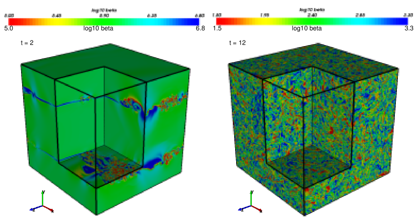
Figure 1.— Plasma $\beta$, the ratio of gas pressure to the magnetic pressure, for Model A-1024. Results at $t=2$ and $t=12$ are shown in the left and right panel, respectively. $1024^{3}$ numerical cells are used in this calculation for which the numerical box size and light crossing time is $1$. At $t=0$, the speed of the gas is set to $\mathrm{v}_{x}=0.5$ in the top and bottom quarters of the box and $\mathrm{v}_{x}=-0.5$ in the middle half of the box, with small perturbations added. Initially, the box is filled with a weak magnetic field, which corresponds to $\beta=2\times 10^{6}$. By $t=2$, vortices due to the Kelvin-Helmholtz instability are clearly visible. The instability grows and the magnetic field is amplified by stretching and folding of field lines. By $t=12$, the gas has become fully turbulent due to the instability and the plasma beta is highly variable with values as low as $\sim 10$ in some regions.

2. MHD Equations and Initial Setup

The system of special relativistic MHD (SRMHD) is governed by the equations of mass conservation, energy-momentum conservation and magnetic induction, respectively given by

$$\nabla_{\nu}\rho u^{\nu}=0,$$ (1)

$$\nabla_{\nu}T^{\mu\nu}=0,$$ (2)

$$\frac{\partial}{\partial{t}}\vec{B}=\vec{\nabla}\times(\vec{v}\times\vec{B}).$$ (3)

Here $\rho$ is the mass density in the local rest frame, $u^{\nu}$ is the four-velocity, $T^{\mu\nu}$ is the energy-momentum tensor, $\vec{B}$ is the magnetic field three-vector in the lab frame, and $\vec{v}$ is the three-velocity. The energy-momentum tensor, which includes both the fluid and electromagnetic parts is given by,

$$T^{\mu\nu}=\rho hu^{\mu}u^{\nu}+Pg^{\mu\nu}+(u^{\mu}u^{\nu}+\frac{1}{2}g^{\mu\nu})b^{2}-b^{\mu}b^{\nu},$$ (4)

where $P$ is the pressure, $g^{\mu\nu}$ is the metric, $b^{\mu}$ is the four-vector of the magnetic field measured in the local rest frame, and $h\equiv 1+e+P/\rho$ is the specific enthalpy here $e$ is the specific internal energy. Units in which the speed of light is set to $c=1$ are used, and the magnetic field is redefined to absorb a factor of $1/\sqrt{4\pi}$. The system is closed by an equation of state. Furthermore, there is the solenoidal constraint $\vec{\nabla}\cdot\vec{B}=0$.

A mildly relativistic and weakly magnetized shear flow with zero net momentum was set up as the initial condition. A three-dimensional grid $(x,y,z)$ in Cartesian coordinates was used with periodic boundary conditions applied in all directions. The dimensionless size of the box was $1$ in each direction and the center of the box was at $(0,0,0)$. Initially the numerical box was filled with relativistically hot gas of constant pressure of $P_{0}=1$ and constant density of $\rho_{0}=1$. The equation of state was assumed to be an ideal gas with gamma-law, $P=(\gamma-1)\rho e$, with a constant adiabatic index $\gamma=4/3$. A shearing flow initial condition was imposed with the velocity in the top quarter ($y>0.25$) and bottom quarter ($y<-0.25$) of the box in the positive $x$-direction at a speed of $v_{x}=0.5$ and in the negative $x$-direction at a speed of $v_{x}=-0.5$ in the middle half ($-0.25<y<0.25$) of the box. This corresponds to a shear flow with relative Lorentz factor of $2.29$. The system had an initially weak magnetic field of $B_{x}=10^{-3}$ and $10^{-2}$ for Models A and E, respectively. Small velocity perturbations were added of the form,

$$v_{i1}=a_{p}\cos{(\mathbf{k}\cdot\mathbf{r}+\phi_{i})},$$ (5)

where $i$ denotes $x$-, $y$- and $z$-direction, $\mathbf{r}$ is the position and $\phi_{i}$ is a random number in the range of $[0,2\pi)$. The amplitude of the perturbation is set to $a_{p}=0.01$. The wave vector $\mathbf{k}$ is given by $\mathbf{k}=2\pi(\cos{\theta_{p}}\mathbf{e}_{x}+\sin{\theta_{p}}\mathbf{e}_{y})$, here $\theta_{p}$ is set to $0.05$. The initial perturbation is roughly a single mode. The relativistic sound speed in the initial models is $c_{s}=0.516$ and the flow speed is $0.5$ (with perturbations of $\leq 0.01$). Thus the initial shear flow is transonic. Also the initial conditions of the shear flow correspond to $\beta=1.2\times 10^{6}$ and $1.2\times 10^{4}$ for Models A and E, respectively. Here the plasma beta is $\beta=P/P_{m}$, where $P$ is gas pressure and $P_{m}$ is magnetic pressure. In the absence of magnetic field, Kelvin-Helmholtz instability develops no matter how small or large the velocity shear is, whereas strong magnetic field can suppress the instability. This is true in 3D even for supersonic flow speeds because there are always directions along which the shear flow component is subsonic (Landau & Lifshitz, 1959). Because the initial field in our models is small and dynamically unimportant, Kelvin-Helmholtz instability develops in our 3D simulations.

3. Results

The SRMHD simulations in this letter were performed with the general relativistic MHD code Nvwa (Zhang & Wang in prep). The three-dimensional numerical simulations were run with various resolutions: $512^{3}$, $768^{3}$ and $1024^{3}$ numerical cells. We use A-n and E-n to denote Models A and E, respectively, where n stands for the number of numerical cells in each dimension. For example, Model A-1024 stands for Model A with a resolution of $1024^{3}$ numerical cells.

3.1. Amplification of Magnetic Fields

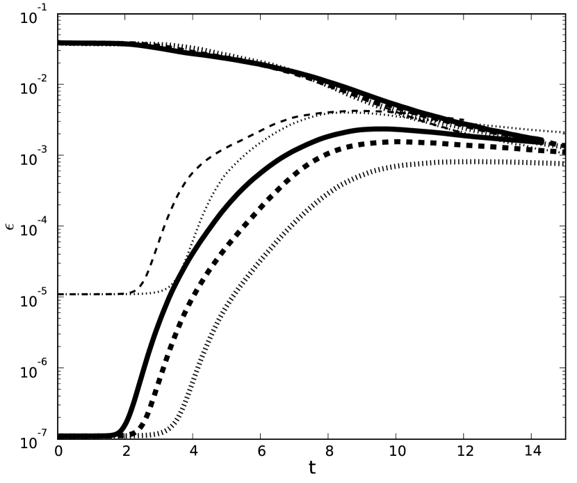
Figure 2.— Ratio of electromagnetic and kinetic energy to total energy as a function of time for Models A and E. The lines for kinetic energy start at $\epsilon\sim 4\times 10^{-2}$ at $t=0$ for all models, whereas the lines for electromagnetic energy start at $\epsilon\sim 10^{-7}$ and $10^{-5}$ for Models A and E respectively. Different lines are for different resolutions: $1024^{3}$ cells (solid line), $768^{3}$ cells (dashed lines), and $512^{3}$ cells (dotted lines). Models A and E are shown in thick and thin lines, respectively. The ratio of electromagnetic energy to total energy ($\epsilon_{B}$) grows due to growth of the Kelvin-Helmholtz instability and ensuing turbulence. The electromagnetic energy saturates at $t\sim 9$ depending upon the model and resolution. The kinetic energy decays over time, and it becomes comparable to electromagnetic energy at $t\sim 14$ for Model A-1024.

In all models the initial discontinuity in velocity triggered Kelvin-Helmholtz instability. Two snapshots of Model A-1024 are shown in Fig. 1. Kelvin-Helmholtz vortices start to appear on the plane of the velocity discontinuity after $\sim 2$ light crossing times of the numerical box due to the roll-up of the shear flow. The magnetic field at the shear layer is being folded and twisted by the vortical fluid motion. The strength of the magnetic field starts to increase rapidly, growing exponentially as shown in Fig. 2. As the instability evolves, more and more gas is turned into a state of turbulence. At about $t\sim 7$, the whole box has become fully turbulent, and the electromagnetic energy starts to saturate. The turbulence eventually decays because there is no bulk shear flow left to further drive the turbulence. Fig. 2 shows the evolution of the ratio of the electromagnetic energy to total energy for Models A and E at various levels of resolution, here the total energy does not include rest mass energy. Also shown in Fig. 2 is the ratio of the kinetic energy to total energy. Note that the kinetic energy decays faster than the electromagnetic energy. For Model A-1024, the electromagnetic energy becomes comparable to kinetic energy at $t\sim 14$.

The spatial structure of plasma beta for Model A-1024 is shown in Fig 1 at two times. The structure is clumpy and filamentary as expected for magnetic fields amplified by a turbulent dynamo. At the stage of full turbulence, the average ratio of the electromagnetic energy to total energy is $\epsilon_{B}\sim 2\times 10^{-3}$ for Model A-1024, whereas maximum values of $\epsilon_{B,\mathrm{max}}\sim 0.2$ exist throughout the box. Thus magnetic field is very strong in local patches of the turbulence. These strongly magnetized clumps are preferably elongated along the magnetic field direction due to the intrinsic anisotropy of MHD turbulence (Goldreich & Sridhar, 1995). It should be noted that there is no overall magnetic flux except for a very low magnetic flux in $x$-direction present in the initial conditions. The strength of the magnetic field is a result of folding and twisting of existing field lines by turbulent motions. This process increases magnetic energy density without increasing total magnetic flux.

To study the effects of numerical resolution and initial magnetic field strength on the level of magnetization that can be reached, we have run a series of calculations, Models A-768, A-512, E-768 and E-512 for comparison (Fig. 2). As expected, the onset of the instability is delayed and the saturated level of magnetization is lower for lower resolution runs due to their higher numerical diffusivity. The maximal overall ratio of the electromagnetic energy to total energy reaches $8.2\times 10^{-4}$, $1.6\times 10^{-3}$ and $2.4\times 10^{-3}$ for Models A-512, A-768 and A-1024, respectively. For Model E, which started with higher initial magnetic field, the final magnetization is higher than that of Model A as we also expected because less stretching and folding is required for reaching the same magnetic field strength. The maximal overall ratio of the electromagnetic energy to total energy reaches $4.1\times 10^{-3}$ and $4.5\times 10^{-3}$ for Models E-512 and E-768, respectively. But it should be noted that the two orders of magnitude difference in the initial fields causes only a factor of $<3$ in the final ratio of the electromagnetic energy to total energy. These results suggest that the “true” answer is $\epsilon_{B}\sim 5\times 10^{-3}$ for the chosen conditions.

3.2. MHD Turbulence

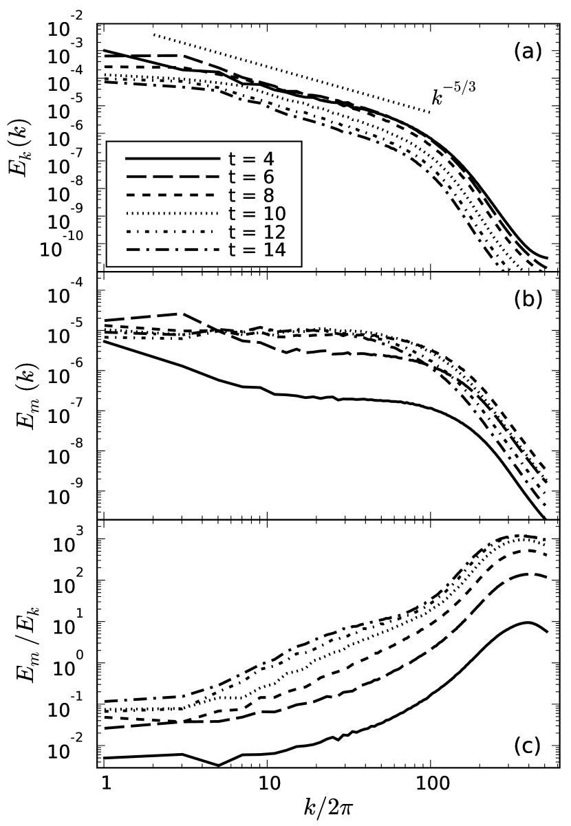
Figure 3.— Spherically-integrated spectrum of (a) kinetic energy (top) and (b) electromagnetic energy (middle), and (c) ratio of electromagnetic spectrum to kinetic energy spectrum (bottom) for Model A-1024. Different lines are for different times: $t=4$ (solid lines), $t=6$ (long dashed lines), $t=8$ (short dashed lines), $t=10$ (dotted lines), $t=12$ (short dash-dotted lines), and $t=14$ (long dash-dotted lines). Also shown in (a) is a line representing the power law $E(k)\sim k^{-5/3}$ for comparison.

We now analyze the properties of decaying mildly relativistic adiabatic MHD turbulence using the data of Model A-1024. The initial flow is mildly relativistic and transonic with shear velocity of $0.5$ corresponding to a Lorentz factor of $\Gamma_{0}=1.15$. During the evolution, the velocities of plasma elements decrease due to dissipation into heat and the work done to stretch and fold magnetic field lines. The typical velocities in Model A-1024 at $t=4$, $8$, $14$, are about $0.4$, $0.3$ and $0.1$, with a standard deviation of $0.1$, $0.1$ and $0.05$ respectively. Hence, the MHD turbulence in our simulations is mostly subsonic except for at the very beginning.

We define the kinetic energy spectrum $E_{k}(k)$ as

$$\int{E_{k}(k)dk}=\langle\rho\Gamma(\Gamma-1)\rangle,$$ (6)

where $\Gamma$ is the Lorentz factor, and the electromagnetic energy spectrum $E_{m}(k)$ as

$$\int{E_{m}(k)dk}=\langle T^{00}_{\mathrm{EM}}\rangle,$$ (7)

where $T^{00}_{\mathrm{EM}}$ is the $00$-component of the energy-momentum tensor for electromagnetic field.

It is clearly shown in Fig. 3 that the kinetic energy spectra follow the Kolmogorov’s $5/3$ law in the inertial range and fall off at $k/2\pi\sim 100$. The spectrum is slightly flatter than $k^{-5/3}$ before the saturation of the overall electromagnetic magnetic energy at $t\sim 9$, whereas it is slightly steeper than $k^{-5/3}$ after the saturation. The kinetic energy decreases over time due to viscous dissipation.

The electromagnetic energy spectrum is also shown in Fig. 3. Note that the electromagnetic energy spectrum increases over time until it saturates. But the overall shapes of the spectrum at $t=4$ and $6$ are very similar. This is a typical behavior of the so-called small-scale dynamo (Kazantsev, 1968). The electromagnetic energy saturates at small scales ($k/2\pi>100$) and large scales ($k/2\pi<5$) first, then at intermediate scales ($5<k/2\pi<100$) later. There appears to be both a forward cascade of electromagnetic energy from large scales to intermediate scales and an inverse cascade from small scales to intermediate scales. It is striking that the electromagnetic energy spectra are flat and evolve very slowly after $t=8$, the time when the electromagnetic energy saturates. It is not surprising that $t=8$ is also the time when the whole simulation box is filled with turbulence. A flat magnetic energy spectrum is commonly seen in turbulent dynamo simulations (e.g., Brandenburg, 2001; Schekochihin et al., 2004). The shape of electromagnetic spectra clearly indicate that the bulk of the electromagnetic energy is at small scales.

Fig. 3 shows that the ratio of electromagnetic to kinetic energy spectrum increases monotonically on almost all scales as the instability and turbulence develop. The electromagnetic energy dominates kinetic energy at small scales, whereas the kinetic energy dominates at large scales. The equipartition point moves toward larger scales during the evolution. Both electromagnetic and kinetic energy are decreasing after $t\sim 9$ (Fig. 2). However, the kinetic energy decreases much faster than the electromagnetic energy. This means that the electromagnetic resistive dissipation is less efficient than the viscous dissipation of kinetic energy. Therefore the magnetic fields amplified by the turbulent dynamo can persist for a very long time.

4. Discussion

In this letter, we have presented a series of relativistic MHD simulations with an initial density of $\rho_{0}=1$, pressure of $P_{0}=1$, and shear velocity of $\mathrm{v}_{0}=0.5$. The simulations are representative of conditions in which a turbulent dynamo operates behind a relativistic astrophysical shock. The initial conditions for models A and E presented here are relevant for GRB internal shocks, the late stage of GRB afterglows, trans-relativistic explosions of 1998-bw like supernovae, aka “hypernovae” (Kulkarni et al., 1998), and shock breakout from Type Ibc supernova SN2008 (Soderberg et al., 2008). Our calculations predict the value of the ratio of magnetic energy to total energy, $\epsilon_{B}=5\times 10^{-3}$, which is typically treated as a free parameter in radiation modelling. Further work is under way to cover more parameter space relevant to additional stages of GRB and AGN outflows, and other astrophysical relativistic outflows such as those from magnetars (Gelfand et al., 2005) and microquasars (Mirabel et al., 1992). These results and a comprehensive study of relativistic turbulence now underway will be presented in future publications.

Our simulations show that the electromagnetic energy structure is very clumpy. This turbulent shearing gas with moving magnetic clouds is likely a site for Fermi acceleration of charged particles, and thus a source of high energy cosmic rays. We are currently calculating charged particle acceleration in model A (Zrake et al., in prep). It is possible that a self-consistent model of GRB afterglows, which includes the acceleration of nonthermal electrons and the amplification of magnetic fields, can be built upon the processes considered in this letter. The spatial variability and large fluctuations of the turbulent magnetic field also have implications for non-thermal radiation which may have observable consequences. Synchrotron and inverse Compton spectra from the turbulent fields are being calculated and will be presented in a future paper (van Velzen et al., in prep).

The turbulent dynamo studied in this letter may also take place in other astrophysical environments. It is still a mystery how the cosmic magnetic fields in galaxies and clusters of galaxies got started (see Kulsrud & Zweibel, 2008, for a review). One possibility is that the cosmic magnetic fields are generated by turbulence during hierarchical structure formation (Pudritz & Silk, 1989; Kulsrud et al., 1997). Another possibility is that the strong magnetic field in the jets of AGN could spread to the entire universe (Rees & Setti, 1968; Daly & Loeb, 1990). The Kelvin-Helmholtz induced turbulent dynamo we have considered can be at work in both cases to provide a seed field for the mean-field dynamo (Kulsrud & Zweibel, 2008, and references therein).

References

- Boldyrev & Cattaneo (2004) Boldyrev, S., & Cattaneo, F. 2004, Physical Review Letters, 92, 144501
- Brandenburg (2001) Brandenburg, A. 2001, ApJ, 550, 824
- Buneman (1993) Buneman, O. 1993, in Computer Space Plasma Physics: Simulation Techniques and Software, ed. H. Matsumoto & Y. Omura (Tokyo: Terra Scientific Publ. Co.), 67
- Couch, Milosavljević & Nakar (2008) Couch, S. M., Milosavljević, M., & Nakar, E. 2008, ApJ, 688, 462
- Daly & Loeb (1990) Daly, R. A., & Loeb, A. 1990, ApJ, 364, 451
- Gelfand et al. (2005) Gelfand, J. D., et al. 2005, ApJ, 634, L89
- Goldreich & Sridhar (1995) Goldreich, P., & Sridhar, S. 1995, ApJ, 438, 763
- Goodman & MacFadyen (2008) Goodman, J., & MacFadyen, A. 2008, Journal of Fluid Mechanics, 604, 325
- Gruzinov & Waxman (1999) Gruzinov, A., & Waxman, E. 1999, ApJ, 511, 852
- Gruzinov (2008) Gruzinov, A. 2008, arXiv:0803.1182
- Kazantsev (1968) Kazantsev, A. P. 1968, Soviet Journal of Experimental and Theoretical Physics, 26, 1031
- Kulkarni et al. (1998) Kulkarni, S. R., et al. 1998, Nature, 395, 663
- Kulsrud & Anderson (1992) Kulsrud, R. M., & Anderson, S. W. 1992, ApJ, 396, 606
- Kulsrud et al. (1997) Kulsrud, R. M., Cen, R., Ostriker, J. P., & Ryu, D. 1997, ApJ, 480, 481
- Kulsrud & Zweibel (2008) Kulsrud, R. M., & Zweibel, E. G. 2008, Reports on Progress in Physics, 71, 046901
- Landau & Lifshitz (1959) Landau, L. D., & Lifshitz, E. M. 1959, Fluid Mechanics (Oxford: Pergamon)
- Medvedev & Loeb (1999) Medvedev, M. V., & Loeb, A. 1999, ApJ, 526, 697
- Mirabel et al. (1992) Mirabel, I. F., Rodriguez, L. F., Cordier, B., Paul, J., & Lebrun, F. 1992, Nature, 358, 215
- Nishikawa et al. (2003) Nishikawa, K.-I., Hardee, P., Richardson, G., Preece, R., Sol, H., & Fishman, G. J. 2003, ApJ, 595, 555
- Pudritz & Silk (1989) Pudritz, R. E., & Silk, J. 1989, ApJ, 342, 650
- Rees & Setti (1968) Rees, M. J., & Setti, G. 1968, Nature, 219, 127
- Schekochihin et al. (2004) Schekochihin, A. A., Cowley, S. C., Taylor, S. F., Maron, J. L., & McWilliams, J. C. 2004, ApJ, 612, 276
- Soderberg et al. (2008) Soderberg, A. M., et al. 2008, Nature, 453, 469
- Spitkovsky (2008) Spitkovsky, A. 2008, ApJ, 682, L5