Zero-state Markov switching count-data models: an empirical assessment

Abstract

In this study, a two-state Markov switching count-data model is proposed as an alternative to zero-inflated models to account for the preponderance of zeros sometimes observed in transportation count data, such as the number of accidents occurring on a roadway segment over some period of time. For this accident-frequency case, zero-inflated models assume the existence of two states: one of the states is a zero-accident count state, in which accident probabilities are so low that they cannot be statistically distinguished from zero, and the other state is a normal count state, in which counts can be non-negative integers that are generated by some counting process, for example, a Poisson or negative binomial. In contrast to zero-inflated models, Markov switching models allow specific roadway segments to switch between the two states over time. An important advantage of this Markov switching approach is that it allows for the direct statistical estimation of the specific roadway-segment state (i.e., zero or count state) whereas traditional zero-inflated models do not. To demonstrate the applicability of this approach, a two-state Markov switching negative binomial model (estimated with Bayesian inference) and standard zero-inflated negative binomial models are estimated using five-year accident frequencies on Indiana interstate highway segments. It is shown that the Markov switching model is a viable alternative and results in a superior statistical fit relative to the zero-inflated models.

and

1 Introduction

The preponderance of zeros observed in many count-data applications has lead researchers to consider the possibility that two states exist; one state that is a “zero” state (where all counts are zero) and the other that is a normal count state that includes zeros and positive integers. This two-state assumption has led to the development of zero-inflated Poisson models and zero-inflated negative binomial models to account for possible overdispersion in the normal-count state. These zero-inflated models have been applied to a number of fields of study. For example, Lambert (1992) used a zero-inflated Poisson model to study manufacturing defects. Lambert argued that unobserved changes in the process caused manufacturing defects to move randomly between a state that was near perfect (the zero state where defects were extremely rare) and an imperfect state where defects were possible but not inevitable (the normal count state). Lambert s empirical assessment demonstrated that the zero-inflated modeling approach fit the data much better than the standard Poisson. In other work, van den Broek (1995) provided an application of the zero-inflated Poisson to the frequency of urinary tract infections in men diagnosed with the human immunodeficiency virus (HIV). In this case, it was postulated that a zero-infection state existed for a portion of the patient population and that this state generated a large number of zeros in the frequency data, which was supported by the statistical findings. Also, Bohning et al. (1999) successfully applied the zero-inflated Poisson to study the frequency of dental decay in Portugal.

The frequency of vehicle accidents on a section of highway or at an intersection (over some time period) often exhibit excess zeros. Similar to the literature discussed above, the excess of zeros observed in the data could potentially be explained by the existence of a two-state process for accident data generation (Shankar et al., 1997; Carson and Mannering, 2001; Lee and Mannering, 2002). In this case, roadway segments can belong to one of two states: a zero-accident state (where zero accidents are expected) and a normal-count state, in which accidents can happen and accident frequencies are generated by some given counting process (Poisson or negative binomial). To account for the two-state phenomena, zero-inflated Poisson (ZIP) and zero-inflated negative binomial (ZINB) models have been used in a number of roadway safety studies (Miaou, 1994; Shankar et al., 1997; Washington et al., 2003). These models explicitly account for an existence of the two states for accident data generation and allow modeling of the probabilities of being in these states.

An application of ZIP and ZINB models was an empirical advance in statistical modeling of accident frequencies. However, although zero-inflated models have become popular in a number of fields, they suffer from two important drawbacks. First, these models do not deal directly with the states of roadway segments, instead they consider probabilities of being in these states. As a result, zero-inflated models do not allow a direct statistical estimation of whether individual roadway segments are in the zero or normal count state. For example, suppose a given roadway segment has zero accidents observed over a given time interval. This segment could truly be in the zero-accident count state, or it may be in the normal-count state and just happened to have zero accidents over the considered time interval (Shankar et al., 1997). Distinguishing between these two possibilities is not straightforward in zero-inflated models. The second drawback of zero-inflated models is that, although they allow roadway segments to be in different states during different observation periods, zero-inflated models do not explicitly consider switching by the roadway segments between the states over time. This switching is important from the theoretical point of view because it is unreasonable to expect any roadway segment to be in the zero-accident all the time and to have the long-term mean accident frequency equal to zero (Lord et al., 2005).

In this study, we propose two-state Markov switching count-data models that consider the zero-accident state and the normal-count state of roadway safety. Similar to zero-inflated models, Markov switching models are intended to explain the preponderance of zeros observed in accident count data. However, in contrast to zero-inflated models, Markov switching models allow a direct statistical estimation of the states roadway segments are in at specific points in time and explicitly consider changes in these states over time.

2 Model specification

Two-state Markov switching count-data models of accident frequencies were first presented in Malyshkina et al. (2009). Following that paper, we note that, although there are several major differences between Malyshkina et al. (2009) and this study, many ideas and statistical estimation methods developed in Malyshkina et al. (2009) apply in this study as well. In that paper, two states were assumed to exist but both were true count states (i.e., a zero-count state did not exist). In the current paper, we take a different approach and consider the case where one of the states is a zero state and the other is a true count state and that individual roadway segments move between these two states over time. This differs from Malyshkina et al. (2009) in that their model assumes two true-count states and that all roadway segments are in the same state at the same time.

To show this model, we note that Markov switching models are parametric and can be fully specified by a likelihood function $f({\bf Y}|{\bf\Theta},{\cal M})$, which is the conditional probability distribution of the vector of all observations ${\bf Y}$, given the vector of all parameters ${\bf\Theta}$ of model ${\cal M}$. In our study, we observe the number of accidents $A_{t,n}$ that occur on the $n^{\rm th}$ roadway segment during time period $t$. Thus ${\bf Y}=\{A_{t,n}\}$ includes all accidents observed on all roadway segments over all time periods. Here $n=1,2,\ldots,N$ and $t=1,2,\ldots,T$, where $N$ is the total number of roadway segments observed (it is assumed to be constant over time) and $T$ is the total number of time periods. Model ${\cal M}=\{M,{\bf X}_{t,n}\}$ includes the model’s name $M$ (for example, $M=\mbox{``ZIP'' or ``ZINB''}$) and the vector ${\bf X}_{t,n}$ of all roadway segment characteristic variables (segment length, curve characteristics, grades, pavement properties, and so on).

To define the likelihood function, we introduce an unobserved (latent) state variable $s_{t,n}$, which determines the state of the $n^{\rm th}$ roadway segment during time period $t$. Without loss of generality, it is assumed assume that the state variable $s_{t,n}$ can take on the following two values: $s_{t,n}=0$ corresponds to the zero-accident state, and $s_{t,n}=1$ corresponds to the normal-count state ($n=1,2,\ldots,N$ and $t=1,2,\ldots,T$). It is further assumed that, for each roadway segment $n$, the state variable $s_{t,n}$ follows a stationary two-state Markov chain process in time, which can be specified by time-independent transition probabilities as

$$P(s_{t+1,n}=1|s_{t,n}=0)=p^{(n)}_{0\rightarrow 1},\quad P(s_{t+1,n}=0|s_{t,n}=1)=p^{(n)}_{1\rightarrow 0}.$$ (1)

Here, for example, $P(s_{t+1,n}=1|s_{t,n}=0)$ is the conditional probability of $s_{t+1,n}=1$ at time $t+1$, given that $s_{t,n}=0$ at time $t$. Transition probabilities $p^{(n)}_{0\rightarrow 1}$ and $p^{(n)}_{1\rightarrow 0}$ are unknown parameters to be estimated from accident data ($n=1,2,\ldots,N$). The stationary unconditional probabilities of states $s_{t,n}=0$ and $s_{t,n}=1$ are $\bar{p}^{(n)}_{0}=p^{(n)}_{1\rightarrow 0}/(p^{(n)}_{0\rightarrow 1}+p^{(n)}_{1\rightarrow 0})$ and $\bar{p}^{(n)}_{1}=p^{(n)}_{0\rightarrow 1}/(p^{(n)}_{0\rightarrow 1}+p^{(n)}_{1\rightarrow 0})$ respectively. If $p^{(n)}_{0\rightarrow 1}<p^{(n)}_{1\rightarrow 0}$, then $\bar{p}^{(n)}_{0}>\bar{p}^{(n)}_{1}$ and, on average, for roadway segment $n$ state $s_{t,n}=0$ occurs more frequently than state $s_{t,n}=1$. If $p^{(n)}_{0\rightarrow 1}>p^{(n)}_{1\rightarrow 0}$, then state $s_{t,n}=1$ occurs more frequently for segment $n$.

Next, consider a two-state Markov switching negative binomial (MSNB) model that assumes a negative binomial (NB) data-generating process in the normal-count state $s_{t,n}=1$. With this, the probability of $A_{t,n}$ accidents occurring on roadway segment $n$ during time period $t$ is

$$P_{t,n}^{(A)}=\left\{\begin{array}[]{ll}{\cal I}(A_{t,n})&\quad\mbox{if $s_{t,n}=0$}\\ {\cal NB}(A_{t,n})&\quad\mbox{if $s_{t,n}=1$}\end{array}\right.,$$ (4)

$${\cal I}(A_{t,n})=\left\{\mbox{$\,1$ if $A_{t,n}=0$ and $0$ if $A_{t,n}>0\,$}\right\},$$ (5)

$${\cal NB}(A_{t,n})=\frac{\Gamma(A_{t,n}+1/\alpha)}{\Gamma(1/\alpha)A_{t,n}!}\left(\frac{1}{1+\alpha\lambda_{t,n}}\right)^{1/\alpha}\left(\frac{\alpha\lambda_{t,n}}{1+\alpha\lambda_{t,n}}\right)^{A_{t,n}},$$ (6)

$$\lambda_{t,n}=\exp({\mbox{\boldmath$\beta$}}^{\prime}{\bf X}_{t,n}),\quad t=1,2,\ldots,T,\quad n=1,2,\ldots,N.\vphantom{\int}$$ (7)

Here, Eq. (5) is the probability mass function that reflects the fact that accidents never happen in the zero-accident state $s_{t,n}=0$. Eq. (6) is the standard negative binomial probability mass function, $\Gamma(\>)$ is the gamma function, and prime means transpose (so ${\mbox{\boldmath$\beta$}}^{\prime}$ is the transpose of $\beta$). Parameter vector $\beta$ and the over-dispersion parameter $\alpha\geq 0$ are unknown estimable model parameters. Scalars $\lambda_{t,n}$ are the accident rates in the normal-count state. We set the first component of ${\bf X}_{t,n}$ to unity, and, therefore, the first component of $\beta$ is the intercept.

Figure 1: Graphical demonstration of a two-state Markov switching model.

A two-state Markov switching model of accident frequencies is graphically demonstrated in Figure 1. In the two states $s=0$ and $s=1$ shown in the figure, the accident frequency data are generated by two different processes, shown by the circles (for state $s=0$) and the diamonds (for $s=1$). In this study, we assume that accident frequency is generated according to the zero-accident distribution ${\cal I}(A_{t,n})$ in state $s=0$, and according to the standard negative binomial distribution ${\cal NB}(A_{t,n})$ in state $s=1$ (these two distributions are outlined by the boxes in Figure 1). The state variable $s_{t,n}$ follows a Markov process over time, with transition probabilities $p^{(n)}_{0\rightarrow 0}$, $p^{(n)}_{0\rightarrow 1}$, $p^{(n)}_{1\rightarrow 0}$ and $p^{(n)}_{1\rightarrow 1}$, as shown in Figure 1.

If accident events are assumed to be independent, the likelihood function is

$$f({\bf Y}|{\bf\Theta},{\cal M})=\prod\limits_{t=1}^{T}\prod\limits_{n=1}^{N}P_{t,n}^{(A)}.$$ (8)

Here, because the state variables $s_{t,n}$ are unobservable, the vector of all estimable parameters ${\bf\Theta}$ must include all states, in addition to all model parameters ($\beta$-s, $\alpha$) and transition probabilities. Thus, ${\bf\Theta}=[{\mbox{\boldmath$\beta$}}^{\prime},\alpha,p^{(1)}_{0\rightarrow 1},\ldots,p^{(N)}_{0\rightarrow 1},\linebreak p^{(1)}_{1\rightarrow 0},\ldots,p^{(N)}_{1\rightarrow 0},{\bf S}^{\prime}]^{\prime}$, where vector ${\bf S}=[(s_{1,1},...,s_{T,1}),\ldots,(s_{1,N},...,s_{T,N})]^{\prime}$ has length $T\times N$ and contains all state values.

Eqs. (1)-(8) define the two-state Markov switching negative binomial (MSNB) model considered here. Note that in this model the estimable state variables $s_{t,n}$ explicitly specify the states of all roadway segments $n=1,2,\ldots,N$ during all time periods $t=1,2,\ldots,T$.

In this study, in addition to the MSNB model, we also consider the standard zero-inflated negative binomial (ZINB) models. In this case, the probability of $A_{t,n}$ accidents occurring is (Washington et al., 2003)

$$P_{t,n}^{(A)} = q_{t,n}{\cal I}(A_{t,n})+(1-q_{t,n}){\cal NB}(A_{t,n}),$$ (9)

$$q_{t,n} = \frac{1}{1+e^{-\tau\log\lambda_{t,n}}},$$ (10)

$$q_{t,n} = \frac{1}{1+e^{-{\mbox{\scriptsize\boldmath$\gamma$}}^{\prime}{\bf X}_{t,n}}},$$ (11)

where we use two different specifications for the probability $q_{t,n}$ that the $n^{\rm th}$ roadway segment is in the zero-accident state during time period $t$. The right-hand-side of Eq. (9) is a mixture of zero-accident distribution ${\cal I}(A_{t,n})$ given by Eq. (5) and negative binomial distribution ${\cal NB}(A_{t,n})$ given by Eq. (6). Scalar $\tau$ and vector $\gamma$ are estimable model parameters. Accident rate $\lambda_{t,n}$ is given by Eq. (7). We call “ZINB-$\tau$” the model specified by Eqs. (9) and (10). We call “ZINB-$\gamma$” the model specified by Eqs. (9) and (11). Note that $q_{t,n}$ depends on the estimable model parameters and gives the probability of being in the zero-accident state $s_{t,n}=0$, but it is not an estimable parameter by itself and does not explicitly specify the state value $s_{t,n}$.

3 Model estimation methods

Statistical estimation of Markov switching models is complicated by unobservability of the state variables $s_{t,n}$. As a result, the traditional maximum likelihood estimation (MLE) procedure is of very limited use for Markov switching models. Instead, a Bayesian inference approach is used. Given a model ${\cal M}$ with likelihood function $f({\bf Y}|{\bf\Theta},{\cal M})$, the Bayes formula is

$$f({\bf\Theta}|{\bf Y},{\cal M})=\frac{f({\bf Y},{\bf\Theta}|{\cal M})}{f({\bf Y}|{\cal M})}=\frac{f({\bf Y}|{\bf\Theta},{\cal M})\pi({\bf\Theta}|{\cal M})}{\int f({\bf Y},{\bf\Theta}|{\cal M})\,d{\bf\Theta}}.$$ (12)

Here $f({\bf\Theta}|{\bf Y},{\cal M})$ is the posterior probability distribution of model parameters ${\bf\Theta}$ conditional on the observed data ${\bf Y}$ and model ${\cal M}$. Function $f({\bf Y},{\bf\Theta}|{\cal M})$ is the joint probability distribution of ${\bf Y}$ and ${\bf\Theta}$ given model ${\cal M}$. Function $f({\bf Y}|{\cal M})$ is the marginal likelihood function – the probability distribution of data ${\bf Y}$ given model ${\cal M}$. Function $\pi({\bf\Theta}|{\cal M})$ is the prior probability distribution of parameters that reflects prior knowledge about ${\bf\Theta}$. The intuition behind Eq. (12) is straightforward: given model ${\cal M}$, the posterior distribution accounts for both the observations ${\bf Y}$ and our prior knowledge of ${\bf\Theta}$.

In our study (and in most practical studies), the direct application of Eq. (12) is not feasible because the parameter vector ${\bf\Theta}$ contains too many components, making integration over ${\bf\Theta}$ in Eq. (12) extremely difficult. However, the posterior distribution $f({\bf\Theta}|{\bf Y},{\cal M})$ in Eq. (12) is known up to its normalization constant, $f({\bf\Theta}|{\bf Y},{\cal M})\propto f({\bf Y}|{\bf\Theta},{\cal M})\pi({\bf\Theta}|{\cal M})$. As a result, we use Markov Chain Monte Carlo (MCMC) simulations, which provide a convenient and practical computational methodology for sampling from a probability distribution known up to a constant (the posterior distribution in our case). Given a large enough posterior sample of parameter vector ${\bf\Theta}$, any posterior expectation and variance can be found and Bayesian inference can be readily applied. A reader interested in details is referred to Malyshkina (2008), where we comprehensively describe our choice of the prior distribution $\pi({\bf\Theta}|{\cal M})$ and the MCMC simulation algorithm. We used MATLAB language for programming and running the MCMC simulations.

For comparison of different models we use a formal Bayesian approach. Let there be two models ${\cal M}_{1}$ and ${\cal M}_{2}$ with parameter vectors ${\bf\Theta_{1}}$ and ${\bf\Theta_{2}}$ respectively. Assuming that we have equal preferences of these models, their prior probabilities are $\pi({\cal M}_{1})=\pi({\cal M}_{2})=1/2$. In this case, the ratio of the models’ posterior probabilities, $P({\cal M}_{1}|{\bf Y})$ and $P({\cal M}_{2}|{\bf Y})$, is equal to the Bayes factor. The later is defined as the ratio of the models’ marginal likelihoods (see Kass and Raftery, 1995). Thus, we have

$$\frac{P({\cal M}_{2}|{\bf Y})}{P({\cal M}_{1}|{\bf Y})}=\frac{f({\cal M}_{2},{\bf Y})/f(\bf Y)}{f({\cal M}_{1},{\bf Y})/f(\bf Y)}=\frac{f({\bf Y}|{\cal M}_{2})\pi({\cal M}_{2})}{f({\bf Y}|{\cal M}_{1})\pi({\cal M}_{1})}=\frac{f({\bf Y}|{\cal M}_{2})}{f({\bf Y}|{\cal M}_{1})},$$ (13)

where $f({\cal M}_{1},{\bf Y})$ and $f({\cal M}_{2},{\bf Y})$ are the joint distributions of the models and the data, $f({\bf Y})$ is the unconditional distribution of the data. As in Malyshkina et al. (2009), to calculate the marginal likelihoods $f({\bf Y}|{\cal M}_{1})$ and $f({\bf Y}|{\cal M}_{2})$, we use the harmonic mean formula $f({\bf Y}|{\cal M})^{-1}=E\left[\left.f({\bf Y}|{\bf\Theta},{\cal M})^{-1}\right|{\bf Y}\right]$, where $E(\ldots|{\bf Y})$ means posterior expectation calculated by using the posterior distribution. If the ratio in Eq. (13) is larger than one, then model ${\cal M}_{2}$ is favored, if the ratio is less than one, then model ${\cal M}_{1}$ is favored. An advantage of the use of Bayes factors is that it has an inherent penalty for including too many parameters in the model and guards against overfitting.

To evaluate the performance of model $\{{\cal M},{\bf\Theta}\}$ in fitting the observed data ${\bf Y}$, we carry out a $\chi^{2}$ goodness-of-fit test (Maher and Summersgill, 1996; Cowan, 1998; Wood, 2002; Press et al., 2007). We perform this test by Monte Carlo simulations to find the distribution of the $\chi^{2}$ quantity, which measures the discrepancy between the observations and the model predictions (Cowan, 1998). This distribution is then used to find the goodness-of-fit p-value, which is the probability that $\chi^{2}$ exceeds the observed value of $\chi^{2}$ under the hypothesis that the model is true (the observed value of $\chi^{2}$ is calculated by using the observed data ${\bf Y}$). For additional details, please see Malyshkina (2008).

4 Empirical results

Data are used from 5769 accidents that were observed on 335 interstate highway segments in Indiana in 1995-1999. We use annual time periods, $t=1,2,3,4,T=5$ in total. Thus, for each roadway segment $n=1,2,\ldots,N=335$ the state $s_{t,n}$ can change every year. Four types of accident frequency models are estimated:

1. First, for the purpose of explanatory variable selection, we estimate an auxiliary standard negative binomial (NB) model, which is not reported here. We estimate this model by maximum likelihood estimation (MLE). To obtain a standard NB model, we choose explanatory variables and their dummies by using the Akaike Information Criterion (AIC) and the $5\%$ statistical significance level for the two-tailed t-test (for details on our variable selection methods, see Malyshkina, 2006). In order to make a comparison of explanatory variable effects in different models straightforward, in all other models, described below, we use only those explanatory variables that enter the standard NB model.

2. We estimate the standard ZINB-$\tau$ model, specified by Eqs. (8)–(10). First, we estimate this model by maximum likelihood estimation (MLE) and use the $5\%$ statistical significance level for evaluation of the statistical significance of each $\beta$-parameter. Second, we estimate the same ZINB-$\tau$ model by the Bayesian inference approach and MCMC simulations. As one expects, the Bayesian-MCMC estimation results turned out to be similar to the MLE estimation results for the ZINB-$\tau$ model.

3. We estimate the standard ZINB-$\gamma$ model, specified by Eqs. (8), (9) and (11). First, we estimate this model by MLE and use the $5\%$ statistical significance level for evaluation of the statistical significance of each $\beta$-parameter. Second, we estimate the same ZINB-$\gamma$ model by the Bayesian inference approach and MCMC simulations. The Bayesian-MCMC and the MLE estimation results for the ZINB-$\gamma$ model turned out to be similar.

4. We estimate the two-state Markov switching negative binomial (MSNB) model, specified by Eqs. (1)-(8), by the Bayesian-MCMC methods. We consecutively construct and use $60\%$, $85\%$ and $95\%$ Bayesian credible intervals for evaluation of the statistical significance of each $\beta$-parameter in the MSNB model. As a result, in the final MSNB model some components of $\beta$ are restricted to zero. No restriction is imposed on the over-dispersion parameter $\alpha$, which turns out to be significant anyway.

The model estimation results for accident frequencies are given in Table 1. Continuous model parameters, $\beta$-s and $\alpha$, are given together with their $95\%$ confidence intervals (if MLE) or $95\%$ credible intervals (if Bayesian-MCMC), refer to the superscript and subscript numbers adjacent to parameter estimates in Table 1. Table 2 gives summary statistics of all roadway segment characteristic variables ${\bf X}_{t,n}$ (except the intercept).

The estimation results show that the MSNB model is strongly favored by the empirical data, as compared to the standard ZINB models. Indeed, from Table 1 we see that the MSNB model provides considerable, $335.69$ and $263.12$, improvements of the logarithm of the marginal likelihood of the data as compared to the ZINB-$\tau$ and ZINB-$\gamma$ models. Thus, from Eq. (13), we find that, given the accident data, the posterior probability of the MSNB model is larger than the probabilities of the ZINB-$\tau$ and ZINB-$\gamma$ models by $e^{335.69}$ and $e^{263.12}$ respectively.

Let us now consider the maximum likelihood estimation (MLE) of the standard ZINB-$\tau$ and ZINB-$\gamma$ models and an imaginary MLE estimation of the MSNB model. Referring to Table 1, the MLE gave maximum log-likelihood values $-2502.67$ and $-2426.54$ for the ZINB-$\tau$ and ZINB-$\gamma$ models. The maximum log-likelihood value observed during our MCMC simulations for the MSNB model is equal to $-2049.45$. An imaginary MLE, at its convergence, would give MSNB log-likelihood value that would be even larger than this observed value. Therefore, the MSNB model, if estimated by the MLE, would provide very large, at least $453.22$ and $377.09$, improvements in the maximum log-likelihood value over the ZINB-$\tau$ and ZINB-$\gamma$ models. These improvements would come with no increase or a decrease in the number of free continuous model parameters ($\beta$-s, $\alpha$, $\tau$, $\gamma$-s) that enter the likelihood function.

Table 1: Estimation results for models of accident frequency (the superscript and subscript numbers to the right of individual

parameter estimates are $95\%$ confidence/credible intervals – see text for further explanation)

${}_{{}_{{}\atop{\displaystyle\mbox{\bf Variable}}}}$	ZINB-$\tau^{\,\rm a}$		ZINB-$\gamma^{\,\rm b}$		MSNB${}^{\,\rm c}$
	by MLE	by MCMC	by MLE	by MCMC	by MCMC
$\beta$- and $\alpha$-parameters in Eq. (7)
Intercept (constant term)	$-15.0^{-12.5}_{-17.5}$	$-15.2^{-13.0}_{-17.4}$	$-11.6^{-8.32}_{-14.8}$	$-11.6^{-8.29}_{-14.6}$	$-17.3^{-13.0}_{-21.3}$
Accident occurring on interstates I-70 or I-164 (dummy)	$-.683^{-.570}_{-.797}$	$-.685^{-.575}_{-.794}$	$-.715^{-.602}_{-.829}$	$-.715^{-.593}_{-.836}$	$-.734^{-.617}_{-.850}$
Pavement quality index (PQI) average${}^{\,\rm d}$	$-.0122^{-.0189}_{-.00550}$	$-.0122^{-.00562}_{-.0188}$	$-.0140^{-.00627}_{-.0217}$	$-.0143^{-.00643}_{-.0221}$	$-.0163^{-.00850}_{-.0240}$
Logarithm of road segment length (in miles)	$.791^{.832}_{.751}$	$.791^{.829}_{.754}$	$.929^{.978}_{.880}$	$.939^{.993}_{.886}$	$.887^{.929}_{.845}$
Number of ramps on the viewing side per lane per mile	$.226^{.300}_{.153}$	$.227^{.306}_{.149}$	$.298^{.387}_{.209}$	$.304^{.394}_{.214}$	$.317^{.404}_{.230}$
Number of lanes on a roadway	–	–	–	–	$1.19^{2.04}_{.386}$
Median configuration is depressed (dummy)	$.184^{.288}_{.0795}$	$.183^{.282}_{.0839}$	$.201^{.319}_{.0820}$	$.202^{.325}_{.0781}$	–
Median barrier presence (dummy)	$-1.43^{-1.22}_{-1.64}$	$-1.43^{-1.14}_{-1.72}$	–	–	$-1.69^{-1.00}_{-2.46}$
Width of the interior shoulder is less that 5 feet (dummy)	$.323^{.443}_{.202}$	$.323^{.434}_{.211}$	$.435^{.572}_{.297}$	$.437^{.569}_{.307}$	$.374^{.505}_{.243}$
Outside shoulder width (in feet)	$-.0480^{-.0196}_{-.0764}$	$-.0478^{-.0207}_{-.0749}$	$-.0532^{-.0176}_{-.0887}$	$-.0532^{-.020}_{-.0867}$	$-.0537^{-.0214}_{-.0862}$
Outside barrier is absent (dummy)	–	–	$-.245^{-.117}_{-.373}$	$-.245^{-.101}_{-.389}$	$-.264^{-.124}_{-.403}$
Average annual daily traffic (AADT)	$\displaystyle{-4.07^{-3.17\vphantom{O^{o}}}_{-4.97}}\atop\displaystyle{{}\times 10^{-5}}$	$\displaystyle{-4.14^{-3.31\vphantom{O^{o}}}_{-5.04}}\atop\displaystyle{{}\times 10^{-5}}$	$\displaystyle{-1.93^{-3.21\vphantom{O^{o}}}_{-6.50}}\atop\displaystyle{{}\times 10^{-5}}$	$\displaystyle{-1.91^{-3.16\vphantom{O^{o}}}_{-5.83}}\atop\displaystyle{{}\times 10^{-5}}$	$\displaystyle{-3.78^{-2.02\vphantom{O^{o}}}_{-5.26}}\atop\displaystyle{{}\times 10^{-5}}$
Logarithm of average annual daily traffic	$1.89^{2.17}_{1.61}$	$1.91^{2.16}_{1.67}$	$1.52^{1.88}_{1.15}$	$1.52^{1.86}_{1.15}$	$1.95^{2.34}_{1.49}$
Number of bridges per mile	–	–	–	–	$-.0214^{-.00164}_{-.0428}$
Maximum of reciprocal values of horizontal curve radii (in $1/{\rm mile}$)	$-.140^{-.0710}_{-.209}$	$-.141^{-.0734}_{-.208}$	$-.134^{-.0559}_{-.213}$	$-.138^{-.0593}_{-.217}$	$-.106^{-.0289}_{-.183}$
Percentage of single unit trucks (daily average)	$1.23^{1.84}_{.624}$	$1.23^{1.82}_{.646}$	$1.32^{1.96}_{.693}$	$1.32^{1.96}_{.691}$	$1.29^{1.90}_{.688}$
Number of changes per vertical profile along a roadway segment	$.0555^{.0930}_{.0180}$	$.0562^{.0903}_{.0226}$	–	–	–
Over-dispersion parameter $\alpha$ in NB models	$.144^{.183}_{.105}$	$.150^{.192}_{.114}$	$.130^{.168}_{.0925}$	$.142^{.185}_{.105}$	$.114^{.147}_{.0847}$

Table 1: (Continued)

${}_{{}_{{}\atop{\displaystyle\mbox{\bf Variable}}}}$	ZINB-$\tau^{\,\rm a}$		ZINB-$\gamma^{\,\rm b}$		MSNB
	by MLE	by MCMC	by MLE	by MCMC	by MCMC${}^{\,\rm c}$
$\tau$- and $\gamma$-parameters in Eqs. (10) and (11)
The model parameter $\tau$ in Eq. (10)	$-1.72^{-1.45}_{-2.00}$	$-1.73^{-1.50}_{-1.98}$	–	–	–
Intercept (constant term)	–	–	$23.1^{41.3}_{4.99}$	$26.5^{47.0}_{10.9}$	–
Logarithm of road segment length (in miles)	–	–	$-1.34^{-.942}_{-1.73}$	$-1.4^{-1.03}_{-1.83}$	–
Median barrier presence (dummy)	–	–	$3.97^{4.86}_{3.08}$	$4.16^{5.20}_{3.27}$	–
Average annual daily traffic (AADT)	–	–	$\displaystyle{9.23^{15.1\vphantom{O^{o}}}_{3.35}}\atop\displaystyle{{}\times 10^{-5}}$	$\displaystyle{10.5^{17.4\vphantom{O^{o}}}_{5.72}}\atop\displaystyle{{}\times 10^{-5}}$	–
Logarithm of average annual daily traffic	–	–	$-2.88^{-.901}_{-4.86}$	$-3.28^{-1.59}_{-5.57}$	–
Mean accident rate ($\lambda_{t,n}$ for NB), averaged over all values of ${\bf X}_{t,n}$	–	$3.38$	–	$3.42$	$3.88$
Standard deviation of accident rate ($\sqrt{\lambda_{t,n}(1+\alpha\lambda_{t,n})}\,$ for NB),
averaged over all values of explanatory variables ${\bf X}_{t,n}$	–	$2.14$	–	$2.15$	$2.13$
Total number of free model parameters ($\beta$-s, $\gamma$-s, $\alpha$ and $\tau$)	$16$	$16$	$19$	$19$	$16$
Posterior average of the log-likelihood (LL)	–	$-2510.68^{-2506.13}_{-2517.12}$	$--$	$-2436.34^{-2431.12}_{-2443.54}$	$-2124.82^{-2096.30}_{-2153.91}$
Max$(LL)$: estimated max. value of log-likelihood (LL) for MLE;
maximum observed value of LL for Bayesian-MCMC	$\displaystyle{-2502.67}\atop{\rm(MLE)}$	$\displaystyle{-2503.21}\atop{\rm(observed)}$	$\displaystyle{-2426.54}\atop{\rm(MLE)}$	$\displaystyle{-2427.41}\atop{\rm(observed)}$	$\displaystyle{-2049.45}\atop{\rm(observed)}$
Logarithm of marginal likelihood of data ($\ln[f({\bf Y}|{\cal M})]$)	–	$-2519.90^{-2516.95}_{-2521.59}$	–	$-2447.33^{-2443.93}_{-2448.86}$	$-2184.21^{-2186.70}_{-2169.56}$
Goodness-of-fit p-value	–	$0.005$	–	$0.177$	$0.191$
Maximum of the potential scale reduction factors (PSRF)${}^{\,\rm e}$	–	$1.01006$	–	$1.02200$	$1.02117$
Multivariate potential scale reduction factor (MPSRF)${}^{\,\rm e}$	–	$1.01023$	–	$1.02302$	$1.02189$
a Standard (conventional) ZINB-$\tau$ model estimated by maximum likelihood estimation (MLE) and Markov Chain Monte Carlo (MCMC) simulations.
b Standard ZINB-$\gamma$ model estimated by maximum likelihood estimation (MLE) and Markov Chain Monte Carlo (MCMC) simulations.
c Two-state Markov switching negative binomial (MSNB) model where all reported parameters are for the normal-count state $s=1$.
d The pavement quality index (PQI) is a composite measure of overall pavement quality evaluated on a 0 to 100 scale.
e PSRF/MPSRF are calculated separately/jointly for all continuous model parameters. PSRF and MPSRF are close to 1 for converged MCMC chains.

Table 2: Summary statistics of roadway segment characteristic variables

Variable	Mean	Standard deviation	Minimum	Median	Maximum
Accident occurring on interstates I-70 or I-164 (dummy)	$.155$	$.363$	$0$	$0$	$1.00$
Pavement quality index (PQI) average${}^{\,\rm a}$	$88.6$	$5.96$	$69.0$	$90.3$	$98.5$
Logarithm of road segment length (in miles)	$-.901$	$1.22$	$-4.71$	$-1.03$	$2.44$
Number of ramps on the viewing side per lane per mile	$.138$	$.408$	$0$	$0$	$3.27$
Number of lanes on a roadway	$2.09$	$.286$	$2.00$	$2.00$	$3.00$
Median configuration is depressed (dummy)	$.630$	$.484$	$0$	$1.00$	$1.00$
Median barrier presence (dummy)	$.161$	$.368$	$0$	$0$	$1$
Width of the interior shoulder is less that 5 feet (dummy)	$.696$	$.461$	$0$	$1.00$	$1.00$
Outside shoulder width (in feet)	$11.3$	$1.74$	$6.20$	$11.2$	$21.8$
Outside barrier absence (dummy)	$.830$	$.376$	$0$	$1.00$	$1.00$
Average annual daily traffic (AADT)	$3.03\times 10^{4}$	$2.89\times 10^{4}$	$.944\times 10^{4}$	$1.65\times 10^{4}$	$14.3\times 10^{4}$
Logarithm of average annual daily traffic	$10.0$	$.623$	$9.15$	$9.71$	$11.9$
Number of bridges per mile	$1.76$	$8.14$	$0$	$0$	$124$
Maximum of reciprocal values of horizontal curve radii (in $1/{\rm mile}$)	$.650$	$.632$	$0$	$.589$	$2.26$
Percentage of single unit trucks (daily average)	$.0859$	$.0678$	$.00975$	$.0683$	$.322$
Number of changes per vertical profile along a roadway segment	$.522$	$.908$	$0$	$0$	$6.00$
a The pavement quality index (PQI) is a composite measure of overall pavement quality evaluated on a 0 to 100 scale.

To evaluate the goodness-of-fit for a model, we use the posterior (or MLE) estimates of all continuous model parameters ($\beta$-s, $\alpha$, $p^{(n)}_{0\rightarrow 1}$, $p^{(n)}_{1\rightarrow 0}$) and generate $10^{4}$ artificial data sets under the hypothesis that the model is true. We find the distribution of $\chi^{2}$ and calculate the goodness-of-fit p-value for the observed value of $\chi^{2}$. For details, see (Malyshkina et al., 2009). The resulting p-values for our models are given in Table 1. For the ZINB-$\gamma$ and MSNB models the p-values are sufficiently large, around $20\%$, which indicates that these models fit the data reasonably well. At the same time, for the ZINB-$\tau$ model the goodness-of-fit p-value is only around $0.5\%$, which indicates a much poorer fit. 

The estimation results also show that the over-dispersion parameter $\alpha$ is higher for the ZINB-$\tau$ and ZINB-$\gamma$ models, as compared to the MSNB model (refer Table 1). This suggests that over-dispersed volatility of accident frequencies, which is often observed in empirical data, could be in part due to the latent switching between the states of roadway safety.

Now, refer to Figure 2, made for the case of the MSNB model. The four plots in this figure show five-year time series of the posterior probabilities $P(s_{t,n}=1|{\bf Y})$ of the normal-count state for four selected roadway segments. These plots represent the following four categories of roadway segments:

1. For roadway segments from the first category we have $P(s_{t,n}=1|{\bf Y})=1$ for all $t=1,2,3,4,5$. Thus, we can say with absolute certainty that these segments were always in the normal-count state $s_{t,n}=1$ during the considered five-year time interval. A roadway segment belongs to this category if and only if it had at least one accident during each year ($t=1,2,3,4,5$). An example of such roadway segment is given in the top-left plot in Figure 2. For this segment the posterior expectation of the long-term unconditional probability ${\bar{p}}_{1}$ of being in the normal-count state is large, $E({\bar{p}}_{1}|Y)=0.750$.

2. For roadway segments from the second category $P(s_{t,n}=1|{\bf Y})\ll 1$ for all $t=1,2,3,4,5$. Thus, we can say with high degree of certainty that these segments were always in the zero-accident state $s_{t,n}=0$ during the considered five-year time interval. A roadway segment $n$ belongs to this category if it had no accidents observed over the five-year interval despite the accident rates given by Eq. (7) were large, $\lambda_{t,n}\gg 1$ for all $t=1,2,3,4,5$. Clearly this segment would be unlikely to have zero accidents observed, if it were not in the zero-accident state all the time. An example of such roadway segment is given in the top-right plot in Figure 2. For this segment $E({\bar{p}}_{1}|Y)=0.260$ is small.

   

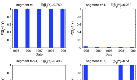
   Figure 2: Five-year time series of the posterior probabilities $P(s_{t,n}=1|{\bf Y})$ of the normal-count state $s_{t,n}=1$ for four selected roadway segments ($t=1,2,3,4,5$).

3. For roadway segments from the third category $P(s_{t,n}=1|{\bf Y})$ is neither one nor close to zero for all $t=1,2,3,4,5$. For these segments we cannot determine with high certainty what states these segments were in during years $t=1,2,3,4,5$. A roadway segment $n$ belongs to this category if it had no any accidents observed over the considered five-year time interval and the accident rates were not large, $\lambda_{t,n}\lesssim 1$ for all $t=1,2,3,4,5$. In fact, when $\lambda_{t,n}\ll 1$, the posterior probabilities of the two states are close to one-half, $P(s_{t,n}=1|{\bf Y})\approx P(s_{t,n}=0|{\bf Y})\approx 0.5$, and no inference about the value of the state variable $s_{t,n}$ can be made. In this case of small accident frequencies, the observation of zero accidents is perfectly consistent with both states $s_{t,n}=0$ and $s_{t,n}=1$. An example of a roadway segment from the third category is given in the bottom-left plot in Figure 2. For this segment $E({\bar{p}}_{1}|Y)=0.496$ is about one-half.

4. Finally, the fourth category is a mixture of the three categories described above. Roadway segments from this fourth category have posterior probabilities $P(s_{t,n}=1|{\bf Y})$ that change in time between the three possibilities given above. In particular, for some roadway segments we can say with high certainty that they changed their states in time from the zero-accident state $s_{t,n}=0$ to the normal-count state $s_{t,n}=1$ or vice versa. An example of a roadway segment from the fourth category is given in the bottom-right plot in Figure 2. For this segment $E({\bar{p}}_{1}|Y)=0.510$ is about one-half. Thus we find a direct empirical evidence that some roadway segments do change their states over time.

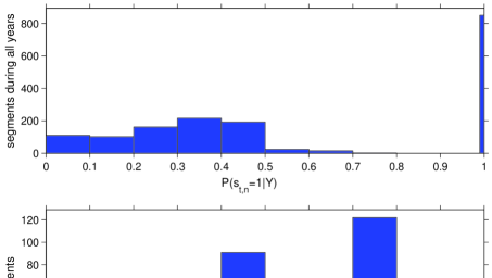
Figure 3: Histograms of the posterior probabilities $P(s_{t,n}=1|{\bf Y})$ (the top plot) and of the posterior expectations $E[\bar{p}^{(n)}_{1}|{\bf Y}]$ (the bottom plot). Here $t=1,2,3,4,5$ and $n=1,2,\ldots,335$.

Next, it is useful to consider roadway segment statistics by state of roadway safety. Referring to Figure 3, a case is made for the MSNB model. The top plot in this figure shows the histogram of the posterior probabilities $P(s_{t,n}=1|{\bf Y})$ for all $N=335$ roadway segments during all $T=5$ years ($1675$ values of $s_{t,n}$ in total). For example, we find that during five years roadway segments had $P(s_{t,n}=1|{\bf Y})=1$ and were normal-count in $851$ cases, and they had $P(s_{t,n}=1|{\bf Y})<0.2$ and were likely to be zero-accident in $212$ cases. The bottom plot in Figure 3 shows the histogram of the posterior expectations $E[\bar{p}^{(n)}_{1}|{\bf Y}]$, where $\bar{p}^{(n)}_{1}=p^{(n)}_{0\rightarrow 1}/(p^{(n)}_{0\rightarrow 1}+p^{(n)}_{1\rightarrow 0})$ are the stationary unconditional probabilities of the normal-count state (see Section 2). We find that $0.2\leq E[\bar{p}^{(n)}_{1}|{\bf Y}]\leq 0.8$ for all segments $n=1,2,\ldots,335$. This means that in the long run, all roadway segments have significant probabilities of visiting both the zero-accident and the normal-count states.

Finally, it is also worth mentioning that, in addition to negative binomial models, we estimated Poisson models for the same accident data and obtained similar results (Malyshkina, 2008). In particular, we found that a two-state Markov switching Poisson (MSP) model, which has the Poisson likelihood function instead of the NB likelihood function in Eq. (6), is strongly favored by the empirical data as compared to standard zero-inflated Poisson models.

5 Conclusions

A number of important observations can be made with regard to our empirical findings. First, Markov switching count-data models provide a superior statistical fit for accident frequencies relative to standard zero-inflated models. Second, Markov switching models, which explicitly consider transitions between the zero-accident state and the normal-count state over time, permit a direct empirical estimation of what states roadway segments are in at different time periods. In particular, we found evidence that some roadway segments changed their states over time (see the bottom-right plot in Figure 2). Third, note that the Markov switching models avoid a theoretically implausible assumption that some roadway segments are always zero-accident because, in these models, every segment has a non-zero probability of being in the normal-count state. Indeed, the long-term unconditional mean of the accident rate for the $n^{\rm th}$ roadway segment is equal to $\bar{p}^{(n)}_{1}\langle\lambda_{t,n}\rangle_{t}$, where $\bar{p}^{(n)}_{1}=p^{(n)}_{0\rightarrow 1}/(p^{(n)}_{0\rightarrow 1}+p^{(n)}_{1\rightarrow 0})$ is the stationary probability of being in the normal-count state $s_{t,n}=1$ and $\langle\lambda_{t,n}\rangle_{t}$ is the time average of the accident rate in the normal-count state [refer to Eq. (7)]. This long-term mean is always above zero (see the bottom plot in Figure 3), even for segments that were likely to be in the zero-accident state over the whole observed five-year time interval. Finally, we conclude that two-state Markov switching count-data models are likely to be a better alternative to zero-inflated models, in order to account for excess of zeros observed in accident-frequency data.

References

- Bohning et al. (1999) Bohning, D., Dietz, E., Schlattmann, P., Mendonca L., Kirchner, U., 1999: The zero-inflated Poisson model and the decayed, missing and filled teeth index in dental epidemiology. Journal of Royal Statistical Society A 162(2), 195 209.
- Broek (1995) van den Broek, J., 1995: A score test for zero-inflation in a Poisson distribution. Biometrics 51(2), 738 743
- Carson and Mannering (2001) Carson, J., Mannering, F. L., 2001. The effect of ice warning signs on ice-accident frequencies and severities. Accid. Anal. Prev. 33(1), 99-109.
- Cowan (1998) Cowan, G., 1998. Statistical Data Analysis. Clarendon Press, Oxford Univ. Press, USA
- Kass and Raftery (1995) Kass, R. E., Raftery, A. E., 1995. Bayes Factors. J. Americ. Statist. Assoc. 90(430), 773-795.
- Lambert (1992) Lambert, D., 1992: Zero-inflated Poisson regression, with an application to defects in manufacturing. Technometrics 34(1), 1 14.
- Lee and Mannering (2002) Lee, J., Mannering, F. L., 2002. Impact of roadside features on the frequency and severity of run-off-roadway accidents: an empirical analysis. Accid. Anal. Prev. 34(2), 149-161.
- Lord et al. (2005) Lord, D., Washington, S., Ivan, J. N., 2005. Poisson, Poisson-gamma and zero-inflated regression models of motor vehicle crashes: balancing statistical fit and theory. Accid. Anal. Prev. 37(1), 35-46.
- Lord et al. (2007) Lord, D., Washington, S., Ivan, J. N., 2007. Further notes on the application of zero-inflated models in highway safety. Accid. Anal. Prev. 39(1), 53-57.
- Maher and Summersgill (1996) Maher M. J., Summersgill, I., 1996. A comprehensive methodology for the fitting of predictive accident models. Accid. Anal. Prev. 28(3), 281-296.
- Malyshkina (2006) Malyshkina, N. V., 2006. Influence of speed limit on roadway safety in Indiana. MS thesis, Purdue University. http://arxiv.org/abs/0803.3436
- Malyshkina (2008) Malyshkina, N. V., 2008. Markov switching models: an application to roadway safety. PhD thesis in preparation, Purdue University. http://arxiv.org/abs/0808.1448
- Malyshkina et al. (2009) Malyshkina, N. V., Mannering, F. L., Tarko, A. P., 2009. Markov switching negative binomial models: an application to vehicle accident frequencies. Accid. Anal. Prev. 41(2), 217-226.
- Miaou (1994) Miaou, S. P., 1994. The relationship between truck accidents and geometric design of road sections: Poisson versus negative binomial regressions. Accid. Anal. Prev. 26(4), 471-482.
- Press et al. (2007) Press, W. H., Teukolsky, S. A., Vetterling, W. T., Flannery B. P., 2007. Numerical Recipes 3rd Edition: The Art of Scientific Computing. Cambridge Univ. Press, UK.
- Robert (2001) Robert, C. P., 2001. The Bayesian choice: from decision-theoretic foundations to computational implementation. Springer-Verlag, New York.
- Shankar et al. (1997) Shankar, V., Milton, J., Mannering, F., 1997. Modeling accident frequencies as zero-altered probability processes: an empirical inquiry. Accid. Anal. Prev. 29(6), 829-837.
- Spiegelhalter et al. (2002) Spiegelhalter, D. J., Best, N. G., Carlin, B. P., van der Linde, A., 2002. Bayesian measures of model complexity and fit. J. Royal Stat. Soc. B, 64, 583-639.
- Tsay (2002) Tsay, R. S., 2002. Analysis of financial time series: financial econometrics. John Wiley & Sons, Inc.
- Washington et al. (2003) Washington, S. P., Karlaftis, M. G., Mannering, F. L., 2003. Statistical and econometric methods for transportation data analysis. Chapman & Hall/CRC.
- Wood (2002) Wood, G. R., 2002. Generalised linear accident models and goodness of fit testing. Accid. Anal. Prev. 34, 417-427.