Emergence of zero-lag synchronization in generic mutually coupled chaotic systems

Abstract

Zero-lag synchronization (ZLS) is achieved in a very restricted mutually coupled chaotic systems, where the delays of the self-coupling and the mutual coupling are identical or fulfil some restricted ratios. Using a set of multiple self-feedbacks we demonstrate both analytically and numerically that ZLS is achieved for a wide range of mutual delays. It indicates that ZLS can be achieved without the knowledge of the mutual distance between the communicating partners and has an important implication in the possible use of ZLS in communications networks as well as in the understanding of the emergence of such synchronization in the neuronal activities.

Two identical chaotic systems starting from almost identical initial states, end in completely uncorrelated trajectories1 ; 1a . On the other hand, chaotic systems which are mutually coupled by some of their internal variables often synchronize to a collective dynamical behavior2 ; 3 . The emergence of synchronization plays important functioning roles in natural and artificial coupled systems. One of the most fascinating collective dynamical behavior is the zero-lag synchronization (ZLS), known also as an isochronal synchronization. ZLS or nearly ZLS was measured in the activity of the brain between widely separated cortical regions4a ; 5a ; 6a , where synchronization of neural activity has been shown to underlie cognitive acts3a . The mechanism of the ZLS phenomenon has been subject of controversial debate, where the main puzzle is how two or more distant dynamical elements can synchronize at zero-lag even in the presence of non-negligible delays in the transfer of information between them.

The phenomenon of ZLS was also experimentally observed in the synchronization of two mutually chaotic semiconductor lasers, where the optical path between the lasers is a few orders of magnitude greater than the coherence length of the laserseinat1 ; phase_sync ; ingo1 ; shutter , and the analogy between the spiking optical pattern and the neuronal spiking was also recently establishedspiking . This phenomenon has attracted a lot of attention, mainly because of its potential for secure communication over a public channeleinat1 . In hilbert it was recently shown that it is possible to use the ZLS phenomenon of two mutually coupled symmetric chaotic systems for a novel key-exchange protocol generated over a public-channel. Note that in contrary to a public scheme which is based on mutual coupling, private-key secure communication is based on a unidirectional couplingRoy ; nature and it is susceptible to an attacker which has identical parameters and is coupled to the transmitted signal. The generation of secure communication over a public channel requires mutual coupling and was only proven to be secure based on the ZLS phenomenonhilbert .

Recently, it has been shown both numerically and analytically that various architectures of coupled chaotic maps can exhibit ZLS7a ; sub_lat1 . The main disadvantage of this phenomenon is that ZLS even between two mutually coupled chaotic systems can be achieved only for very restricted architectures and it is highly sensitive for mismatch between the delays of the mutual coupling and the self-feedback. These delays have to be identical or have to fulfil special ratios. Such a realization might exist in a time-independent point-to-point communication, but it is far from the realm of communications networks.

In this letter we first demonstrate the constraint that ZLS is achieved only for very restricted ratios between the self-feedback and the mutual delays, $n\tau_{d}=m\tau_{c}$, where $n$ and $m$ are (small) integers. We next show that one can overcome this constraint when multiple self-feedbacks are used. For the simplicity of the presentation we mainly concentrate on the Bernoulli map, where results of simulations can be compared to an analytical solutionphysica_d ; sub_lat1 . However we observed the reported phenomenon for other chaotic maps and systems as well, and it is exemplified by the ZLS of mutually couple chaotic semiconductor lasers, depicted by the Lang-Kobayashi differential equationsLK ; einat1 .

The cornerstone of our system is the simplest chaotic map, the Bernoulli map, $f(x)=(ax)mod1$, which is chaotic for $a>1$. The dynamical equations of the two mutually coupled chaotic units, $X$ and $Y$, with one self-feedback (see solid lines in figure 1) are given by

$$\begin{split}\!\!\!\!x_{t}=(1-\varepsilon)f(x_{t-1})+\varepsilon[\kappa f(x_{t-\tau_{d}})+(1-\kappa)f(y_{t-\tau_{c}})]\\ \!\!\!\!y_{t}=(1-\varepsilon)f(y_{t-1})+\varepsilon[\kappa f(y_{t-\tau_{d}})+(1-\kappa)f(y_{t-\tau{c}})]\end{split}$$ (1)

where $\tau_{d}$ and $\tau_{c}$ are the delays of the self feedback and the mutual coupling, respectivelysub_lat1 . The quantities $1-\varepsilon$, $\varepsilon\kappa$ and $(1-\kappa)\varepsilon$ stand for the strength of the internal dynamics, self-feedback and the mutual coupling, respectively.

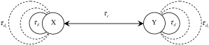
Figure 1: A schematic diagram of two mutually coupled units at a distance $\tau_{c}$ with one self-feedback with a delay equals to $\tau_{d}$ (solid lines). Additional self-feedbacks are denoted by the dashed lines.

The stationary solution of the relative distance between the trajectories of the two mutually coupled chaotic Bernoulli maps can be analytically examinedphysica_d ; sub_lat1 . Let us denote by $\delta x_{t}$ and $\delta y_{t}$ small perturbations from the trajectories $x_{t}$ and $y_{t}$, respectively. Using the ansatz $\delta x_{t}=c^{t}\delta x_{0}$ and $\delta y_{t}=c^{t}\delta y_{0}$ and linearizing equations (1), one can find the characteristic polynomial

$$\!\!\!\!c-a(1-\varepsilon)-a\varepsilon\kappa c^{1-\tau_{d}}+a\varepsilon(1-\kappa)c^{1-\tau_{c}}=0$$ (2)

where $\lambda=ln|c|$ is the Lyapunov exponent. Simulations of the dynamical equations (1) and the semi-analytical calculation of the maximal Lyapunov exponent of the characteristic polynomial (2), indicate that ZLS is the stationary solution of the dynamics only when the delays of the self-feedback and the mutual coupling fulfil the constraint

$$n\tau_{d}+m\tau_{c}=0$$ (3)

where the available integers for $n,m\in\mathbb{Z}$ are functions of $\epsilon$ and $\kappa$. Results are exemplified in figure 2 for $\epsilon=0.9$ and $\kappa=0.8$ (left panel) and for $\epsilon=0.9$ and $\kappa=0.4$ (right panel). For the left panel, ZLS is achieved for the pairs $(m,n)=(-1,n)$ where $n=1,2,...,10$ and $(3,-1)$comment2 . For the right panel ZLS is achieved for the pairs $(-1,n)~{}n=1,...,4$, $(3,-1)$, $(5,-1)$, $(7,-1)$, $(3,-2$) and $(5,-2)$even . Those lines may have width, so the more accurate equation is $|n\tau_{d}-m\tau_{c}|\leq\delta$, where $\delta\thickapprox 2$.

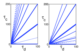
Figure 2: Simulations and semi-analytic results for the ZLS points in the phase space ($\tau_{d},\tau_{c}$) with $a=1.1,\varepsilon=0.9$ and $\kappa=0.8$ left panel and $\varepsilon=0.9$ and $\kappa=0.4$ right panel.

The constraint (3) indicates that ZLS can be achieved only when $\tau_{c}$ is accurately known, which is far from the realm of communications networks. In order to increase the possible ZLS range of $\tau_{c}$ for a fixed $\tau_{d}$, we added more self-feedbacks, as depicted in figure 1. The generalized dynamical equations for the case of multiple self-feedbacks are given by

$$x_{t}\!\!=\!\!(1-\varepsilon)f(x_{t-1})\!\!+\!\!\varepsilon[\kappa\sum_{l=1}^{N}\alpha_{l}f(x_{t-\tau_{d_{l}}})\!\!+\!\!(1-\kappa)f(y_{t-\tau_{c}})]$$

$$y_{t}\!\!=\!\!(1-\varepsilon)f(y_{t-1})\!\!+\!\!\varepsilon[\kappa\sum_{l=1}^{N}\alpha_{l}f(y_{t-\tau_{d_{l}}})\!\!+\!\!(1-\kappa)f(x_{t-\tau_{c}})]$$ (4)

where $N$ stands for the number of self-feedbacks and the parameter $\alpha_{l}$ indicates the weight of the $l^{th}$ self-feedback fulfilling the constraint $\sum_{l=1}^{N}\alpha_{l}=1$. In order to reveal the interplay between possible $\tau_{c}$ which lead to ZLS and a given set of $\{\tau_{d_{l}}\}$ we first examine in detail the case of $N=2$.

Results of simulations with $N=2$ which were confirmed by the calculation of the largest Lyapunov exponent obtained from the solution of the characteristic polynomial, similar to equation (2), are depicted in figure 3. The synchronization points $(\tau_{d_{1}},~{}\tau_{d_{2}})$ where ZLS is achieved form straight lines. A careful analysis of the equations of these lines indicates that their equations are

$$n_{1}\tau_{d_{1}}+n_{2}\tau_{d_{2}}+m\tau_{c}=0$$ (5)

where $n_{1},n_{2}$ and $m$ are integers. The lines may have a small width, hence a more accurate equation for the ZLS points is $|n_{1}\tau_{d_{1}}+n_{2}\tau_{d_{2}}+m\tau_{c}|\leq\delta$, where $\delta\thickapprox 2$. The same equations for the ZLS lines and with similar possible width, $\delta$, were obtained in simulations with different $\epsilon,~{}\kappa,~{}\alpha_{i}$ and $\tau_{c}$, prime and non-prime numbers in the range $[31,720]$.

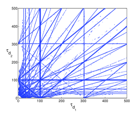
Figure 3: Simulations and semi-analytic results for the ZLS points in the phase space ($\tau_{d_{1}},\tau_{d_{2}}$) for $\tau_{c}=101,~{}a=1.1,\varepsilon=0.9$, $\kappa=0.8$ and $\alpha_{i}=1/2$.

Figure 3 indicates that for $\epsilon=0.9$ and $\kappa=0.8$comment3 , for instance, $m$ can take the integers $\pm 1$ and $\pm 3$ only. In order to examine the possible range of the integers $\{n_{i}\}$ we ran an exhaustive search simulation, $-6\leq n_{i}\leq 6$ and $m=\pm 1,~{}\pm 3$, and obtained integer $\tau_{c}$ from equation (5). Figure 4 depicts results of such an exhaustive search and the analytical solution of appropriate characteristic polynomials. The comparison between the results indicates the following two main conclusions: (a) $n_{i}\thickapprox 6$ gives a similar synchronization range, (b) the lines have an extension of up to $2$, hence the actual ZLS points fulfil the equation $|n_{1}\tau_{d_{1}}+n_{2}\tau_{d_{2}}+m\tau_{c}|\leq 2$ (see the inset of figure 4). Note that a few blue points are missing in the ZLS obtained in the semi-analytical solution (red points) indicating that a few combinations $(n_{1},n_{2},m)$ are missing.

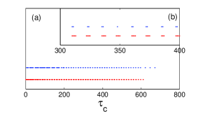
Figure 4: ZLS for two mutually coupled Bernoulli maps with $a=1.1,\varepsilon=0.9$ and $\kappa=0.8$ and with two self-feedbacks,$\tau_{d_{1}}=25,\tau_{d_{2}}=87$. ZLS points obtained from the exhaustive search of eq. (5) with $m=\pm 1,\pm 3$ and $n_{i}$ in the range $[-6,6]$ (blue points). The ZLS points obtained from simulation and semi-analytical results (red points). The inset is a blow up of a section of possible $\tau_{c}$ with ZLS.

We also analyze in detail the case of triple self-feedbacks, equation (4) with $N=3$, and find that ZLS points follow the equation $|n_{1}\tau_{d_{1}}+n_{2}\tau_{d_{2}}+n_{3}\tau_{d_{3}}+m\tau_{c}|\leq\delta\sim 2$, and in this case the ZLS points form planes.

The generalization of the ZLS points for $N=1,2$ and $3$ to the case of multiple self-feedbacks is

$$\sum_{i=1}^{N}n_{i}\tau_{d_{i}}+m\tau_{c}=0$$ (6)

where $n_{i}$ and $m$ take bounded integer values. This generalization was indeed confirmed in simulations and solving the characteristic polynomials with up to $N=7$.

In order to obtain a continuous range of $\tau_{c}$ for which ZLS is achieved, we examined the scenario of $4$ different $\tau_{d_{i}}=11,15,18,150$. We select one remarkably large $\tau_{d}$ such that we can see its effect on the range of $\tau_{c}$ where ZLS is achieved. To measure the quality of the ZLS we used the correlation function, which is defined by

$$C=\frac{\langle x_{t}y_{t}\rangle-\langle x_{t}\rangle\langle y_{t}\rangle}{\sqrt{\langle x^{2}_{t}\rangle-{\langle x_{t}\rangle}^{2}}\sqrt{\langle y^{2}_{t}\rangle-{\langle y_{t}\rangle}^{2}}}$$ (7)

where $C=1$ indicates complete ZLS and $\langle...\rangle$ stands for an average over the last $1000$ time steps. The correlation function, $C$, obtained in simulations is depicted in figure 5 and indicates the following results. Multiple self-feedbacks result in a continuous range of ZLS for $\tau_{c}$, hence it is not required to know exactly the mutual distance (value), $\tau_{c}$.

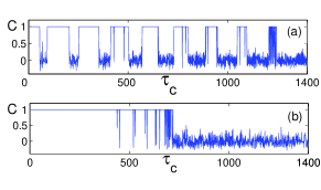
Figure 5: Simulations results of the correlation, $C$, as a function of $\tau_{c}$ for $a=1.1,\varepsilon=0.9$ and $\kappa=0.8$ and four $\tau_{d_{i}}=11,15,18,150$. The weight of the self-feedbacks, $\alpha_{i}$ in eq. (4), are in (a) $\alpha_{1}=\alpha_{2}=\alpha_{3}=0.25/3$ and $\alpha_{4}=0.75$ and in (b) $\alpha_{1}=\alpha_{2}=\alpha_{3}=0.65/3$ and $\alpha_{4}=0.35$

Panel (a) of figure 5 indicates that there are at least $7$ continuous ZLS regimes, each one of them is centered at $150n_{4}$, where $n_{4}=0,1,~{}...,~{}6$ and the plateaus are extended $\sim\pm 60$ around the centers (slightly decreases with increasing $n_{4}$). This width, $\pm 60$, is much smaller than the ZLS range of the only three short self-feedbacks $11,15,18$ which was found to be $\sim[1,150]$, indicating that the effective $n_{1},n_{2}$ and $n_{3}$ in eq. (6) are less than $6$. This discrepancy is a result of the dominated weight of $\tau_{4}=150$, $\alpha_{4}=0.75$, in figure 5(a). For a smaller weight for the largest delay $150$, $\alpha_{4}=0.35$, panel (b) of figure 5, a ZLS is continuously achieved up to $\tau_{c}\sim 700$. In this case a weak weight for the largest delay results in limited $n_{4}$ which takes the values of $0,1,2,3,4$ only, and we expect ZLS in four continuous regimes centered around $\tau_{c}=0,~{}150,~{}300,~{}450$ and $600$Anja . However these four regimes are now merged by the $\pm 150$ width inspired by the strengthened weight for the short self-feedbacks, $\alpha_{1}=\alpha_{2}=\alpha_{3}=0.65/3$comment1 .

In the general case there is an interplay between the following three parameters characterizing the set of the delay times: $\tau_{d_{max}}$ which is comparable to $\tau_{c}$, $\{\tau_{d_{i}}\}\ll\tau_{d_{max}}$ and $\Delta_{i}=\tau_{d_{i+1}}-\tau_{d_{i}}$ $i=1,...~{}N-2$, where $\{\tau_{d_{i}}\}$ are arranged in an increasing rank order. For instance, the following three sets of four self-feedbacks $(2,6,9,150),~{}(11,15,18,150),~{}(80,84,87,150)$ are characterized by the same $\tau_{d_{max}}$, $\Delta_{1}$ and $\Delta_{2}$. What is the main difference between the ZLS profile of these sets and which set maximizes the continuous range of ZLS? The first set opens only a small continuous ZLS regime ($\sim 20$ for parameters of panel (a)) around $150n_{4}$, since the time delays are very short. The third set almost does not open a continuous regime of ZLS, since $\tau_{d_{1}},\tau_{d_{2}},\tau_{d_{3}}\gg\Delta_{1},\Delta_{2}$. The maximal continuous ZLS range is achieved when short delays $\tau_{d_{1}},\tau_{d_{2}},\tau_{d_{3}}$ are comparable with $\sim 6\Delta_{1},6\Delta_{2}$ (see eq. (6)) which is a case of the second set.

Most of the reported simulations were carried out from close initial conditions, however, one can find $(\epsilon,\kappa)$ such that ZLS is achieved from random initial conditions at a comparable time to ZLS with only one time delay, $\tau_{c}\!=\!\tau_{d}$.

Similar results were obtained also for mutually coupled chaotic logistic maps where the Lyapunov exponent is fluctuating in time and is positive only on the average.

Finally we report that a similar phenomenon of ZLS occurs in simulations of two mutually coupled semiconductor lasers depicted by the Lang-Kobayashi equationsLK . Our simulations are based on the version and the parameters of these equations as in einat1 , with additional time delays. Figure 6(a) depicts the ZLS as a function of $\tau_{c}$ for the case of $4$ time delays $\tau_{d_{i}}=3,4,5,20ns$ and $\kappa_{i}=\sigma=30ns^{-1}$ and in figure 6(b) for $6$ time delays $\tau_{d_{i}}=11,12,13,14,15,16ns$ with $\kappa_{i}=\sigma=25ns^{-1}$, where for both cases the threshold current was $p=1.02$. For each $\tau_{c}$ the duration of the simulation was $7000ns$ and the emergence of ZLS was estimated from the measured cross correlation of the last $20$ windows of $100ns$comment . Results indicate that for the case of $6$ delays ZLS is achieved in the range $\sim[1,80]ns$ where for the case of $4$ time delays for $\sim[1,45]ns$shore . These synchronization regimes can be explained by equation (6) with $n_{i}=0,\pm 1,\pm 2$ only. It is consistent with our simulations of only one time delay where ZLS is achieved for $\tau_{d}=n\tau_{c}$ with $n=1,2,3$ only (instead of $1,...,~{}6$ for the examined maps) . Note that no extension on a time scale of $ns$ is expected, $\delta=0$, however, preliminary results indicate that a similar phenomenon occur where $\Delta_{i}=0.01ns$ which is comparable with the coherence length of the laser.

The research of I.K. is partially supported by the Israel Science Foundation.

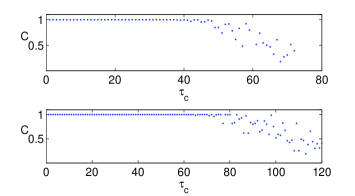
Figure 6: Simulation results of the correlation, eq. (7), for two mutually coupled semiconductor lasers (details in the text). Panel (a) for $4$ delays $\tau_{d}=3,4,5,20ns$ and panel (b) for $6$ time delays  $\tau_{d},=11,12,13,14,15,16ns$.

References

- (1) H. G. Schuster, W. Just. Deterministic Chaos. Wiley VCH, (2005).
- (2) S. Boccaletti, J. Kurths, G. Osipov, D. L. Valladares, and C. S. Zhou, Phys. Rep. 366, 1 (2002).
- (3) A. Pikovsky, M. Rosenblum, J. Kurths. Synchronization: A Universal Concept in Nonlinear Sciences, Cambridge Univ. Press, N.Y. (2001).
- (4) L. M. Pecora, T. L. Carroll, Phys. Rev. Lett. 64, 821 (1990).
- (5) A. K. Engel, P. Ko nig, A. K. Kreiter, and W. Singer, Science 252, 1177 (1991).
- (6) P. R. Roelfsema, A. K. Engel, P. Ko nig, and W. Singer, Nature (London) 385, 157 (1997).
- (7) G. Schneider and D. Nikolic, J. Neurosci. Methods 152 , 97 (2006).
- (8) E. Rodriguez, N. George, J.-P. Lachaux, J. Martinerie, B. Renault, and F. J. Varela, Nature (London) 397, 430 (1999).
- (9) E. Klein, N. Gross, E. Kopelowitz, M. Rosenbluh, L. Khaykovich, W. Kinzel, and I. Kanter, Phys. Rev. E 74, 046201 (2006)
- (10) Y. Aviad, I. Reidler, W. Kinzel, I. Kanter, and M. Rosenbluh, Phys. Rev. E 78, 025204 (2008).
- (11) I. Fischer, R. Vicente, J. M. Buldu, M. Peil, C. R. Mirasso, M. C. Torrent and J. G. Carciaa-Ojalvo, Phys. Rev. Lett. 97, 123902 (2006).
- (12) I. Kanter, N. Gross, E. Klein, E. Kopelowitz, P, Yoskovits, L. Khaykovich, W. Kinzel and M. Rosenbluh, Phys. Rev. Lett. 98, 154101 (2007).
- (13) M. Rosenbluh, Y. Aviad, E. Cohen, L. Khaykovich, W. Kinzel, E. Kopelowitz, P. Yoskovits and I. Kanter, Phys. Rev. E 76, 046207 (2007)
- (14) I. Kanter, E. Kopelowitz, and W. Kinzel, Phys. Rev. Lett. 101, 084102 (2008).
- (15) G. D. VanWiggeren, R. Roy, Science 279, 1198 (1998).
- (16) A. Argyris et. al. Nature 438, 343 (2005).
- (17) F. M. Atay, J. Jost and A. Wende, Phys. Rev. Lett. 92, 144101 (2004).
- (18) J. Kestler, E. Kopelowitz, I. Kanter, and W. Kinzel, Phys. Rev. E 77, 046209 (2008)
- (19) S. Lepri and G. Giacomelli and A. Politi and F. T. Arecchi, Physica D 70, 235 (1993).
- (20) R. Lang, and K. Kobayashi, IEEE J. Quantum Electron. QE-16, 347 (1980).
- (21) For , ZLS is achieved independent of due to the interernal dynamics, see eq. (1).
- (22) Even integers appear, for instance, for , where ZLS is achieved for and . The range of also increase in the limit of weak chaos .
- (23) Note that the effective weight of the mutual coupling is but the weight of the self-feedback is . Hence, the ZLS is not expected to be equal to either panels of figure 2.
- (24) One can find analytically an upper bound for which for and , for instance, is ,which is consistent with our results.
- (25) The semi-analytical solution indicates that plateaus of ZLS are slightly wider and no few sudden drops among the plateaus. These tiny mismatches are due to almost zero maximal Lyapunov exponent close to the plateaus boundaries, and limited number of steps in simulations.
- (26) For threshold current , chaotic signals consnist of low frequency fluctuations (LFFs) where short desynchronizations occur with the used numerical integration , see also einat1 . We avoid this affect by calculating the average cross correlation (eq. 7) of the maximal among last windows of size each.
- (27) Our results are in disagreement with E. M. Shahverdiev and K. A. Shore, Phys. Rev. E 77, 057201 (2008)