THE EFFECT OF RANDOM SURFACE INHOMOGENEITIES ON MICRORESONATOR SPECTRAL PROPERTIES:
THEORY AND MODELING AT MILLIMETER WAVE RANGE

Abstract

The influence of random surface inhomogeneities on spectral properties of open microresonators is studied both theoretically and experimentally. To solve the equations governing the dynamics of electromagnetic fields the method of eigen-mode separation is applied previously developed with reference to inhomogeneous systems subject to arbitrary external static potential. We prove theoretically that it is the gradient mechanism of wave-surface scattering which is the highly responsible for non-dissipative loss in the resonator. The influence of side-boundary inhomogeneities on the resonator spectrum is shown to be described in terms of effective renormalization of mode wave numbers jointly with azimuth indices in the characteristic equation. To study experimentally the effect of inhomogeneities on the resonator spectrum, the method of modeling in the millimeter wave range is applied. As a model object we use dielectric disc resonator (DDR) fitted with external inhomogeneities randomly arranged at its side boundary. Experimental results show good agreement with theoretical predictions as regards the predominance of the gradient scattering mechanism. It is shown theoretically and confirmed in the experiment that TM oscillations in the DDR are less affected by surface inhomogeneities than TE oscillations with the same azimuth indices. The DDR model chosen for our study as well as characteristic equations obtained thereupon enable one to calculate both the eigen-frequencies and the Q-factors of resonance spectral lines to fairly good accuracy. The results of calculations agree well with obtained experimental data.

I Introduction

Nowadays microresonators (disk-, ring-, and spherical-shaped) evoke considerable interest because new possibilities have recently opened up to develop these types of resonators in the optical frequency range and to utilize them as oscillation systems for optical lasers bib:Polman04 . When used in lasers, such oscillation systems offer a number of serious advantages, among which are low-threshold currents, a high quality of the radiation spectrum, etc. Microresonators manufactured as a dielectric disk whose diameter is large as compared to the wave length of the radiation are nothing else but the open quasi-optical dielectric disk resonators which have long been known in the resonator technology for their potential to effectively sustain the electromagnetic (EM) field inside the resonator volume. The retention of the field is provided due to the total internal reflection (TIR) from the resonator side boundaries of waves making up resonance oscillations. As a result, EM oscillations of whispering gallery (WG) type arise. As far as their excitation is not accompanied by the additional dissipative loss, superhigh quality factors are achieved in the DDRs. Specifically, in laser systems, in spite of DDR’s microscopic dimensions (the disk diameter is normally about a few $\mu$m large), the quality factors can reach the order of $10^{8}$ and even more bib:Vahala03 .

The high quality factors of the DDRs, that are often prepared from doped silicon, are generally provided not only due to extremely small loss attainable in this material but also governed by resonator geometry and the perfection of the crystal it is made of. With a certain number of inhomogeneities (local and/or non-local, random and/or regular) in the resonator material, the ray picture of EM fields in the resonator changes dramatically as against its perfectly homogeneous counterpart. The inhomogeneities give rise to local violation of TIR conditions and in this way result in additional energy loss which is evident in the quality factor drop. From the above said there arises the problem of studying the effect produced by random inhomogeneities in the DDRs on their spectral characteristics.

In the theoretic analysis of the radiation loss of the DDR two types of inhomogeneities are normally distinguished. To the first type the inhomogeneities of volume nature belong, which are related to regular or random spatial variations of the permittivity in the bulk of the material the DDR is made of. The other class of inhomogeneities includes the so called “surface” imperfections normally related to the deviation of the DDR shape from the ideal cylindrical one. The influence of bulk random inhomogeneities on the resonance spectrum was previously studied by the present authors in the particular case of cavity resonators filled with randomly distributed dielectric particles bib:GanErTar07 . It was found that the physical mechanism through which inhomogeneities affect resonator spectrum is basically the intermode scattering. In the case of quasi-optical cavity resonator the peculiar feature of this type of scattering is the selective impact of inhomogeneities on different resonance lines. The most affected lines appear to be those which are the least separated on the frequency axis, whereas solitary lines are subjected to much lesser influence. Owing to such a selective effect of random inhomogeneities, the originally dense spectrum of the quasi-optical cavity resonator is considerably rarefied.

In Refs. bib:Little97 ; bib:Gorod00 ; bib:Oraevsk2002 ; bib:Borselli2004 , the investigations were undertaken into the impact of surface inhomogeneities on spectral properties of open dielectric resonators of cylindrical and spherical shape. The influence of boundary roughness upon the resonance lines was described by means of the simplified quasi-geometric approach where EM oscillations scattering due to edge inhomogeneities is taken into account by incorporating into the wave equation the fictitious polarization currents (PC) randomly distributed in space bib:Kuznetsov83 . In particular, within the framework of the model adopted in Ref. bib:Little97 the electromagnetic fields close to the resonator side surface were considered as being excited by randomly distributed near-surface current sources whose physical parameters were phenomenologically expressed through statistical characteristics of boundary asperities. It was precisely the radiation produced by these sources that led to the radiation loss of the resonator and, consequently, to the quality factor reduction.

Such an essentially phenomenological approach to the description of the effect produced by the roughness of open resonator boundaries on its spectral properties cannot be reckoned as satisfactory. The volume current method suggested in Ref. bib:Kuznetsov83 , which formed the basis for the PC concept, is, to a large extent, rough and approximate. In this method, the radiation loss is most frequently calculated using Green function of the Helmholtz equation. The particular form of this function is normally chosen proceeding from the prospective solution of wave equation in the far wave zone. Meanwhile, the very notion of the far zone is poorly defined for multiple sources located around the periphery of the quasi-optical DDR we deal with in this particular work. Specifically, when deriving characteristic equations for open DDR eigen-frequencies, one needs to join EM field components exactly at the boundaries of the system under consideration. At this point a significant uncertainty can arise because the actual external fields subject to local joining with the internal ones in the presence of surface roughness can deviate considerably from the fields approximated into the boundary vicinity from large distances, i. e. from the far wave zone.

To correctly determine the EM fields near the random-inhomogeneous resonator surface the theories specially adapted for the description of classic and/or quantum wave scattering by rough interfaces should be applied (see, e. g., Refs. bib:BassFuks79 ; bib:Ogilvy91 ; bib:Voronovich94 ). These theories are generally applicable to the cases where wave scattering by random rough surfaces is in a sense weak. Typically, this implies fluctuations of system boundaries to be relatively small in height and sufficiently smooth, so that the applicability of Rayleigh hypothesis bib:Rayleigh1907 ; bib:Rayleigh45 was not violated. However, for confined systems like the DDR considered in this work the issues pertinent to wave scattering by surface inhomogeneities appear to be much more complicated. Firstly, in practice the inhomogeneities are not always small enough, as well as sufficiently smooth, therefore the conditions for scattering weakness are easily violated. Moreover, as the resonance ray trajectories in high-Q resonators are periodic, the effect of oscillation scattering caused by the boundary roughness is “path”-accumulated. Scattering can become strong even though the asperities are small-in-height and smooth. This makes the applicability of the above-mentioned theories of rough-surface scattering in the case of high-quality resonators highly questionable.

In Refs. bib:MakTar98 ; bib:MakTar01 , the novel transport theory was developed for waveguide-shaped systems with random rough boundaries. In the framework of this theory it was revealed that the wave scattering resulting from fluctuations of inter-media surfaces can be efficiently described in terms of two physical mechanisms, namely, the amplitude and the gradient ones. For the first mechanism it is just the mean-square height of the asperities that serves as a main guiding parameter, whereas for the second one the mean slope of the asperities or, in other words, their sharpness, plays the decisive role. Both of these mechanisms contribute additively to the scattering amplitude, but partial probabilities pertaining to them may differ essentially. It was shown in bib:MakTar98 ; bib:MakTar01 that, in most cases, the role of the gradient scattering appears to be prevalent. Yet there have been no experimental confirmations of this fact in the literature so far.

Apart from peculiar problems associated with surface nature of scattering in edge-disordered resonators, some more questions arise which need to be resolved when studying the spectra of DDRs subject to surface inhomogeneities. Among these questions, particularly, are those related to the vector nature of fields which are excited in these essentially non-integrable systems. It is known that even for ideal cylindrical DDRs the electrical- and magnetic-type oscillations cannot be separated in the strict sense. They always remain to the certain extent intermixed bib:Vainstein88 . This fact renders theoretic analysis of such systems spectra rather sophisticated. Spectral properties of DDRs without random inhomogeneities were examined in a number of theoretical papers (see, e. g., Refs. bib:IvanovKalin1988 ; bib:Peng96 ; bib:Anino97 ). Yet, in deriving characteristic equations some inexact a priori assumptions where used, which still require both theoretical grounding and experimental corroboration.

In our present study, one of the goals is to investigate theoretically the physical mechanisms responsible for widening resonance lines of dielectric microresonators with random surface inhomogeneities. In view of such systems being non-integrable, it is necessary to elaborate an appropriate theoretical model allowing for sufficiently accurate determination of both the frequency spectrum and the quality factors of resonance lines. Yet another goal of this study is to corroborate experimentally which of the physical mechanisms does play a dominant role in the scattering of EM oscillations excited in microresonators with random rough side boundaries.

From the theoretical viewpoint, the spectrum analysis in our study is carried out in terms of scalar potentials, specifically, electrical and magnetic Hertz functions bib:Vainstein88 . We formulate the conditions wherein these potentials make independent contributions to EM fields in the resonator, which is equivalent to decoupling the oscillations of TE and TM polarization. The Helmholtz equation for Hertz potentials in an irregular-shaped open resonator is equivalent to Schrödinger equation for electrons moving in the piecewise continuous space subject to random potential. Owing to this one can extend the results obtained in the present study to quantum systems as well, in particular, to open quantum dots having random rough boundaries.

To solve wave equations in the rough-bounded resonator, the eigen-mode separation method is used, previously developed with reference to waveguide-like systems subject to arbitrary static potential bib:Tar00 ; bib:Tar03 ; bib:Tar05 ). Using this method, the originally posed statistical problem of determining the fields in three-dimensional DDR with complex, randomly rough, side boundary is rigorously reduced to the set of one-dimensional dynamic equations that contain some effective random potentials. We show that under the conditions where gradient scattering mechanism is dominant, the boundary roughness effect on the resonator spectrum can be described through certain renormalization of mode wave numbers and azimuth indices of the Bessel functions in the characteristic equation. The values of renormalized wave numbers and mode indices decrease as the asperities get sharpened, which is consistent with a decrease in the resonator Q-factor. We are thus led to the conclusion that the observed reduction of resonant line quality factors results not from the extra dissipative loss but rather from EM field intermode Rayleigh scattering induced by random surface inhomogeneities. The imperfection of the resonator shape results in the local violation of the TIR conditions. This leads to additional radiation loss of EM energy and, hence, to a decrease in the level of localization of EM fields inside the resonator.

Since characteristic dimensions of surface inhomogeneities in actual microresonators are always quite small (of the order of nanometers), to verify our theoretical findings experimentally we have decided upon the method of simulation with macroscopic devices. As a model system we have employed a millimeter wave quasi-optical resonator made of a circular teflon disk. WG oscillations of TE and TM types were excited in the disk using a special waveguide antenna. The inhomogeneities of the resonator side boundary were made in the form of teflon bracket-bars randomly attached to the outside cylindrical surface. Our experimental results have demonstrated excellent qualitative agreement with the developed theory as regards spectral lines widening caused by the resonator side boundary roughness. Furthermore, the relatively simple model of the DDR field distribution, which was adopted in our study, enabled us to calculate both the Q-factors and the frequencies of the resonance lines with quite satisfactory accuracy. The calculations appeared to be in fair conformity with our experimental data.

II Theoretical model and derivation of basic equations

Consider an open disk resonator as a finite-height cylinder made of the dielectric material with permittivity $\varepsilon_{0}$. Plain-parallel end boundaries of the cylinder traverse the central axis ($z$) at points $z_{\pm}=\pm H/2$ (see Fig. 1), the side boundary ($S$) is formed by the generatrix passing parallel to $z$-axis along closed contour $C$

.8in

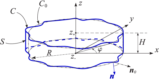
Figure 1: (Color online) The sketch of the dielectric cylindrical resonator with a randomly rough side wall. Vectors $\mathbf{n}$ and $\mathbf{n_{0}}$ point out the local normal directions to the rough ($S$) and to the smoothed resonator side surface, respectively.

whose distance from the central axis is given by

$$r(\varphi)=R+\xi(\varphi)\ ,\qquad\qquad\varphi\in[-\pi,\pi]\ ,$$ (1)

$R$ is the radius of the averaged (i. e., ideally circular) contour $C_{0}$ containing no random bends. The function $\xi(\varphi)$ will be regarded as the Gaussian random process with a zero mean value, $\big{<}\xi(\varphi)\big{>}=0$, and binary correlation function

$$\big{<}\xi(\varphi)\xi(\varphi^{\prime})\big{>}=\sigma^{2}W(\varphi-\varphi^{\prime})\ .$$ (2)

Here, $\sigma$ is the mean-square height of boundary asperities, $W(\varphi)$ is the dimensionless function which has a unit maximal value at zero argument and falls to parametrically small values at angle distance $\varphi_{c}\ll 1$ (the correlation angle). The angle brackets in Eq. (2) denote statistical averaging over the ensemble of realizations of random function $\xi(\varphi)$. In what follows, for the estimation purposes, along with angle parameter $\varphi_{c}$ we will use another correlation parameter, viz., arc correlation length $s_{c}=\varphi_{c}R$. Both the random function $\xi(\varphi)$ and the regular $W(\varphi)$ will be thought of as periodic with period $2\pi$.

It is well known that in general the EM field of an open dielectric resonator can be given as a superposition of oscillations of electric and magnetic types (TM and TE polarized, respectively) bib:Vainstein88 . The vector fields of both of these types can be expressed in terms of scalar potentials, $U(\mathbf{r})$ and $V(\mathbf{r})$ (the so-called electric and magnetic Debye potentials), which meet the same Helmholtz equation but are subject to different joining conditions at the resonator boundaries. In arbitrarily shaped resonators TM and TE oscillations are essentially intermixed, being strictly decoupled only in the case of sufficiently symmetric systems such as, e. g., an infinite dielectric cylinder bib:Vainstein88 or a dielectric sphere bib:Oraevsk2002 . Below it will be shown that TM and TE oscillations can also be decoupled (with high accuracy, though approximately) in the case of the cylindrical DDR of arbitrary thickness. This fact opens an opportunity to extend the conclusions of the present work to electronic microresonance systems, e. g., partially open quantum dots.

In studying oscillations in the DDR with randomly rough side boundaries we first reduce the problem of wave scattering at the boundary to the problem of scattering in the bulk of the resonator of ideal circular form. The Helmholtz equation for scalar wave field $\Psi(\mathbf{r})$, whose role is played by one of the above-mentioned potentials, after rewriting it in cylindrical coordinates and using the conformal coordinate transformation,

$$\widetilde{r} = \frac{r}{1+\xi(\varphi)/R}\ ,$$

$$\widetilde{\varphi} = \varphi\ ,$$ (3)

$$\widetilde{z} = z\ ,$$

is reduced to the form

$$\left[\frac{1}{r}\frac{\partial}{\partial r}r\frac{\partial}{\partial r}+\frac{1}{r^{2}}\frac{\partial^{2}}{\partial\varphi^{2}}+\frac{\partial^{2}}{\partial z^{2}}+K^{2}(r,z)-\hat{V}^{(h)}-\hat{V}^{(s)}\right]\Psi(r,\varphi,z)=0$$ (4)

(the tilde signs over coordinate variables from here on are omitted). Here, $K^{2}(r,z)=k^{2}\varepsilon(r,z)$,

$$\varepsilon(r,z)=\left\{\begin{array}[]{cl}\varepsilon_{0}+i/\tau_{0}&,\qquad(r,z)\in\Omega\\[6.0pt] 1&,\qquad(r,z)\not\in\Omega\end{array}\right.\ ,$$ (5)

$1/\tau_{0}$ is the phenomenological frequency parameter which takes into account dissipative and other uncontrollable losses in the system, except for the radiation loss, $\Omega$ is the bulk region occupied by the dielectric. Effective potentials $\hat{V}^{(h)}$ and $\hat{V}^{(s)}$ in Eq. (4) are the operators whose coordinate representation reads

$$\hat{V}^{(h)}=-\left[K^{2}(r,z)+\frac{\partial^{2}}{\partial z^{2}}\right]\left[\beta^{2}(\varphi)-1\right]\ ,$$ (6a)

$$\hat{V}^{(s)}=\left[\frac{\xi^{\prime}(\varphi)}{R\beta(\varphi)}\frac{\partial}{\partial\varphi}+\frac{\partial}{\partial\varphi}\frac{\xi^{\prime}(\varphi)}{R\beta(\varphi)}\right]\frac{1}{r}\frac{\partial}{\partial r}-\left[\frac{\xi^{\prime}(\varphi)}{R\beta(\varphi)}\right]^{2}\frac{1}{r}\frac{\partial}{\partial r}r\frac{\partial}{\partial r}\ ,$$ (6b)

$$\beta(\varphi)=1+\xi(\varphi)/R\ .$$

Indices “$h$” and “$s$” specifying potentials (6) indicate that the corresponding potential is mainly governed either by fluctuations in the asperity height (i. e. by height function $\xi(\varphi)$) or by fluctuations in the asperity slope (i. e., by slope function $\xi^{\prime}(\varphi)$). Such a subdivision of the potentials, with regard to the asymptotic suppression of correlations between functions $\xi(\varphi)$ and $\xi^{\prime}(\varphi)$ over angle intervals that are large as compared to the correlation angle, urges one to consider potentials (6a) and (6b) as corresponding to different physical wave-surface scattering mechanisms bib:MakTar98 ; bib:MakTar01 . We will below refer to these mechanisms as the amplitude (or the height, h) and the gradient (or the slope, s) scattering mechanisms, respectively.

Subsequently we will examine the boundary asperities which are sufficiently small in hight so as to meet inequality

$$\sigma\ll R\ .$$ (7)

In contrast to the widespread belief (see, e. g., Ref. bib:BassFuks79 ), this does not necessarily imply that the surface-roughness-induced scattering be regarded as weak. We note, for example, that the local value of the potential (6b) is estimated by the parameter $\sigma/s_{c}$, which may take an arbitrary absolute value provided the condition (7) is met. The true conditions for the scattering to be classified as weak will be provided below, based on the operator technique applied to perform the principal calculations.

III Separation of azimuth modes in randomly rough disk resonator

The potentials $\hat{V}^{(h)}$ and $\hat{V}^{(s)}$ in Eq. (4), that account for inhomogeneity of the resonator side-boundary, are defined not quite conveniently from the viewpoint of subsequent use of perturbation theories. The inconvenience relates to non-zero average value of the potential (6b). By separating this average, we can rewrite Eq. (4) as

$$\bigg{[}(1+\Xi^{2})\frac{1}{r}\frac{\partial}{\partial r}r\frac{\partial}{\partial r}+\frac{1}{r^{2}}\frac{\partial^{2}}{\partial\varphi^{2}}+\frac{\partial^{2}}{\partial z^{2}}+K^{2}(r,z)-\hat{V}^{(h)}-\hat{V}^{(s1)}-\hat{V}^{(s2)}\bigg{]}\psi(r,\varphi,z)=0\ ,$$ (8)

where two different slope potentials are introduced instead of potential Eq. (6b), which have zero mean values, viz.

$$\hat{V}^{(s1)}= \frac{1}{R}\left[\xi^{\prime}(\varphi)\frac{\partial}{\partial\varphi}+\frac{\partial}{\partial\varphi}\xi^{\prime}(\varphi)\right]\frac{1}{r}\frac{\partial}{\partial r}\ ,$$ (9a)

$$\hat{V}^{(s2)}= -\left[{\xi^{\prime}}^{2}(\varphi)/R^{2}-\Xi^{2}\right]\frac{1}{r}\frac{\partial}{\partial r}r\frac{\partial}{\partial r}\ .$$ (9b)

The parameter $\Xi$ in Eqs. (8) and (9b), which is defined as

$$\Xi^{2}=\frac{1}{R^{2}}\big{<}\left[\xi^{\prime}(\varphi)\right]^{2}\big{>}\sim\frac{\sigma^{2}}{s_{c}^{2}}\ ,$$ (10)

serves as a measure for the mean-square slope of boundary asperities.

Considering that irregularities of the resonator side surface are aligned paraxially, they cannot result in additional scattering along axis $z$ except for the partial reflection produced by the initial step change in this direction of the permittivity of the medium. This makes it possible to remove from Eq. (8) the dependence on the coordinate $z$ with the model method similar to the one we use when analyzing the spectrum of homogeneity-free DDR (see Appendix A). Specifically, we assume the dependence of the mode wave function on the coordinate $z$ to have the same form used to find $s$- and $a$-solutions for the ideal-shaped resonator (for the particular $E_{z}$-symmetric solution this dependence is given in Eqs. (36) and (37)). Afterwards, equation (8), being divided by the factor of $1+\Xi^{2}$, is reduced to the following form,

$$\bigg{[}\frac{1}{r}\frac{\partial}{\partial r}r\frac{\partial}{\partial r}+\frac{1}{(1+\Xi^{2})r^{2}}\frac{\partial^{2}}{\partial\varphi^{2}}+\widetilde{K}_{\bot}^{2}(r|z_{\scriptscriptstyle\lessgtr})-\widetilde{{V}}^{(h)}(z_{\scriptscriptstyle\lessgtr})-\widetilde{\hat{V}}^{(s1)}-\widetilde{\hat{V}}^{(s2)}\bigg{]}\Psi(r,\varphi|z_{\scriptscriptstyle\lessgtr})=0\ ,$$ (11)

where

$$\widetilde{K}_{\perp}^{2}(r|z_{\scriptscriptstyle\lessgtr}) =\frac{1}{1+\Xi^{2}}\left\{\begin{array}[]{clcl}\big{[}\varepsilon\theta(R-r)+\theta(r-R)\big{]}k^{2}-k_{z}^{2}&\ \text{,}&\qquad|z|&<H/2\\ k^{2}+\varkappa_{z}^{2}&\ \text{,}&\qquad|z|&>H/2\end{array}\ ,\right.$$ (12c)

$$\widetilde{{V}}^{(h)}(z_{\scriptscriptstyle\lessgtr}) =-\widetilde{K}_{\perp}^{2}(r|z_{\scriptscriptstyle\lessgtr})\left[\beta^{2}(\varphi)-1\right]\ .$$ (12d)

The tilde signs over the potentials in Eq. (11) denote their renormalization by the factor of $\big{(}1+\Xi^{2}\big{)}^{-1}$. Equation (11) actually describes two-dimensional fields because symbol $z_{\scriptscriptstyle\lessgtr}$ acts not as the current axial coordinate but stands for some axial index specifying in which domain of the $z$-axis — either $|z|<H/2$ or $|z|>H/2$ — the solution to Eq. (8) is sought.

In the azimuth mode representation, equation (11) assumes the form

$$\left[\frac{1}{r}\frac{\partial}{\partial r}r\frac{\partial}{\partial r}+\widetilde{K}_{\perp}^{2}(r|z_{\scriptscriptstyle\lessgtr})-\frac{\widetilde{n}^{2}}{r^{2}}-\widetilde{\mathcal{V}}_{n}(r|z_{\scriptscriptstyle\lessgtr})\right]\Psi_{n}(r|z_{\scriptscriptstyle\lessgtr})-\sum_{m\neq n}\widetilde{\mathcal{U}}_{nm}(r|z_{\scriptscriptstyle\lessgtr})\Psi_{m}(r|z_{\scriptscriptstyle\lessgtr})=0\ .$$ (13)

Here,

$$\widetilde{\mathcal{U}}_{nm}(r|z_{\scriptscriptstyle\lessgtr})=\oint d\varphi\bm{\langle}\varphi,n\bm{|}\widetilde{V}(r,\varphi|z_{\scriptscriptstyle\lessgtr})\bm{|}\varphi,m\bm{\rangle}\$$ (14)

is the matrix element of the entire potential $\widetilde{V}(r,\varphi|z_{\scriptscriptstyle\lessgtr})=\widetilde{{V}}^{(h)}(z_{\scriptscriptstyle\lessgtr})+\widetilde{\hat{V}}^{(s1)}+\widetilde{\hat{V}}^{(s2)}$, which is taken between eigen-functions of the azimuth part of the Laplace operator (see Appendix A), $\widetilde{\mathcal{V}}_{n}(r|z_{\scriptscriptstyle\lessgtr})\equiv\widetilde{\mathcal{U}}_{nn}(r|z_{\scriptscriptstyle\lessgtr})$, the index $n$ changes to ${\widetilde{n}=n\big{/}\sqrt{1+\Xi^{2}}}$. Later we will refer to matrix elements $\widetilde{\mathcal{V}}_{n}$ and $\widetilde{\mathcal{U}}_{nm}$ as the intra- and inter-mode potentials, respectively.

In the general case it is rather difficult to immediately solve the infinite set of coupled equations (13). However, the solution can be obtained in terms of the operator technique previously developed by the present authors with reference to waveguide-type random systems of arbitrary dimensionality bib:Tar00 ; bib:Tar03 and advantageously applied afterwards to the analysis of bulk-disordered cavity resonators bib:GanErTar07 . The above technique, as applied to the problem touched upon in the present paper, is adapted in Appendix B. The advantage of the technique is that it can be used to derive precise closed equations for wave functions of each of the azimuth modes, namely,

$$\left[\frac{1}{r}\frac{\partial}{\partial r}r\frac{\partial}{\partial r}+\widetilde{K}_{\perp}^{2}(r|z_{\scriptscriptstyle\lessgtr})-\frac{\widetilde{n}^{2}}{r^{2}}-\widetilde{\mathcal{V}}_{n}(r|z_{\scriptscriptstyle\lessgtr})-\hat{\mathcal{T}}_{n}\right]\Psi_{n}(r|z_{\scriptscriptstyle\lessgtr})=0\ .$$ (15)

Here, along with local intra-mode potential $\widetilde{\mathcal{V}}_{n}$, the operator potential $\hat{\mathcal{T}}_{n}$ arises, which rigorously allows for the inter-mode scattering. The structure of this potential, though well-recognized, is quite complicated to be operated with at an arbitrary scattering intensity. Yet, the estimations we provide in the next section substantially simplify the T-potential in Eq. (15) in different limiting cases, and in this way they allow one to obtain the oscillation spectrum of a randomly rough DDR in almost all physically sensible situations.

IV Spectrum of the DDR with weakly rough side boundary

Hereinafter we will refer to the system as weakly rough one if r.m.s. height of its boundary asperities meets inequality (7). As the potentials in Eq. (15) are of the operator nature, we will estimate their strength using standard definition of the operator norm bib:KolmFom68 ; bib:Kato66 . For our purposes the formula

$$\big{<}\big{\|}\hat{\mathsf{A}}\big{\|}^{2}\big{>}=\sup_{0\neq\psi\in\mathbb{X}}\frac{\big{<}(\hat{\mathsf{A}}\psi,\hat{\mathsf{A}}\psi)\big{>}}{(\psi,\psi)}$$ (16)

is the most appropriate, in which the parenthesis symbolize the scalar product on the functional space $\mathbb{X}$ consisting of the class of solutions to Eq. (15) with no random potentials.

To estimate the potentials in Eq. (11) we first calculate their azimuth matrix elements. For relatively small-height asperities the “height” potential ${\widetilde{V}}^{(h)}$ equals approximately ${\widetilde{V}}^{(h)}(z_{\scriptscriptstyle\lessgtr})\approx-2\widetilde{K}_{\perp}^{2}(r|z_{\scriptscriptstyle\lessgtr})\xi(\varphi)/R$. Mode matrix elements of this potential are

$$\widetilde{\mathcal{U}}_{nm}^{(h)}(r|z_{\scriptscriptstyle\lessgtr})=-\sqrt{\frac{2}{\pi}}\widetilde{K}_{\perp}^{2}(r|z_{\scriptscriptstyle\lessgtr})\frac{\widetilde{\xi}(n-m)}{R}\ ,$$ (17)

$\widetilde{\xi}(n)$ is the Fourier transform of the function $\xi(\varphi)$. Matrix elements of the “slope” potentials $\widetilde{\hat{V}}^{(s1)}$ and $\widetilde{\hat{V}}^{(s2)}$ are equal, respectively,

$$\widetilde{\mathcal{U}}_{nm}^{(s1)}(r)=-\frac{1}{\sqrt{2\pi}(1+\Xi^{2})R}\left(n^{2}-m^{2}\right)\widetilde{\xi}(n-m)\frac{1}{r}\frac{\partial}{\partial r}\ ,$$ (18a)

$$\widetilde{\mathcal{U}}_{nm}^{(s2)}(r)=\frac{1}{2\pi(1+\Xi^{2})R^{2}}\sum_{l=-\infty}^{\infty}(n-l)(l-m)\left[\widetilde{\xi}(n-l)\widetilde{\xi}(l-m)-\Big{<}\widetilde{\xi}(n-l)\widetilde{\xi}(l-m)\Big{>}\right]\frac{1}{r}\frac{\partial}{\partial r}r\frac{\partial}{\partial r}\ .$$ (18b)

IV.1 The efficiency of intra-mode scattering

We will ignore the role of the potential (17) for the intra-mode scattering proceeding from the following considerations. It is evident that under condition (7) the uniform azimuth mode of this potential can result, at most, in relatively small ($\sim\sigma/R$) renormalization of the unperturbed “in-plane energy” $\widetilde{K}_{\perp}^{2}(r|z)$. Yet, in the case we consider below even this does not occur. We will regard the asperities as not only being small in height but also as small-scaled ones in the sense that the inequality holds

$$s_{c}\ll R\quad\Longleftrightarrow\quad\varphi_{c}\ll 1\ .$$ (19)

In this limit the uniform mode of the random process $\xi(\varphi)$ with parametric accuracy ($\widetilde{\xi}(0)\sim\sigma\varphi_{c}$) can be put equal to zero, since the process is nearly ergodic within the interval of the angle variable change.

Gradient potential (18a) is not involved in the intra-mode scattering by its definition, so that only the potential (18b) should be taken into account, where one must let $m=n$. We use as trial functions in Eq. (16) the solutions of Eq. (15) with random potentials equal to zero, i. e., Bessel function $J_{\widetilde{n}}\big{[}\widetilde{K}_{\perp}(r|z_{\scriptscriptstyle\lessgtr})r\big{]}$ in the interval $0<r<R$ and Hankel function $H^{(1)}_{\widetilde{n}}\big{[}\widetilde{K}_{\perp}(r|z_{\scriptscriptstyle\lessgtr})r\big{]}$ in the domain $R<r<\infty$. Such a choice is justified provided the intra-mode scattering has a slight impact on the mode energies. Then we arrive at the following estimate for the potential $\widetilde{{\mathcal{V}}}_{n}$ norm,

$$\big{<}\big{\|}\widetilde{{\mathcal{V}}}_{n}\big{\|}^{2}\big{>}\sim\frac{\widetilde{K}_{\perp}^{4}}{(1+\Xi^{2})^{2}R^{4}}\Big{<}\bigg{[}\sum_{l=-\infty}^{\infty}l^{2}\Big{(}\big{|}\widetilde{\xi}(l)\big{|}^{2}-\big{<}\big{|}\widetilde{\xi}(l)\big{|}^{2}\big{>}\Big{)}\bigg{]}^{2}\Big{>}\ .$$ (20)

After averaging Eq. (20) using correlation equality

$$\big{<}\widetilde{\xi}(k)\widetilde{\xi}^{*}(l)\big{>}=\sqrt{2\pi}\sigma^{2}\widetilde{W}(k)\delta_{kl}\ ,$$ (21)

which immediately stems from Eq. (2) ($\widetilde{W}$ is the Fourier transform of correlation function $W(\varphi)$), we obtain

$$\big{<}\big{\|}\widetilde{{\mathcal{V}}}_{n}\big{\|}^{2}\big{>}\sim\frac{\widetilde{K}_{\perp}^{4}}{(1+\Xi^{2})^{2}}\left(\frac{\sigma}{R}\right)^{4}\sum_{l=-\infty}^{\infty}l^{4}\widetilde{W}^{2}(l)\approx\widetilde{K}_{\perp}^{4}\frac{\sigma}{R}\frac{\big{(}\sigma/s_{c}\big{)}^{3}}{\big{(}1+\sigma^{2}/s_{c}^{2}\big{)}^{2}}\ .$$ (22)

It can be readily seen that the factor standing at $\widetilde{K}_{\perp}^{4}$ in the right-hand side of Eq. (22) is, in view of Eq. (7), small as compared to unity. This substantiates the above assumption about the intra-mode scattering weakness.

IV.2 Comparative estimations of inter-mode potentials

The inter-mode scattering rate in our resonator is up to the norm of the operator $\hat{\mathsf{R}}$ entering T-matrix (54).

1. The “amplitude” inter-mode scattering.

When estimating the norm of the “height” item $\hat{\mathsf{R}}^{(h)}$ in the operator $\hat{\mathsf{R}}$ one is faced with a need to evaluate the expression

$$\big{<}\big{\|}\hat{\mathsf{R}}^{(h)}\big{\|}^{2}\big{>}\sim\frac{1}{\|\psi\|^{2}}\sum_{k}\int\limits_{0}^{\infty}rdr\sum_{m_{1},m_{2}\neq k}\int\limits_{0}^{\infty}r_{1}dr_{1}\int\limits_{0}^{\infty}r_{2}dr_{2}G^{(V)}_{k}(r,r_{1}){G^{(V)}_{k}}^{*}(r,r_{2})\Big{<}\widetilde{\mathcal{U}}_{km_{1}}^{(h)}(r_{1}){\widetilde{\mathcal{U}}_{km_{2}}^{(h)*}}(r_{2})\Big{>}\psi_{m_{1}}(r_{1})\psi_{m_{2}}^{*}(r_{2})$$ (23)

(in order not to overload subsequent formulae we omit axial index $z_{\scriptscriptstyle\lessgtr}$, as this cannot lead to misunderstanding; function $G^{(V)}_{k}(r,r_{1})$ is introduced in Appendix B). The simultaneous presence in Eq. (23) of both the integrals over radial coordinate $r$ and the sums over mode indices stems from the definition of the functional space where the operator $\hat{\mathsf{R}}$ is effective.

In view of Eqs. (17) and (21) the correlator in the integrand of Eq. (23) is calculated to

$$\Big{<}\widetilde{\mathcal{U}}_{km_{1}}^{(h)}(r_{1}){\widetilde{\mathcal{U}}_{km_{2}}^{(h)*}}(r_{2})\Big{>}=2\sqrt{\frac{2}{\pi}}\left(\frac{\sigma}{R}\right)^{2}\widetilde{K}^{2}_{\perp}(r_{1})\widetilde{K}^{2*}_{\perp}(r_{2})\widetilde{W}(k-m_{1})\delta_{m_{1}m_{2}}\ .$$ (24)

By substituting this into Eq. (23) and assuming the asperity correlation function to have the Gaussian form, viz. ${W(\varphi)=\exp\big{(}-\varphi^{2}/2\varphi_{c}^{2}\big{)}}$, we arrive at the following estimate for the height term in the inter-mode scattering operator,

$$\big{<}\big{\|}\hat{\mathsf{R}}^{(h)}\big{\|}^{2}\big{>}\sim(\widetilde{K}_{\perp}\sigma)^{2}\ .$$ (25)

The Rayleigh parameter $k\sigma$, to whose square the right-hand side of Eq. (25) is proportional, may take small or large values, depending upon the relationship between mean-square height of the asperities and the wave length of the excited oscillations. According to the value of this parameter we will distinguish between weak ($k\sigma\ll 1$) and strong ($k\sigma\gg 1$) inter-mode scattering caused by the “height” potential.

2. The “gradient” inter-mode scattering.

This type of scattering between different azimuth modes is related to the availability in Eq. (13) of the potentials (18). Their correlators needed to estimate the operator norms of items $\hat{\mathsf{R}}^{(s1)}$ and $\hat{\mathsf{R}}^{(s2)}$ in the operator $\hat{\mathsf{R}}$, are equal, respectively,

$$\Big{<}\widetilde{\mathcal{U}}_{km_{1}}^{(s1)}(r_{1}){\widetilde{\mathcal{U}}_{km_{2}}^{(s1)*}}(r_{2})\Big{>}= \frac{1}{\sqrt{2\pi}}\frac{\sigma^{2}}{(1+\Xi^{2})^{2}R^{2}}(k^{2}-m_{1}^{2})^{2}\widetilde{W}(k-m_{1})\delta_{m_{1}m_{2}}\frac{1}{r_{1}}\frac{\partial}{\partial r_{1}}\cdot\frac{1}{r_{2}}\frac{\partial}{\partial r_{2}}\ ,$$ (26a)

$$\Big{<}\widetilde{\mathcal{U}}_{km_{1}}^{(s2)}(r_{1}){\widetilde{\mathcal{U}}_{km_{2}}^{(s2)*}}(r_{2})\Big{>}= \frac{1}{(2\pi)^{2}(1+\Xi^{2})^{2}R^{4}}\left(\frac{1}{r_{1}}\frac{\partial}{\partial r_{1}}r_{1}\frac{\partial}{\partial r_{1}}\right)\left(\frac{1}{r_{2}}\frac{\partial}{\partial r_{2}}r_{2}\frac{\partial}{\partial r_{2}}\right)$$

$$\times\sum_{l_{1},l_{2}=-\infty}^{\infty}(k-l_{1})(l_{1}-m_{1})(k-l_{2})(l_{2}-m_{2})\Big{<}\widetilde{\xi}(k-l_{1})\widetilde{\xi}(l_{1}-m_{1})\widetilde{\xi}^{*}(k-l_{2})\widetilde{\xi}^{*}(l_{2}-m_{2})\Big{>}\ .$$ (26b)

Assuming the function $\xi(\varphi)$ to be the Gaussian random process, the equality (26b) can be partially simplified as the double sum over $l_{1}$ and $l_{2}$ is reduced to the single one,

$$\sum_{l_{1},l_{2}=-\infty}^{\infty}\ldots\ =4\pi\sigma^{4}\delta_{m_{1}m_{2}}\sum_{l=-\infty}^{\infty}(k-l)^{2}(l-m_{1})^{2}\widetilde{W}(k-l)\widetilde{W}(l-m_{1})\ .$$ (27)

Then the alternate substitution of correlation functions (26) into Eq. (23) in place of the height potential correlator results in the following estimation formulas for operators $\hat{\mathsf{R}}^{(s1)}$ and $\hat{\mathsf{R}}^{(s2)}$,

$$\big{<}\big{\|}\hat{\mathsf{R}}^{(s1)}\big{\|}^{2}\big{>} \sim\frac{\Xi^{2}}{(1+\Xi^{2})^{2}}\cdot\frac{1}{\varphi_{c}^{2}}\ ,$$ (28a)

$$\big{<}\big{\|}\hat{\mathsf{R}}^{(s2)}\big{\|}^{2}\big{>} \sim\left(\frac{\Xi^{2}}{1+\Xi^{2}}\right)^{2}(\widetilde{K}_{\perp}R)^{2}\ .$$ (28b)

The collation of norms (25) and (28) reveals that the height and the gradient scattering mechanisms, given their effect is evaluated as a function of roughness statistical parameters and radial components of the azimuth mode wave vectors, can essentially compete against one another. However, the general statement boils down to the fact that it is the gradient scattering which is prevalent in the most part of the parameter region. The amplitude scattering mechanism can also dominate, but this is the case for quite smooth asperities only and for oscillations of very large azimuth indices. One can conclude from Eqs.(25) and (28) that for the amplitude scattering to be dominant it is necessary, first, that the average tangent of the asperity angle of slope obey the condition

$$\overline{\tan\theta}\sim\frac{\sigma}{s_{c}}\ll\left(\frac{\sigma}{R}\right)^{1/2}\ .$$ (29a)

Secondly, the inequality must be fulfilled $$\left(K_{\perp}R\right)^{2}\gg\Xi^{2}\left(R/s_{c}\right)^{2}$$, which is admissible for oscillations with quite large mode indices, i. e.,

$$n\gg\left(\frac{R}{s_{c}}\right)^{2}\ .$$ (29b)

If only one of the inequalities (29) fails to hold (indeed, this is the case for the overwhelming majority of parameters from the above-mentioned set), the gradient scattering appears to be dominating.

IV.3 Whispering gallery modes of the rough-side DDR

Based on the above estimations, equation (15), that governs the azimuth mode spectrum of the resonance system under study can be substantially simplified if one considers the limiting cases of weak and strong scattering. As is seen from Eq. (22), for small r.m.s. height of the asperities (in the sense of inequality (7)) the intra-mode scattering due to potential $\widetilde{\mathcal{V}}_{n}$ is weak, thereby making it possible to disregard it in the main approximation.

As far as the inter-mode scattering is concerned, it is not straightforward to estimate it in the same way as the intra-mode one. From Eqs. (25) and (28) it follows that inter-mode scattering should be classified either as weak or strong one depending upon whether the operator $\hat{\mathsf{R}}$ norm is small or large as compared with unity. If the inter-mode scattering resulting from both the amplitude and the gradient potentials is thought of as weak one, which occurs when two inequalities hold simultaneously

$$k\sigma\ll 1\ ,$$ (30a)

$$\frac{\sigma}{s_{c}}\ll\frac{s_{c}}{R}\ ,$$ (30b)

the potential $\hat{\mathcal{T}}_{n}$ in Eq. (15) can be ignored with parametric accuracy. In this instance the resonator spectrum can be obtained from the equation which differs from the initial unperturbed one simply by renormalizing both the mode index ($n\to\widetilde{n}$) and the radial wave number ($K_{\perp}\to\widetilde{K}_{\perp}$). In the parameter region where both of the inequalities (30) are satisfied this renormalization is extremely small ($\Xi\ll\varphi_{c}$) and can be safely disregarded.

Conditions (30), that indicate the inter-mode scattering weakness, can be easily violated. By virtue of peculiar technology, when manufacturing micro- and nano-sized quantum resonance systems it is normally difficult to obey, e. g., inequality (30b) which corresponds to extreme smoothness of surface inhomogeneities. Moreover, inequality (30a) is fulfilled within only limited, i. e., long-wavelength, part of the resonator bandwidth.

If, at least, one of the conditions (30) is violated, the inter-mode scattering fails to be classified as a weak one in the sense that the norm of scattering operator $\hat{\mathsf{R}}$ in the potential (54) becomes large as against the unity. Nevertheless, in this case one may as well simplify the T-potential by expanding it in a series in the inverse scattering operator, $\hat{\mathsf{R}}^{-1}$. The expression between the projection operators in Eq. (54) is identically transformed as

$$\hat{\mathcal{U}}\left(\openone-\hat{\mathsf{R}}\right)^{-1}\hat{\mathsf{R}}= -\hat{\mathcal{U}}+\hat{\mathcal{U}}\left(\openone-\hat{\mathsf{R}}\right)^{-1}=-\hat{\mathcal{U}}-\hat{\mathcal{U}}\hat{\mathsf{R}}^{-1}\left(\openone-\hat{\mathsf{R}}^{-1}\right)^{-1}$$

$$= -\hat{\mathcal{U}}-\hat{\mathcal{U}}\,\hat{\mathcal{U}}^{-1}\hat{\mathcal{G}}^{(V)-1}\left(\openone-\hat{\mathsf{R}}^{-1}\right)^{-1}\approx-\hat{\mathcal{U}}-\hat{\mathcal{G}}^{(V)-1}-\hat{\mathcal{G}}^{(V)-1}\hat{\mathcal{U}}^{-1}\hat{\mathcal{G}}^{(V)-1}\ .$$ (31)

Here we use the symbolic notation $\hat{\mathcal{G}}^{(V)-1}$ for the full (i. e., including the whole set of azimuth modes) Green operator with no intermode potentials. As a result of “coating” Eq. (31) with the projection operators $\bm{P}_{n}$ the first term in its right-hand side is eliminated, and the operator acting on the wave function in Eq. (15) assumes the following approximate form,

$$\frac{1}{r}\frac{\partial}{\partial r}r\frac{\partial}{\partial r}+\widetilde{K}_{\perp}^{2}(r|z_{\scriptscriptstyle\lessgtr}) -\frac{\widetilde{n}^{2}}{r^{2}}-\widetilde{\mathcal{V}}_{n}(r|z_{\scriptscriptstyle\lessgtr})-\hat{\mathcal{T}}_{n}=\hat{G}_{n}^{(V)-1}-\hat{\mathcal{T}}_{n}$$

$$\approx 2\hat{G}_{n}^{(V)-1}+\bm{P}_{n}\hat{\mathcal{G}}^{(V)-1}\hat{\mathsf{R}}^{-1}\bm{P}_{n}\approx 2\left[\frac{1}{r}\frac{\partial}{\partial r}r\frac{\partial}{\partial r}+\widetilde{K}_{\perp}^{2}(r|z_{\scriptscriptstyle\lessgtr})-\frac{\widetilde{n}^{2}}{r^{2}}\right]\ .$$ (32)

By comparing the expression in the right-hand side of Eq. (32) with the one in its left-hand side, with potentials $\widetilde{\mathcal{V}}_{n}(r|z_{\scriptscriptstyle\lessgtr})$ and $\hat{\mathcal{T}}_{n}$ set to zero, one can notice that the limiting cases of weak and strong (in the sense of the operator $\hat{\mathsf{R}}$ norm) inter-mode scattering differ from one another solely by doubling the wave operator in the latter case. Clearly, such doubling implies that in strong surface scattering the amplitude of the excited oscillations is twice as small as the one in the weak scattering limit. However, it is evident that the change in the common factor multiplying the wave operator cannot reveal itself in dispersion relations.

We thus have demonstrated that the formal algebraic structure of the wave operator remains basically unchanged under conditions of weak and strong scattering. In both of these cases the wave operator differs slightly from its unperturbed form. The main difference between dispersion relations for resonators with perfect and rough side boundaries is that in the latter case the initial transverse wave parameter ${K}_{\perp}(r|z)$ and the mode index $n$ are renormalized by the gradient factor of $(1+\Xi^{2})^{-1/2}$. This enables us to immediately write down the dispersion equations for a DDR with random inhomogeneous side boundary based upon the results given in Appendix A. Specifically, for a rough-bounded DDR the oscillation spectrum is governed by the equation

$$\left[\frac{\varepsilon}{\widetilde{k}_{\perp}^{\varepsilon}}\cdot\frac{{J_{\widetilde{n}}}^{\prime}(\widetilde{k}_{\perp}^{\varepsilon}R)}{J_{\widetilde{n}}(\widetilde{k}_{\perp}^{\varepsilon}R)}-\frac{1}{\widetilde{k}_{\perp}}\cdot\frac{{H_{\widetilde{n}}^{(1)}}^{\prime}(\widetilde{k}_{\perp}R)}{H_{\widetilde{n}}^{(1)}(\widetilde{k}_{\perp}R)}\right]\Bigg{[}\frac{1}{\widetilde{k}_{\perp}^{\varepsilon}}\cdot\frac{{J_{\widetilde{n}}}^{\prime}(\widetilde{k}_{\perp}^{\varepsilon}R)}{J_{\widetilde{n}}(\widetilde{k}_{\perp}^{\varepsilon}R)}-\frac{1}{\widetilde{k}_{\perp}}\cdot\frac{{H_{\widetilde{n}}^{(1)}}^{\prime}(\widetilde{k}_{\perp}R)}{H_{\widetilde{n}}^{(1)}(\widetilde{k}_{\perp}R)}\Bigg{]}=\frac{\widetilde{n}^{2}}{R^{2}}(\varepsilon-1)^{2}\frac{k_{z}^{2}\widetilde{k}^{2}}{{(\widetilde{k}_{\perp}^{\varepsilon})}^{4}\widetilde{k}_{\perp}^{4}}\ ,$$ (33)

which has to be supplemented with additional relationships between $k$ and $k_{z}$, the latter resulting from joining the fields at the end interfaces. In Eq. (33), the notations are introduced $\big{(}\widetilde{n},\widetilde{k},\widetilde{k}_{\perp}^{\varepsilon},\widetilde{k}_{\perp}\big{)}=\big{(}n,k,k_{\perp}^{\varepsilon},k_{\perp}\big{)}\big{/}\sqrt{1+\Xi^{2}}$, the wave numbers $k_{\perp}^{\varepsilon}$ and $k_{\perp}$ are defined in Eq. (38).

As the additional connection between wave parameters $k$ and $k_{z}$ in the case of a perfect cylindrical resonator equation (43) is obtained for $E_{z}$-symmetric oscillations. For $E_{z}$-antisymmetric oscillations Eq. (44) holds. One can easily check that in going from unperturbed wave equation (35) to equation (8) describing the DDR with rough side wall the equations derived through joining EM field components at the end boundaries of the dielectric disk remain unchanged.

Finally, proceeding from the above calculations we are led to conclude that with any roughness of the DDR side wall, which is basically restricted by the smallness condition (7), to obtain the oscillation spectrum one can make use of the relationship Eq. (33) mainly coincident in form with the dispersion equation for an infinitely long dielectric cylinder. As a supplementary condition to interconnect the lengthwise and transverse wave vector components equation (43) or (44) should be applied, depending upon $E_{z}$-symmetry of the desired solution. The fundamental difference of Eq. (33) from its perfect-cylinder counterpart is the renormalization of basic wave parameters, which is governed by geometric properties of the asperities. A special emphasis should be placed on the fact that it is exactly the gradient scattering mechanism, not the amplitude one, that most crucially affects the DDR spectrum. This particular fact makes itself evident in that the renormalization of wave parameters in Eq. (33) is dictated not by the height-type parameters, such as, e. g., Rayleigh parameter $k\sigma$ or the ratio $\sigma/R$, but is mainly regulated by the mean-square slope of the asperities against the unperturbed resonator boundary, which is specified by parameter $\sigma/s_{c}$.

V Experimental results and discussion

The main goal of experimental studies in this work was to validate our theory as regards microresonator spectra and the effect of random surface inhomogeneities on them. The point is that essential assumption adopted in the theory is that it virtually does not consider electromagnetic fields radiated from the resonator external edges into the corner regions labeled by numbers 4 and 4^′ in Fig. 5 (see Appendix A). At the same time, without making quite complex calculations one cannot make a priori statements about these fields being small enough to neglect them in calculating the resonator spectrum. Yet another goal of the experiment was to examine our theoretical findings concerning the physical mechanism that adequately describes the influence of random surface inhomogeneities on microresonator spectral properties.

The studies of the microresonator spectrum were performed through modeling these quite small systems in the millimeter wave band. For this purpose we used a quasioptic dielectric disk resonator. Physically, oscillation properties of this macroscopic system are identical with properties of silicon microresonators used as oscillation systems in real optical lasers. Our resonator was made of teflon whose permittivity is not significantly far from unity ($\varepsilon=2.08$) and whose dielectric loss in the millimeter range are fairly small ($\tan\delta\cong 2.3\times 10^{-4}$). In the model DDR, whispering gallery oscillations were excited with the EM field concentrated at the periphery of the disk, in the narrow region close to its side boundary. This enabled us to use the disk core to fix it in the level position without introducing additional dissipative losses to the experiment. The source of WG modes was positioned close to the resonator side boundary. Its role was played by the waveguide antenna powered by the microwave generator. The antenna was fabricated as a waveguide tapered along the short wall, whose butt end was positioned near the resonator side surface. The receiving antenna was made identical to the source antenna and was placed at the diametrically opposite point off the disk.

Thin dielectric bracket-bars were used as the inhomogeneities of the resonator side boundary. They were attached to the DDR side surface. The basic requirement imposed on the inhomogeneities was for them not to cause noticeable additional dissipative losses. To this end, the bracket-bars

.8in

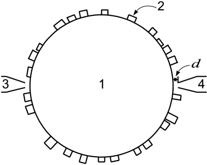
Figure 2: Schematic view of the experimental DDR with surface inhomogeneities: 1 — teflon disk; 2 — superimposed teflon bracket-bars (inhomogeneities); 3, 4 — the exciting and receiving waveguide antennas; $d$ — the gap between the antenna and the DDR’s side surface, which is used to tune the coupling of antenna with the resonator. The diameter of the DDR is 102 mm, the thickness is 7.6 mm. The inhomogeneities dimensions are: the length, the width, and the thickness 7.6 mm, 3 mm, and 2 mm, respectively.

were made of the same teflon as the resonator body. The inhomogeneities distribution on the resonator side surface was random and varied for each different realization. In Fig. 2, the general view of the resonator is shown along with the exciting and the receiving antennas as well as with the attached teflon bracket-bars.

In order to excite TE or TM oscillations in the resonator, two different configurations of antenna-versus-resonator were used. For TE oscillations the antenna magnetic field was directed along the resonator axis, $z$. To achieve this, the wide plate of the waveguide was aligned parallel to this axis. In the case of TM oscillations, along the axis $z$ the electric field was directed. For this purpose the wide side of the antenna was oriented transversely.

By changing the distance between the exciting waveguide butt end and the resonator side boundary, as well as the angle between them, we were able to adjust the coupling between the antenna and the resonator to optimize it. As the optimal coupling we accepted the one whereby the additional loss caused by the antenna was much less than the eigen-loss in the resonator. At the same time, it was necessary to keep the level of the coupling sufficient for spectral lines to be traceable. The pattern of whispering gallery EM fields in the DDR in known to be very sensitive to the frequency variation. Therefore the resonator-to-waveguide coupling is different for each of the modes. Based upon this, we established the optimal coupling for each of the spectral lines separately while carrying out the measurements in a wide frequency range.

Spectral measurements with the model resonator were made in the on-pass regime using millimeter waveband standing-wave ratio meter. Since the experiments were conducted over a wide range of frequencies and for large number of realizations of surface inhomogeneities, all spectral measurements were rendered automatic. The signal from the ratio meter was sent to the computer and processed by means of the especially designed program to find both the frequencies and the quality factors of resonance lines. The accuracy of the measurements was 0.01% and 5% for the resonance frequencies and the quality factors, respectively.

To identify the spectral lines, it was necessary to determine the value of azimuth index for each of the lines in the absence of inhomogeneities. To this end, the miniature rotating probe made of a thin metal plate was used, which we inserted into the region at the resonator disk where the electric field antinode was positioned. In so doing, the source was tuned to the frequency of the particular spectral line. When the probe rotated about the resonator axis, the signal registered by the receiver varied in time at the rate the probe passed across the regions with electric field loops. This enabled us to determine the desired mode index through the measurements of the signal modulation frequency. In Fig. 3, the results of numerical calculations of the resonator spectrum are shown along with spectral measurements data. As seen from Fig. 3a, the measured spectra of TE and TM modes correlate well with the calculated spectra. The difference between spectral line frequencies found from Eq. (33), including intrinsic

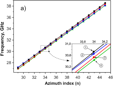
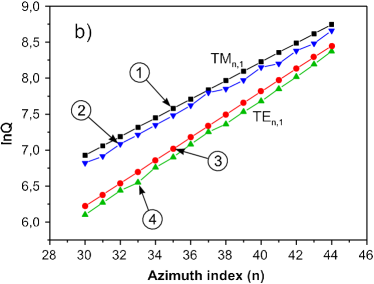
Figure 3: (Color online) The collation of theoretic and experimental data for the DDR with perfect cylindrical boundaries: the dependence a) of spectral line frequency and b) of the logarithm of quality factor on the azimuth index $n$. For $\mathrm{TM_{n,1}}$ mode: 1 —calculation, 2 — experiment; for $\mathrm{TE_{n,1}}$ mode: 3 — calculation, 4 — experiment.

dissipation loss in the dielectric, and experimentally measured frequencies is no more than 1%. The quality factors obtained in the experiment (as shown in Fig. 3b) are smaller than those calculated theoretically. We attribute this to the fact that the measured $Q$-factor includes not only eigen-loss in the resonator material but also is affected by the loss resulting from coupling with the antenna. From the diagrams in Fig. 3 one can observe the nearly equidistant character of the spectrum (the frequency interval $\Delta\nu\cong 0.7$ GHz), which is typical for open resonators with WG-type oscillations bib:Vainstein88 , as well as the exponential dependence on the mode index $n$ of the calculated and the measured $Q$-factors.

Our calculations suggested, and that was experimentally confirmed, that for TM oscillations the resonator quality factor is significantly larger than that for TE oscillations, both of them being taken with the same azimuth index. This suggests that in the case of TM oscillations the DDR has the property to more efficiently retain electromagnetic field in its volume than the resonator with TE oscillations does. We have thus established that both the theoretical model of the resonator we have chosen for our calculations and the characteristic equations obtained thereupon have found impressive experimental confirmations.

According to the findings of our theory, the main physical mechanism for EM field scattering by random inhomogeneities of the resonator side boundaries is the gradient mechanism. The scattering arisen due to fluctuations in the asperity slope can be allowed for by way of modification of the cylindrical functions indices along with the wave numbers in the characteristic equation Eq. (33). The modification reduces to multiplying the parameters $n$, $k$, $k_{\perp}$ and $k_{\perp}^{\varepsilon}$ by factor of $\chi=\left(1+\Xi^{2}\right)^{-1/2}<1$. In order to identify the main scattering mechanism experimentally and thus to check the developed theory it was necessary to estimate the value of the parameter $\Xi$ starting from the parameters relevant to a particular experiment. We were governed by the following considerations. Setting the correlation length equal to an average distance between the centers of the attached dielectric bracket-bars, i. e., $s_{c}=2\pi R/N$, where $N$ is the total number of the bracket-bars, with Gaussian distributed inhomogeneities we obtain

$$\chi=\left[1+\left(\frac{\sigma N}{R}\right)^{2}\right]^{-1/2}\ .$$ (34)

It can be easily seen that the parameter $\chi$ tends to decrease with an increasing number of bracket-bars, which leads to a decrease in the effective wave number $\widetilde{k}$ and the effective mode index $\widetilde{n}$. Since the dependence of the quality factor on the mode index is nearly exponential, $Q\approx\mathrm{e}^{\widetilde{n}}$, the availability of surface inhomogeneities should result in the decrease in the resonator quality factor, whose origin is not an additional dissipative loss.

According to our theory, with a small number of inhomogeneities the effect of slope-controlled scattering must be fairly slight (the parameter $\Xi$ decreases with lowering $N$). Therefore the value of quality factor must be weakly dependent on $N$ as well. Such was indeed the case in our experiments whose results are depicted in Fig. 4.

.4in

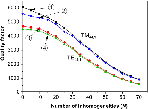
Figure 4: (Color online) The $Q$-factor curves versus the number of inhomogeneities on the resonator side surface. $\mathrm{TM}_{44,1}$ oscillations: 1 — theory, 2 — experiment; $\mathrm{TE}_{44,1}$ oscillations; 3 — theory, 4 — experiment. Calculations were carried out at $\sigma=3.5$ mm and $R=51$ mm.

In the same figure, the curves $Q(N)$ are plotted for comparison, which are calculated from characteristic equation (33) including modification factor $\chi$ and the dissipation loss in the resonator material. The loss was taken into consideration phenomenologically, by adding the imaginary part to permittivity $\varepsilon$, see Eq. (5). With the statistical nature of our measurements (the averaging is done over a large number of realizations of the bracket-bar set), the agreement between theoretical and experimental results appears to be quite satisfactory. This suggests that, since both in our theory and in the numerical calculations based upon it the slope scattering mechanism alone is taken into account, the qualitative agreement between theory and experiment unambiguously corroborates the dominant role of this particular type of wave-surface scattering.

As is also seen from Fig. 4, the influence of surface inhomogeneities on the DDR spectrum differs significantly for TE- and TM-type oscillations. The quality factors of TE oscillations are to a far larger extent subjected to the resonator boundary roughness as against the factors of TM oscillations. With a given number of inhomogeneities, the $Q$-factor of TE oscillations is noticeably smaller than that of TM oscillations. This fact, which is quite important for practical applications of microresonators in laser oscillation systems, was given certain attention in Ref. bib:Borselli2004 . Yet in the present work it has been comprehensively substantiated.

VI Conclusion

To summarize, we have investigated spectral properties of a dielectric disk resonator with randomly rough side boundary both theoretically and experimentally. It is shown that the azimuth modes of the resonator oscillations can be rigorously separated at whatever level of surface inhomogeneities. This allowed us to obtain the asymptotically exact dispersion equations which are valid over a wide range of the roughness parameters. The only requirement imposed on the inhomogeneities and effectively utilized in the calculations was that their mean-square height be small as compared with the unperturbed (i. e., non-rough) disk resonator radius.

In deriving dispersion relations, we have shown that electromagnetic wave scattering resulting from the boundary roughness can be described in terms of two fundamentally different physical mechanisms, specifically, the amplitude (the height) scattering mechanism and the gradient (the slope) mechanism. For the first of them, the ratio of the mean height of the asperities to the oscillation wavelength (the Rayleigh parameter) acts as the main guiding parameter whereas for the gradient mechanism the mean slope of the asperities relative to the unperturbed resonator boundary plays the same role. Our estimations have revealed that it is exactly the gradient scattering that is of primary importance for the formation of rough resonator spectrum. The effect of this type of scattering can be described through the approximate dispersion equation that differs from the analogous equation for the ideally circular DDR by the gradient renormalization of the basic wave parameters, i. e,, the mode wave numbers and the azimuth index.

Our theory aimed at describing the influence of random surface inhomogeneities on microresonator spectral properties analytically is actually of model nature. The point is that it does not incorporate the electromagnetic fields radiated from the resonator into external angle sectors. To neglect these fields theoretically is quite a challenge. Therefore, to verify the conclusions of our approximate (to the certain extent) theory we have made experimental measurements on the model millimeter wave band dielectric disk resonator. Surface inhomogeneities were presented by teflon bracket-bars of relatively small cross-section, which were attached randomly to the resonator side boundary. For the perfect-wall resonator, i. e. the resonator with no inhomogeneities attached, our measurement data have demonstrated excellent agreement with the developed theory concerning both the frequency spectrum and the quality factors of spectral lines. Close qualitative agreement is also attained with regard to the effect produced on the resonator spectrum by random surface inhomogeneities placed at the side boundary. First, we have confirmed the theoretical predictions about the leading role of the gradient scattering mechanism in describing the effect of random rough boundaries. Second, we ascertained that the system of model dispersion equations we have obtained herein is quite effective in describing the open microresonator spectra.

Besides, our experiments have revealed that the effect produced by the surface inhomogeneities of the DDR on the TE and TM oscillation spectra is fundamentally different. The TM oscillations quality factor exceeds significantly the analogous factor for the TE oscillations, being yet less affected by surface inhomogeneities. In our work this particular fact, which is essential for the production of microresonator-based lasers, has been theoretically and experimentally validated.

Appendix A Model spectrum of ideal cylindrical DDR

Proceeding from the methodology considerations, we outline the technique for deriving dispersion equations for cylindrical finite-size resonator with perfectly smooth bounding surfaces.

Consider equation (4) without potentials $\hat{V}^{(h)}$ and $\hat{V}^{(s)}$. Upon going to Fourier representation over angle variable $\varphi$ using the complete set of eigenfunctions $\bm{|}\varphi,n\bm{\rangle}=(2\pi)^{-1/2}\exp(-in\varphi)$, where $n=0,\pm 1,\pm 2,\ldots\$, the equation for $n$-th angular component of the wave function becomes

$$\left[\frac{1}{r}\frac{\partial}{\partial r}r\frac{\partial}{\partial r}+\frac{\partial^{2}}{\partial z^{2}}+K^{2}(r,z)-\frac{n^{2}}{r^{2}}\right]\Psi_{n}(r,z)=0\ .$$ (35)

The function $\Psi_{n}(r,z)$ is sought to be finite as $r\rightarrow 0$, whereas at $r\rightarrow\infty$ and $|z|\to\infty$ the radiation conditions are meant to be fulfilled.

It is difficult to find the explicit solution of Eq. (35) in the entire domain of variables $r$ and $z$. Yet basically there is no need to make use of such a solution. It will suffice to obtain dispersion relations which are not strictly valid but satisfied with good accuracy. We will seek a desired solution in the model form, as was done, e. g., in Refs. bib:IvanovKalin1988 ; bib:Peng96 , imposing the pair of basic requirements. One of the requirements is to fulfil fundamental boundary conditions at zero and infinite distances from the resonator center, while the other is to provide correct joining of the EM field components at the dielectric disk interfaces.

By representing the solution of Eq. (35) as a sum of $E_{z}$-symmetric and $E_{z}$-antisymmetric summands (hereinafter we will specify them by indices ($s$) and ($a$), respectively) we will seek the Debye potentials in the form given below,

$$U_{n1}^{(s)}(r,z)=A_{n}^{e(s)}J_{n}(k_{\perp}^{\varepsilon}r)\cos k_{z}z\ ,$$ (36a)

$$U_{n2}^{(s)}(r,z)=B_{n}^{e(s)}H_{n}^{(1)}(k_{\perp}r)\cos k_{z}z\ ,$$ (36b)

$$U_{n3}^{(s)}(r,z)=C_{n}^{e(s)}J_{n}(k_{\perp}^{\varepsilon}r)\exp(-\varkappa_{z}|z|)\ ,$$ (36c)

$$V_{n1}^{(s)}(r,z)=A_{n}^{m(s)}J_{n}(k_{\perp}^{\varepsilon}r)\sin k_{z}z\ ,$$ (37a)

$$V_{n2}^{(s)}(r,z)=B_{n}^{m(s)}H_{n}^{(1)}(k_{\perp}r)\sin k_{z}z\ ,$$ (37b)

$$V_{n3}^{(s)}(r,z)=C_{n}^{m(s)}J_{n}(k_{\perp}^{\varepsilon}r)\exp(-\varkappa_{z}|z|)\mathrm{\,sgn\,}z\ .$$ (37c)

In Eqs. (36) and (37), the subscripts 1, 2, 3

.8in

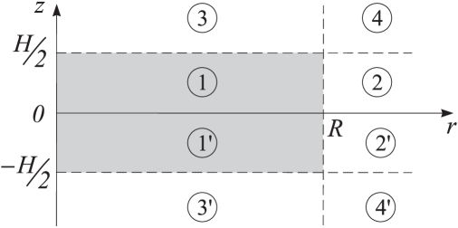
Figure 5: The areas on the half-plane $(r,z)$ between which the joining of EM fields is performed. The shaded region is filled up with the dielectric.

correspond to the regions (see Fig. 5) which are labeled with corresponding numbers. The wave parameters $k_{\perp}$, $k_{\perp}^{\varepsilon}$ and $\varkappa_{z}$ are given by

$$k_{\perp}^{2}=k^{2}-k_{z}^{2}\ ,$$ (38a)

$${(k_{\perp}^{\varepsilon})}^{2}=\varepsilon k^{2}-k_{z}^{2}\ ,$$ (38b)

$$\varkappa_{z}^{2}=k^{2}(\varepsilon-1)-k_{z}^{2}\ .$$ (38c)

By representing EM field components in terms of the potentials (36) and (37) and by joining the in- and the out- field components at the resonator side boundary (i. e., between regions 1 and 2) we obtain the well-known equation that couples together wave parameters $k$ and $k_{z}$ bib:Vainstein88 ,

$$\left[\frac{\varepsilon}{k_{\perp}^{\varepsilon}}\frac{{J_{n}}^{\prime}(k_{\perp}^{\varepsilon}R)}{J_{n}(k_{\perp}^{\varepsilon}R)}-\frac{1}{k_{\perp}}\frac{{H_{n}^{(1)}}^{\prime}(k_{\perp}R)}{H_{n}^{(1)}(k_{\perp}R)}\right]\Bigg{[}\frac{1}{k_{\perp}^{\varepsilon}}\frac{{J_{n}}^{\prime}(k_{\perp}^{\varepsilon}R)}{J_{n}(k_{\perp}^{\varepsilon}R)}-\frac{1}{k_{\perp}}\frac{{H_{n}^{(1)}}^{\prime}(k_{\perp}R)}{H_{n}^{(1)}(k_{\perp}R)}\Bigg{]}=\frac{n^{2}}{R^{2}}(\varepsilon-1)^{2}\frac{k_{z}^{2}k^{2}}{{(k_{\perp}^{\varepsilon})}^{4}k_{\perp}^{4}}\ .$$ (39)

In order to obtain yet another coupling equation for the same wave parameters we join the tangential components of the field at the end boundary ${z=H/2}$. This leads to the set of equations

$$k_{\perp}^{\varepsilon}{J_{n}}^{\prime}(k_{\perp}^{\varepsilon}r)\bigg{[}-k_{z}\sin\frac{k_{z}H}{2}A_{n}^{e(s)}+\varkappa_{z}\exp\big{(}-\varkappa_{z}H/2\big{)}C_{n}^{e(s)}\bigg{]}$$

$$\hskip 142.26378pt+\frac{n}{r}J_{n}(k_{\perp}^{\varepsilon}r)\,k\bigg{[}\sin\frac{k_{z}H}{2}A_{n}^{m(s)}-\exp\big{(}-\varkappa_{z}H/2\big{)}C_{n}^{m(s)}\bigg{]}=0\ ,$$ (40a)

$$k_{\perp}^{\varepsilon}{J_{n}}^{\prime}(k_{\perp}^{\varepsilon}r)\,k\bigg{[}\sin\frac{k_{z}H}{2}A_{n}^{m(s)}-\exp\big{(}-\varkappa_{z}H/2\big{)}C_{n}^{m(s)}\bigg{]}$$

$$\hskip 142.26378pt+\frac{n}{r}J_{n}(k_{\perp}^{\varepsilon}r)\bigg{[}-k_{z}\sin\frac{k_{z}H}{2}A_{n}^{e(s)}+\varkappa_{z}\exp\big{(}-\varkappa_{z}H/2\big{)}C_{n}^{e(s)}\bigg{]}=0\ ,$$ (40b)

$$k_{\perp}^{\varepsilon}{J_{n}}^{\prime}(k_{\perp}^{\varepsilon}r)\bigg{[}k_{z}\cos\frac{k_{z}H}{2}A_{n}^{m(s)}+\varkappa_{z}\exp\big{(}-\varkappa_{z}H/2\big{)}C_{n}^{m(s)}\bigg{]}$$

$$\hskip 142.26378pt-\frac{n}{r}J_{n}(k_{\perp}^{\varepsilon}r)\,k\bigg{[}\varepsilon\cos\frac{k_{z}H}{2}A_{n}^{e(s)}-\exp\big{(}-\varkappa_{z}H/2\big{)}C_{n}^{e(s)}\bigg{]}=0\ ,$$ (40c)

$$k_{\perp}^{\varepsilon}{J_{n}}^{\prime}(k_{\perp}^{\varepsilon}r)\,k\bigg{[}\varepsilon\cos\frac{k_{z}H}{2}A_{n}^{e(s)}-\exp\big{(}-\varkappa_{z}H/2\big{)}C_{n}^{e(s)}\bigg{]}$$

$$\hskip 142.26378pt-\frac{n}{r}J_{n}(k_{\perp}^{\varepsilon}r)\bigg{[}k_{z}\cos\frac{k_{z}H}{2}A_{n}^{m(s)}+\varkappa_{z}\exp\big{(}-\varkappa_{z}H/2\big{)}C_{n}^{m(s)}\bigg{]}=0\ ,$$ (40d)

where the number of the unknowns (to the latter we assign not only constant factors included in Eqs. (36) and (37)) but also the functions ${J_{n}}^{\prime}(k_{\perp}^{\varepsilon}r)$ and $(n/r)J_{n}(k_{\perp}^{\varepsilon}r)$) exceeds the number of the equations thus obtained. The situation can be improved if one adds to the system (40) a pair of equalities resulting from joining the EM field normal components at the same end boundary, specifically,

$$A_{n}^{e(s)}\cos\frac{k_{z}H}{2} =\frac{1}{\varepsilon}C_{n}^{e(s)}\exp\big{(}-\varkappa_{z}H/2\big{)}\ ,$$ (41a)

$$A_{n}^{m(s)}\sin\frac{k_{z}H}{2} =C_{n}^{m(s)}\exp\big{(}-\varkappa_{z}H/2\big{)}\ .$$ (41b)

Using Eqs. (40) and (41) we arrive at a set of four coupled equations which can be naturally combined in pairs, viz.

$$\left\{\begin{aligned} k_{\perp}^{\varepsilon}{J_{n}}^{\prime}(k_{\perp}^{\varepsilon}r)\left(\varkappa_{z}-\frac{k_{z}}{\varepsilon}\tan\frac{k_{z}H}{2}\right)C_{n}^{e(s)}=0\ ,\\ \frac{n}{r}J_{n}(k_{\perp}^{\varepsilon}r)\left(\varkappa_{z}-\frac{k_{z}}{\varepsilon}\tan\frac{k_{z}H}{2}\right)C_{n}^{e(s)}=0\ ,\end{aligned}\right.$$ (42a)

$$\left\{\begin{aligned} k_{\perp}^{\varepsilon}{J_{n}}^{\prime}(k_{\perp}^{\varepsilon}r)\left(\varkappa_{z}+k_{z}\cot\frac{k_{z}H}{2}\right)C_{n}^{m(s)}=0\ ,\\ \frac{n}{r}J_{n}(k_{\perp}^{\varepsilon}r)\left(\varkappa_{z}+k_{z}\cot\frac{k_{z}H}{2}\right)C_{n}^{m(s)}=0\ .\end{aligned}\right.$$ (42b)

Since the Bessel functions do not vanish simultaneously with their derivatives, one can satisfy Eqs. (42) in two ways. The first one is to equate the expression in parenthesis of Eq. (42a) to zero, putting the constant ${C_{n}^{m(s)}=0}$ in Eqs. (42b). Alternatively, the parenthesis in Eq. (42b) can be set equal to zero concurrently with the coefficient $C_{n}^{e(s)}$ in Eqs. (42a). As can be readily seen from Eqs. (36) and (37), the former solution corresponds to the TM-type oscillations whereas the latter is consistent with TE polarization. Both of these cases can be combined into one equation of the following form

$$\bigg{(}\underbrace{\varkappa_{z}-\frac{k_{z}}{\varepsilon}\tan\frac{k_{z}H}{2}}_{\mathrm{TM}}\bigg{)}\bigg{(}\underbrace{\varkappa_{z}+k_{z}\cot\frac{k_{z}H}{2}}_{\mathrm{TE}}\bigg{)}=0\ .$$ (43)

The lower curly brackets in Eq. (43) indicate the polarization which correlates with vanishing the expression in the corresponding parenthesis. By carrying out the calculations similar to those given above, for $E_{z}$-antisymmetric solution of Eq. (35) we arrive, instead of Eq. (43), at the equality

$$\bigg{(}\underbrace{\varkappa_{z}-k_{z}\tan\frac{k_{z}H}{2}}_{\mathrm{TE}}\bigg{)}\bigg{(}\underbrace{\varkappa_{z}+\frac{k_{z}}{\varepsilon}\cot\frac{k_{z}H}{2}}_{\mathrm{TM}}\bigg{)}=0\ .$$ (44)

Note that the relationships (39), (43) and (44) were previously obtained in Ref. bib:IvanovKalin1988 , although the latter two of them were of somewhat different form. In that paper, however, polarization of the excited EM field was not discussed at all. At first glance, from our derivation of Eqs. (43) and (44) it may seem that TM- and TE-type oscillations in the DDR of finite thickness can be perfectly separated, at least, with no regard for the boundary inhomogeneity. As a matter of fact, this is not the case because one must take into account the inaccuracy, i. e., the model character of wave solutions (36) and (37) used when deriving dispersion relations. These solutions, as well as the analogous ones for the antisymmetric case, are well adapted for joining the in- and the out- field components at the boundaries between regions 1–2 and 1–3 in Fig. 5. The fields in region 4 are not taken into consideration, which must inevitably result in some “overflow” of the spectrum obtained in such a way.

It is a difficult task to correctly evaluate the possibility to neglect the fields in the 4-th region in Fig. 5 without resorting to rigorous calculations. Nevertheless, by now there does not exist a rigorous theory for a finite thickness DDR, even in the seemingly simple case where the boundaries are perfectly smooth. For this reason, in order to test the results we obtained by the model calculations we choose to compare the spectrum resulting from Eqs. (33), (43), (44) with the one measured in the experiment.

Appendix B Mode separation in two-dimensional wave equation with arbitrary scattering potential

Consider the equation for Green function of Eq. (13) without rendering both the physical nature of mode potentials and their absolute value concrete,

$$\left[\frac{1}{r}\frac{\partial}{\partial r}r\frac{\partial}{\partial r}+\widetilde{K}_{\perp}^{2}(r|z_{\scriptscriptstyle\lessgtr})-\frac{\widetilde{n}^{2}}{r^{2}}-\widetilde{\mathcal{V}}_{n}(r|z_{\scriptscriptstyle\lessgtr})\right]G_{nn^{\prime}}(r,r^{\prime}|z)-\sum_{m\neq n}\widetilde{\mathcal{U}}_{nm}(r|z_{\scriptscriptstyle\lessgtr})G_{mn^{\prime}}(r,r^{\prime}|z_{\scriptscriptstyle\lessgtr})=\frac{1}{r}\delta(r-r^{\prime})\delta_{nn^{\prime}}\ .$$ (45)

Along with the exact Green function, which has a matrix structure in variables $n$ and $r$, we introduce for each of the azimuth modes the trial mode propagator, which is assumed to obey the closed equation

$$\left[\frac{1}{r}\frac{\partial}{\partial r}r\frac{\partial}{\partial r}+\widetilde{K}_{\perp}^{2}(r|z_{\scriptscriptstyle\lessgtr})-\frac{\widetilde{n}^{2}}{r^{2}}-\widetilde{\mathcal{V}}_{n}(r|z_{\scriptscriptstyle\lessgtr})\right]G^{(V)}_{n}(r,r^{\prime}|z_{\scriptscriptstyle\lessgtr})=\frac{1}{r}\delta(r-r^{\prime})$$ (46)

resulting from Eq. (45) providing that the inter-mode scattering is disregarded. We will use the notation $\hat{G}^{(V)-1}_{n}$ for the operator in square brackets of Eq. (46). The initial equation (45) can then be recast as

$$\hat{G}^{(V)-1}_{n}G_{nn^{\prime}}(r,r^{\prime}|z_{\scriptscriptstyle\lessgtr})=\frac{1}{r}\delta(r-r^{\prime})\delta_{nn^{\prime}}+\sum_{m\neq n}\widetilde{\mathcal{U}}_{nm}(r|z_{\scriptscriptstyle\lessgtr})G_{mn^{\prime}}(r,r^{\prime}|z_{\scriptscriptstyle\lessgtr})\ ,$$ (47)

or, in the equivalent integral form, as

$$G_{nn^{\prime}}(r,r^{\prime}|z_{\scriptscriptstyle\lessgtr})=G_{n}^{(V)}(r,r^{\prime}|z_{\scriptscriptstyle\lessgtr})\delta_{nn^{\prime}}+\sum_{m\neq n}\int\limits_{0}^{\infty}r_{1}dr_{1}G_{n}^{(V)}(r,r_{1}|z_{\scriptscriptstyle\lessgtr})\widetilde{\mathcal{U}}_{nm}(r_{1}|z_{\scriptscriptstyle\lessgtr})G_{mn^{\prime}}(r_{1},r^{\prime}|z_{\scriptscriptstyle\lessgtr})\ .$$ (48)

By setting in Eq. (48) index $n\neq n^{\prime}$ and then re-labelling all mode indices we can write this equation as the equation for solely inter-mode components of the Green matrix $\|G_{mn}\|$, the intra-mode ones being thought of as known functions,

$$G_{mn}(r,r^{\prime}|z_{\scriptscriptstyle\lessgtr})-\sum_{\genfrac{}{}{0.0pt}{}{k\neq m}{k\neq n}}\int\limits_{0}^{\infty}r_{1}dr_{1}G_{m}^{(V)}(r,r_{1}|z_{\scriptscriptstyle\lessgtr})\widetilde{\mathcal{U}}_{mk}(r_{1}|z_{\scriptscriptstyle\lessgtr})G_{kn}(r_{1},r^{\prime}|z_{\scriptscriptstyle\lessgtr})=\int\limits_{0}^{\infty}r_{1}dr_{1}G_{m}^{(V)}(r,r_{1}|z_{\scriptscriptstyle\lessgtr})\widetilde{\mathcal{U}}_{mn}(r_{1}|z)G_{nn}(r_{1},r^{\prime}|z_{\scriptscriptstyle\lessgtr})\ .$$ (49)

At this stage we introduce three operators, $\hat{\mathcal{G}}^{(V)}$, $\hat{\mathcal{U}}$ and $\hat{\mathsf{R}}$, which are assumed to act in the reduced coordinate-mode space $\mathsf{\overline{M}}_{n}$ consisting of the half-axis $r\geqslant 0$ and the entire set of mode indices except for particular index $n$. The operators are specified by their matrix elements

$$\bm{\langle}r,n\bm{|}\hat{\mathcal{G}}^{(V)}\bm{|}r^{\prime},m\bm{\rangle}=G^{(V)}_{n}(r,r^{\prime}|z_{\scriptscriptstyle\lessgtr})\delta_{nm}\ ,$$ (50a)

$$\bm{\langle}r,n\bm{|}\hat{\mathcal{U}}\bm{|}r^{\prime},m\bm{\rangle}=\widetilde{\mathcal{U}}_{nm}(r|z_{\scriptscriptstyle\lessgtr})\frac{1}{r}\delta(r-r^{\prime})\ ,$$ (50b)

$$\bm{\langle}r,n\bm{|}\hat{\mathsf{R}}\bm{|}r^{\prime},m\bm{\rangle}=G^{(V)}_{n}(r,r^{\prime}|z)\widetilde{\mathcal{U}}_{nm}(r^{\prime}|z_{\scriptscriptstyle\lessgtr})\ .$$ (50c)

Equation (49) can now be recast as the matrix equality

$$\bm{\langle}r,m\bm{|}\big{(}1-\hat{\mathsf{R}}\big{)}\hat{\mathcal{G}}\bm{|}r^{\prime},n\bm{\rangle}=\bm{\langle}r,m\bm{|}\hat{\mathsf{R}}\bm{P}_{n}\hat{\mathcal{G}}\bm{|}r^{\prime},n\bm{\rangle}\ ,$$ (51)

or, equivalently, in the general operator form as $\bm{P}_{m}\big{(}1-\hat{\mathsf{R}}\big{)}\hat{\mathcal{G}}\bm{P}_{n}=\bm{P}_{m}\hat{\mathsf{R}}\bm{P}_{n}\hat{\mathcal{G}}\bm{P}_{n}$. Here, $\bm{P}_{n}$ is the projection operator whose action reduces to assigning the value $n$ to the nearest mode index of an arbitrary operator standing adjacent to it, either to the left or right. Multiplying both sides of the operator equality thus obtained by the operator $\big{(}1-\hat{\mathsf{R}}\big{)}^{-1}$ whose regularity was substantiated in Ref. bib:Tar00 we arrive at the integral relation between the non-diagonal and diagonal mode matrix elements of the Green function, viz.

$$G_{mn}(r,r^{\prime}|z_{\scriptscriptstyle\lessgtr})=\bm{\langle}r,m\bm{|}\big{(}1-\hat{\mathsf{R}}\big{)}^{-1}\hat{\mathsf{R}}\bm{P}_{n}\hat{\mathcal{G}}\bm{|}r^{\prime},n\bm{\rangle}=\big{(}\hat{K}_{mn}\hat{G}_{nn}\big{)}(r,r^{\prime}|z_{\scriptscriptstyle\lessgtr})\ .$$ (52)

Setting in Eq. (45) index $n^{\prime}=n$ and substituting the inter-mode propagators in the form (52) we eventually obtain the closed equation for intra-mode Green function $G_{nn}(r,r^{\prime}|z_{\scriptscriptstyle\lessgtr})$,

$$\left[\frac{1}{r}\frac{\partial}{\partial r}r\frac{\partial}{\partial r}+\widetilde{K}_{\perp}^{2}(r|z_{\scriptscriptstyle\lessgtr})-\frac{\widetilde{n}^{2}}{r^{2}}-\widetilde{\mathcal{V}}_{n}(r|z_{\scriptscriptstyle\lessgtr})-\hat{\mathcal{T}}_{n}\right]G_{nn}(r,r^{\prime}|z_{\scriptscriptstyle\lessgtr})=\frac{1}{r}\delta(r-r^{\prime})\ .$$ (53)

Here, $\hat{\mathcal{T}}_{n}$ is the operator that accounts for the inter-mode scattering (it is just the $T$-matrix well-known in quantum scattering theory bib:Newton68 ; bib:Taylor72 ), which has the form

$$\hat{\mathcal{T}}_{n}=\bm{P}_{n}\hat{\mathcal{U}}\big{(}\openone-\hat{\mathsf{R}}\big{)}^{-1}\hat{\mathsf{R}}\bm{P}_{n}\ .$$ (54)

Trial Green function $G^{(V)}_{n}(r,r^{\prime}|z_{\scriptscriptstyle\lessgtr})$ entering operator potential (54) through matrix elements (50c) obeys equation (46) and the same boundary conditions just like the desired mode propagator $G_{nn}(r,r^{\prime}|z_{\scriptscriptstyle\lessgtr})$.

Equation (53) along with Eq. (52) determines the entire Green function of wave equation (13) and serves as a basis for deriving the system of uncoupled equations (15) for azimuth components of the sought-for wave function.

References

- (1) A. Polman, B. Min, J. Kalkman, T. J. Kippenberg, and K. J. Vahala, Appl. Phys. Lett. 84, 1037 (2004).
- (2) K. J. Vahala, Nature 424, 839 (2003).
- (3) E. M. Ganapolskii, Z. E. Eremenko, and Yu. V. Tarasov, Phys. Rev. E75, 026212 (2007).
- (4) B. E. Little, J.-P. Laine, and S. T. Chu, Opt. Lett. 22, 4 (1997).
- (5) M. L. Gorodetsky and A. D. Pryamikov, J. Opt. Soc. Am. B 17, 1051 (2000).
- (6) A. N. Oraevsky, Quantum Electron.32(5), 377 (2002).
- (7) M. Borselli, K. Srinivasan, P. E. Barclay, and O. Painter, Appl. Phys. Lett. 85, 3693 (2004).
- (8) M. Kuznetsov and H. A. Haus, IEEE J. Quan. Elec. 19, 1505 (1983).
- (9) F. G. Bass and I. M. Fuks, Wave Scattering from Statistically Rough Surfaces (New York: Pergamon, 1979)
- (10) J. A. Ogilvy, Theory of Wave Scattering from Random Rough Surfaces (IOP Pub., Bristol, UK, 1991).
- (11) A.G. Voronovich, Wave Scattering from Rough Surfaces (Springer Verlag, 1994).
- (12) Lord Rayleigh, Proc. R. Soc. London Ser. A 79, 399 (1907).
- (13) Lord Rayleigh, The Theory of Sound, (Dover, New-York, 1945).
- (14) N. M. Makarov and Yu. V. Tarasov, J. Phys.: Condens. Matter 10, 1523 (1998).
- (15) N. M. Makarov and Yu. V. Tarasov, Phys. Rev. B64, 235306 (2001).
- (16) L. A. Vainshtein, Electromagnetic Waves [in Russian] (Radio i Svyaz, Moscow, 1988).
- (17) E. Ivanov and V. I. Kalinichev, Radiotechnika [in Russian], No. 10, 86 (1988).
- (18) H. Peng, IEEE Trans. Microwave Theory Tech. 44, 848 (1996).
- (19) G. Annillo, M. Cassettari, I. Longo, and M. Martinelli, Chem. Phys. Lett. 281, 306 (1997).
- (20) Yu. V. Tarasov, Waves Random Media 10, 395 (2000).
- (21) Yu. V. Tarasov, Low. Temp. Phys. 29, 45 (2003).
- (22) Yu. V. Tarasov, Phys. Rev. B71, 125112 (2005).
- (23) A. N. Kolmogorov, S. V. Fomin . Elements of the Theory of Functions and Functional Analysis (Dover, New York, 1961).
- (24) T. Kato. Perturbation Theory for Linear Operators (Springer, Berlin, 1966).
- (25) R. Newton. Scattering Theory of Waves and Particles (McGraw-Hill, New York, 1968).
- (26) J. R. Taylor. Scattering Theory. The Quantum Theory on Nonrelativistic Collisions (Wiley, New York, 1972).