The length of unknotting tunnels

Abstract.

We show there exist tunnel number one hyperbolic 3–manifolds with arbitrarily long unknotting tunnel. This provides a negative answer to an old question of Colin Adams.

1. Introduction

In a paper published in 1995 [1], Colin Adams studied geometric properties of hyperbolic tunnel number one manifolds. A tunnel number one manifold is defined to be a compact orientable 3–manifold $M$ with torus boundary component(s), which contains a properly embedded arc $\tau$, the exterior of which is a handlebody. The arc $\tau$ is defined to be an unknotting tunnel of $M$.

When a tunnel number one manifold $M$ admits a hyperbolic structure, there is a unique geodesic arc in the homotopy class of $\tau$. If $\tau$ runs between distinct boundary components, Adams showed that its geodesic representative has bounded length, when measured in the complement of a maximal horoball neighborhood of the cusps. He asked a question about the more general picture: does an unknotting tunnel in a hyperbolic 3–manifold always have bounded length?

In response, Adams and Reid showed that when the tunnel number one manifold is a 2–bridge knot complement, that unknotting tunnels have bounded length [2]. Akiyoshi, Nakagawa, and Sakuma showed that unknotting tunnels in punctured torus bundles actually have length zero [3], hence bounded length.

Sakuma and Weeks also studied unknotting tunnels in 2–bridge knots [18]. They found that any unknotting tunnel of a 2–bridge knot was isotopic to an edge of the canonical polyhedral decomposition of that knot, first explored by Epstein and Penner [8]. They conjectured that all unknotting tunnels were isotopic to edges of the canonical decomposition. Heath and Song later showed by example that not all unknotting tunnels could be isotopic to edges of the canonical decomposition [10]. However, the question of whether unknotting tunnels have bounded length remained unanswered.

In this paper we finally settle the answer to this question. We show that, in fact, the answer is no. There exist tunnel number one manifolds with arbitrarily long unknotting tunnel.

Theorem 4.1.

There exist finite volume one–cusped hyperbolic tunnel number one manifolds for which the geodesic representative of the unknotting tunnel is arbitrarily long, as measured between the maximal horoball neighborhood of the cusp.

Note we are not claiming here that the unknotting tunnel in these examples is ambient isotopic to a geodesic. Such examples can in fact be constructed, but the argument is more complex and will appear in a companion paper [11]. However, note that Theorem 4.1 does force the unknotting tunnels in these examples to be arbitrarily long, because the length of a properly embedded arc is at least that of the geodesic in its homotopy class.

We prove Theorem 4.1 in two ways. The first proof, which appears in Section 4, is geometric and partially non-constructive. We analyze the infinite–volume hyperbolic structures on the compression body $C$ with negative boundary a torus, and positive boundary a genus 2 surface. A guiding principle is that geometric properties of hyperbolic structures on $C$ should often have their counterparts in finite–volume hyperbolic 3–manifolds with tunnel number one. For example, any geometrically infinite hyperbolic structure on $C$ is the geometric and algebraic limit of a sequence of geometrically finite hyperbolic structures on $C$, and it is also the geometric limit of a sequence of finite–volume hyperbolic 3–manifolds with tunnel number one. It is by finding suitable sequences of hyperbolic structures on $C$ that Theorem 4.1 is proved. In particular, the proof gives very little indication of what the finite–volume hyperbolic 3–manifolds actually are.

The geometric proof of Theorem 4.1 leads naturally to the study of geometrically finite structures on the compression body $C$ and their geometric properties. We include some background material in Sections 2 and 3. However, we postpone a more extensive investigation of geometrically finite structures on $C$ to a companion paper [11].

The second proof is more topological, and appears in Section 6. The idea is to start with a tunnel number one manifold with two cusps. An argument using homology implies that there exist Dehn fillings on one cusp which yield a tunnel number one manifold whose core tunnel must be arbitrarily long.

A consequence of the second proof is that the resulting tunnel number one manifold cannot be the exterior of a knot in a homology sphere. In Section 5, we modify the construction of the first proof to show there do exist tunnel number one manifolds with long tunnel which are the exterior of a knot in a homology sphere. It seems likely that the Dehn filling construction in Section 6 can be modified to produce hyperbolic knots in homology spheres with long unknotting tunnels. However, to establish this, a substantially different method of proof would be required.

Although we construct examples of knots in homology 3–spheres with long unknotting tunnels, we do not obtain knots in the 3–sphere using our methods. It would be interesting to determine whether such sequences of knots exist. If they do, can explicit diagrams of such knots be found?

1.1. Acknowledgements

Lackenby and Purcell were supported by the Leverhulme trust. Lackenby was supported by an EPSRC Advanced Research Fellowship. Purcell was supported by NSF grant DMS-0704359. Cooper was partially supported by NSF grant DMS-0706887.

2. Background and preliminary material

In this section we will review terminology and results used throughout the paper.

The first step in the proof of Theorem 4.1 is to show there exist geometrically finite structures on a compression body $C$ with arbitrarily long tunnel. We begin by defining these terms.

2.1. Compression bodies

A compression body $C$ is either a handlebody, or the result of taking a closed, orientable (possibly disconnected) surface $S$ cross an interval $[0,1]$, and attaching 1–handles to $S\times\{1\}$. The negative boundary, denoted $\partial_{-}C$, is $S\times\{0\}$. When $C$ is a handlebody, $\partial_{-}C=\emptyset$. The positive boundary is $\partial C\setminus\partial_{-}C$, and is denoted $\partial_{+}C$.

Throughout this paper, we will be interested in compression bodies $C$ for which $\partial_{-}C$ is a torus and $\partial_{+}C$ is a genus $2$ surface. We will refer to such a manifold as a $(1,2)$–compression body, where the numbers $(1,2)$ refer to the genus of the boundary components.

Let $\tau$ be the union of the core of the attached 1–handle with two vertical arcs in $S\times[0,1]$ attached to its endpoints. Thus, $\tau$ is a properly embedded arc in $C$, and $C$ is a regular neighborhood of $\partial_{-}C\cup\tau$. We refer to $\tau$ as the core tunnel. See Figure 1.

Figure 1. The $(1,2)$–compression body. The core tunnel is the thick line shown, with endpoints on the torus boundary.

Note that the fundamental group of a $(1,2)$–compression body $C$ is isomorphic to $({\mathbb{Z}}\times{\mathbb{Z}})\ast{\mathbb{Z}}$. We will denote the generators of the ${\mathbb{Z}}\times{\mathbb{Z}}$ factor by $\alpha$, $\beta$, and we will denote the generator of the second factor by $\gamma$.

2.2. Hyperbolic structures

Let $C$ be a $(1,2)$–compression body. We are interested in complete hyperbolic structures on the interior of $C$. We obtain a hyperbolic structure on $C\setminus{\partial}C$ by taking a discrete, faithful representation $\rho\colon\thinspace\pi_{1}(C)\to{\rm PSL}(2,{\mathbb{C}})$ and considering the manifold ${\mathbb{H}}^{3}/\rho(\pi_{1}(C))$.

Definition 2.1.

A discrete subgroup $\Gamma<{\rm PSL}(2,{\mathbb{C}})$ is geometrically finite if ${\mathbb{H}}^{3}/\Gamma$ admits a finite–sided, convex fundamental domain. In this case, we will also say that the manifold ${\mathbb{H}}^{3}/\Gamma$ is geometrically finite.

Geometrically finite groups are well understood. In this paper, we will often use the following theorem of Bowditch (and its corollary, Corollary 2.10 below).

Theorem 2.2 (Bowditch, Proposition 5.7 [5]).

If a subgroup $\Gamma<{\rm PSL}(2,{\mathbb{C}})$ is geometrically finite, then every convex fundamental domain for ${\mathbb{H}}^{3}/\Gamma$ has finitely many faces.

Definition 2.3.

For $C$ a $(1,2)$–compression body, we will say that a discrete, faithful representation $\rho$ is minimally parabolic if for all $g\in\pi_{1}(C)$, $\rho(g)$ is parabolic if and only if $g$ is conjugate to an element of the fundamental group of the torus boundary component ${\partial}_{-}C$.

Definition 2.4.

A discrete, faithful representation $\rho\colon\thinspace\pi_{1}(C)\to{\rm PSL}(2,{\mathbb{C}})$ is a minimally parabolic geometrically finite uniformization of $C$ if $\rho$ is minimally parabolic, $\rho(\pi_{1}(C))$ is geometrically finite as a subgroup of ${\rm PSL}(2,{\mathbb{C}})$, and ${\mathbb{H}}^{3}/\rho(\pi_{1}(C))$ is homeomorphic to the interior of $C$.

It is a classical result, due to Bers, Kra, and Maskit (see [4]), that the space of conjugacy classes of minimally parabolic geometrically finite uniformizations of $C$ may be identified with the Teichmüller space of the genus 2 boundary component ${\partial}_{+}C$, quotiented out by ${\rm Mod}_{0}(C)$, the group of isotopy classes of homeomorphisms of $C$ which are homotopic to the identity.

In particular, note that the space of minimally parabolic geometrically finite uniformizations is path connected.

2.3. Isometric spheres and Ford domains

The tool we use to study geometrically finite representations is that of Ford domains. We define the necessary terminology in this section.

Throughout this subsection, let $M={\mathbb{H}}^{3}/\Gamma$ be a hyperbolic manifold with a single rank two cusp, for example, the $(1,2)$–compression body. In the upper half space model for ${\mathbb{H}}^{3}$, assume the point at infinity in ${\mathbb{H}}^{3}$ projects to the cusp. Let $H$ be any horosphere about infinity. Let $\Gamma_{\infty}<\Gamma$ denote the subgroup that fixes $H$. By assumption, $\Gamma_{\infty}={\mathbb{Z}}\times{\mathbb{Z}}$.

Definition 2.5.

For any $g\in\Gamma\setminus\Gamma_{\infty}$, $g^{-1}(H)$ will be a horosphere centered at a point of ${\mathbb{C}}$, where we view the boundary at infinity of ${\mathbb{H}}^{3}$ to be ${\mathbb{C}}\cup\{\infty\}$. Define the set $S_{g}$ to be the set of points in ${\mathbb{H}}^{3}$ equidistant from $H$ and $g^{-1}(H)$. $S_{g}$ is the isometric sphere of $g$.

Note that $S_{g}$ is well–defined even if $H$ and $g^{-1}(H)$ overlap. It will be a Euclidean hemisphere orthogonal to the boundary ${\mathbb{C}}$ of ${\mathbb{H}}^{3}$.

At first glance, it may seem more natural to consider points equidistant from $H$ and $g(H)$, rather than $g^{-1}(H)$ as in Definition 2.5. However, we use the historical definition of isometric spheres in order to make use of the following classical result, which we include as a lemma. A proof can be found, for example, in Maskit’s book [15, Chapter IV, Section G].

Lemma 2.6.

For any $g\in\Gamma\setminus\Gamma_{\infty}$, the action of $g$ on ${\mathbb{H}}^{3}$ is given by inversion in $S_{g}$ followed by a Euclidean isometry. ∎

The following is well known, and follows from standard calculations in hyperbolic geometry. We give a proof in [11].

Lemma 2.7.

If

$$g=\left(\begin{array}[]{cccc}a&b\\ c&d\\ \end{array}\right)\in{\rm PSL}(2,{\mathbb{C}}),$$

then the center of the Euclidean hemisphere $S_{g^{-1}}$ is $g(\infty)=a/c$. Its Euclidean radius is $1/|c|$.

Let $B_{g}$ denote the open half ball bounded by $S_{g}$. Define ${\mathcal{F}}$ to be the set

$${\mathcal{F}}={\mathbb{H}}^{3}\setminus\bigcup_{g\in\Gamma\setminus\Gamma_{\infty}}B_{g}.$$

Note ${\mathcal{F}}$ is invariant under $\Gamma_{\infty}$, which acts by Euclidean translations on ${\mathbb{H}}^{3}$.

When $H$ bounds a horoball $H_{\infty}$ that projects to an embedded horoball neighborhood about the rank 2 cusp of $M$, ${\mathcal{F}}$ is the set of points in ${\mathbb{H}}^{3}$ which are at least as close to $H_{\infty}$ as to any of its translates under $\Gamma\setminus\Gamma_{\infty}$. Such an embedded horoball neighborhood of the cusp always exists, by the Margulis lemma.

Definition 2.8.

A vertical fundamental domain for $\Gamma_{\infty}$ is a fundamental domain for the action of $\Gamma_{\infty}$ cut out by finitely many vertical geodesic planes in ${\mathbb{H}}^{3}$.

Definition 2.9.

A Ford domain of $M$ is the intersection of ${\mathcal{F}}$ with a vertical fundamental domain for the action of $\Gamma_{\infty}$.

A Ford domain is not canonical because the choice of fundamental domain for $\Gamma_{\infty}$ is not canonical. However, for the purposes of this paper, the region ${\mathcal{F}}$ in ${\mathbb{H}}^{3}$ is often more useful than the actual Ford domain.

Note that Ford domains are convex fundamental domains. Thus we have the following corollary of Bowditch’s Theorem 2.2.

Corollary 2.10.

$M={\mathbb{H}}^{3}/\Gamma$ is geometrically finite if and only if a Ford domain for $M$ has a finite number of faces.

2.4. Visible faces and Ford domains

Definition 2.11.

Let $g\in\Gamma\setminus\Gamma_{\infty}$. The isometric sphere $S_{g}$ is called visible from infinity, or simply visible, if it is not contained in $\bigcup_{h\in\Gamma\setminus(\Gamma_{\infty}\cup\Gamma_{\infty}g)}\bar{B_{h}}$. Otherwise, $S_{g}$ is called invisible.

Similarly, suppose $g,h\in\Gamma\setminus\Gamma_{\infty}$, and $S_{g}\cap S_{h}\cap{\mathbb{H}}^{3}$ is nonempty. Then the edge of intersection $S_{g}\cap S_{h}$ is called visible if $S_{g}$ and $S_{h}$ are visible and their intersection is not contained in $\bigcup_{k\in\Gamma\setminus(\Gamma_{\infty}\cup\Gamma_{\infty}g\cup\Gamma_{\infty}h)}\bar{B_{k}}$. Otherwise, it is invisible.

The faces of ${\mathcal{F}}$ are exactly those that are visible from infinity.

In the case where $H$ bounds a horoball that projects to an embedded horoball neighborhood of the rank 2 cusp of $M$, there is an alternative interpretation of visibility. An isometric sphere $S_{g}$ is visible if and only if there exists a point $x$ in $S_{g}$ such that for all $h\in\Gamma\setminus(\Gamma_{\infty}\cup\Gamma_{\infty}g)$, the hyperbolic distance $d(x,h^{-1}(H))$ is greater than the hyperbolic distance $d(x,H)$. Similarly, an edge $S_{g}\cap S_{h}$ is visible if and only if there exists a point $x$ in $S_{g}\cap S_{h}$ such that for all $k\in\Gamma\setminus(\Gamma_{\infty}\cup\Gamma_{\infty}g\cup\Gamma_{\infty}h)$, the hyperbolic distance $d(x,H)$ is strictly less than the hyperbolic distance $d(x,k^{-1}(H))$.

We present a result that allows us to identify minimally parabolic geometrically finite uniformizations.

Lemma 2.12.

Suppose $\rho\colon\thinspace\pi_{1}(C)\to{\rm PSL}(2,{\mathbb{C}})$ is a geometrically finite uniformization. Suppose none of the visible isometric spheres of the Ford domain of ${\mathbb{H}}^{3}/\rho(\pi_{1}(C))$ are visibly tangent on their boundaries. Then $\rho$ is minimally parabolic.

By visibly tangent, we mean the following. Set $\Gamma=\rho(\pi_{1}(C))$, and assume a neighborhood of infinity in ${\mathbb{H}}^{3}$ projects to the rank two cusp of ${\mathbb{H}}^{3}/\Gamma$, with $\Gamma_{\infty}<\Gamma$ fixing infinity in ${\mathbb{H}}^{3}$. For any $g\in\Gamma\setminus\Gamma_{\infty}$, the isometric sphere $S_{g}$ has boundary that is a circle on the boundary ${\mathbb{C}}$ at infinity of ${\mathbb{H}}^{3}$. This circle bounds an open disk $D_{g}$ in ${\mathbb{C}}$. Two isometric spheres $S_{g}$ and $S_{h}$ are visibly tangent if their corresponding disks $D_{g}$ and $D_{h}$ are tangent on ${\mathbb{C}}$, and for any other $k\in\Gamma\setminus\Gamma_{\infty}$, the point of tangency is not contained in the open disk $D_{k}$.

Proof.

Suppose $\rho$ is not minimally parabolic. Then it must have a rank 1 cusp. Apply an isometry to ${\mathbb{H}}^{3}$ so that the point at infinity projects to this rank 1 cusp. The Ford domain becomes a finite sided region $P$ meeting this cusp. Take a horosphere about infinity. Because the Ford domain is finite sided, we may take this horosphere about infinity sufficiently small that the intersection of the horosphere with $P$ gives a subset of Euclidean space with sides identified by elements of $\rho(\pi_{1}(C))$, conjugated appropriately.

The side identifications of this subset of Euclidean space, given by the side identifications of $P$, generate the fundamental group of the cusp. But this is a rank 1 cusp, hence its fundamental group is ${\mathbb{Z}}$. Therefore, the side identification is given by a single Euclidean translation. The Ford domain $P$ intersects this horosphere in an infinite strip, and the side identification glues the strip into an annulus. Note this implies two faces of $P$ are tangent at infinity.

Now conjugate back to our usual view of ${\mathbb{H}}^{3}$, with the point at infinity projecting to the rank 2 cusp of the $(1,2)$–compression body ${\mathbb{H}}^{3}/\rho(\pi_{1}(C))$. The two faces of $P$ tangent at infinity are taken to two isometric spheres of the Ford domain, tangent at a visible point on the boundary at infinity. ∎

Remark.

The converse to Lemma 2.12 is not true. There exist examples of geometrically finite representations for which two visible isometric spheres are visibly tangent, and yet the representation is still minimally parabolic. We see examples of this in [11].

We next prove a result which will help us identify representations which are not discrete.

Lemma 2.13.

Let $\Gamma$ be a discrete, torsion free subgroup of ${\rm PSL}(2,{\mathbb{C}})$ such that $M={\mathbb{H}}^{3}/\Gamma$ has a rank two cusp. Suppose that the point at infinity projects to the cusp, and let $\Gamma_{\infty}$ be its stabilizer in $\Gamma$. Then for all $\zeta\in\Gamma\setminus\Gamma_{\infty}$, the isometric sphere of $\zeta$ has radius at most the minimal (Euclidean) translation length of all elements in $\Gamma_{\infty}$.

Proof.

By the Margulis lemma, there exists an embedded horoball neighborhood of the rank 2 cusp of ${\mathbb{H}}^{3}/\Gamma$. Let $H_{\infty}$ be a horoball about infinity in ${\mathbb{H}}^{3}$ that projects to this embedded horoball. Let $\tau$ be the minimum (Euclidean) translation length of all nontrivial elements in the group $\Gamma_{\infty}$, say $\tau$ is the distance translated by the element $w_{\tau}$. Suppose $S_{\zeta}$ has radius $R$ strictly larger than $\tau$. Without loss of generality, we may assume $S_{\zeta}$ is visible, for otherwise there is some visible face $S_{\xi}$ which covers the highest point of $S_{\zeta}$, hence must have even larger radius.

Because the radius $R$ of $S_{\zeta}$ is larger than $\tau$, $S_{\zeta}$ must intersect $w_{\tau}(S_{\zeta})=S_{\zeta w_{\tau}^{-1}}$, and in fact, the center $w_{\tau}\zeta^{-1}(\infty)$ of $S_{\zeta w_{\tau}^{-1}}$ must lie within the boundary circle $S_{\zeta}\cap{\mathbb{C}}$.

Consider the set of points $P$ equidistant from $\zeta^{-1}(H_{\infty})$ and $w_{\tau}\zeta^{-1}(H_{\infty})$. Because these horoballs are the same size, $P$ must be a vertical plane in ${\mathbb{H}}^{3}$ which lies over the perpendicular bisector of the line segment running from $\zeta^{-1}(\infty)$ to $w_{\tau}\zeta^{-1}(\infty)$ on ${\mathbb{C}}$.

Now apply $\zeta$. This will take the plane $P$ to $S_{0}:=S_{\zeta w_{\tau}^{-1}\zeta^{-1}}$. We wish to determine the (Euclidean) radius of $S_{0}$. By Lemma 2.6, applying $\zeta$ is the same as applying an inversion in $S_{\zeta}$, followed by a Euclidean isometry. Only the inversion will affect the radius of $S_{0}$. Additionally, the radius is independent of the location of the center of the isometric sphere $S_{\zeta}$, so we may assume without loss of generality that the center of $S_{\zeta}$ is at $0\in{\mathbb{C}}$ and that the center of $S_{\zeta w_{\tau}^{-1}}$ is at $\tau\in{\mathbb{C}}$. Now inversion in a circle of radius $R$ centered at zero takes the point $\tau$ to $R^{2}/\tau$, and the point at infinity to $0$. Thus the center of $S_{0}$, which is the image of $\tau$ under $\zeta$, will be of distance $R^{2}/\tau$ from a point on the boundary of $S_{0}$, i.e. the image of $\infty$ on $P$ under $\zeta$. Hence the radius of $S_{0}$ is $R^{2}/\tau>R$. Denote $R^{2}/\tau$ by $R_{0}$. We have $R_{0}>R>\tau$.

Now we have a new face $S_{0}$ with radius $R_{0}>R>\tau$. Again we may assume it is visible. The same argument as above implies there is another sphere $S_{1}$ with radius $R_{1}>R_{0}>\tau$. Continuing, we obtain an infinite collection of visible faces of increasing radii. These must all be distinct. But this is impossible: an infinite number of distinct faces of radius greater than $\tau$ cannot fit inside a fundamental domain for $\Gamma_{\infty}$. Thus $\Gamma$ is indiscrete. ∎

The following lemma gives us a tool to identify the Ford domain of a geometrically finite manifold.

Lemma 2.14.

Let $\Gamma$ be a subgroup of ${\rm PSL}(2,{\mathbb{C}})$ with rank 2 subgroup $\Gamma_{\infty}$ fixing the point at infinity. Suppose the isometric spheres corresponding to a finite set of elements of $\Gamma$, as well as a vertical fundamental domain for $\Gamma_{\infty}$, cut out a fundamental domain $P$ for $\Gamma$. Then $\Gamma$ is discrete and geometrically finite, and $P$ must be a Ford domain of ${\mathbb{H}}^{3}/\Gamma$.

Proof.

The discreteness of $\Gamma$ follows from Poincaré’s polyhedron theorem. The fact that it is geometrically finite follows directly from the definition.

Suppose $P$ is not a Ford domain. Since the Ford domain is only well–defined up to choice of fundamental region for $\Gamma_{\infty}$, there is a Ford domain $F$ with the same choice of vertical fundamental domain for $\Gamma_{\infty}$ as for $P$. Since $P$ is not a Ford domain, $F$ and $P$ do not coincide. Because both are cut out by isometric spheres corresponding to elements of $\Gamma$, there must be additional visible faces that cut out the domain $F$ than just those that cut out the domain $P$. Hence $F$ is a strict subset of $P$, and there is some point $x$ in ${\mathbb{H}}^{3}$ which lies in the interior of $P$, but does not lie in the Ford domain.

But now consider the covering map $\phi\colon\thinspace{\mathbb{H}}^{3}\to{\mathbb{H}}^{3}/\Gamma$. This map $\phi$ glues both $P$ and $F$ into the manifold ${\mathbb{H}}^{3}/\Gamma$, since they are both fundamental domains for $\Gamma$. So consider $\phi$ applied to $x$. Because $x$ lies in the interior of $P$, and $P$ is a fundamental domain, there is no other point of $P$ mapped to $\phi(x)$. On the other hand, $x$ does not lie in the Ford domain $F$. Thus there is some preimage $y$ of $\phi(x)$ under $\phi$ which does lie in $F$. But $F$ is a subset of $P$. Hence we have $y\neq x$ in $P$ such that $\phi(x)=\phi(y)$. This is a contradiction. ∎

2.5. The Ford spine

When we glue the Ford domain into the manifold $M={\mathbb{H}}^{3}/\Gamma$, as in the proof of Lemma 2.14, the faces of the Ford domain will be glued together in pairs to form $M$.

Definition 2.15.

The Ford spine of $M$ is defined to be the image of the visible faces of ${\mathcal{F}}$ under the covering ${\mathbb{H}}^{3}\to M$.

Remark.

A spine usually refers to a subset of the manifold onto which there is a retraction of the manifold. Using that definition, the Ford spine is not strictly a spine. However, the Ford spine union the genus 2 boundary ${\partial}_{+}C$ will be a spine for the compression body.

Let $\rho$ be a geometrically finite uniformization. Recall that the domain of discontinuity $\Omega_{\rho(\pi_{1}(C))}$ is the complement of the limit set of $\rho(\pi_{1}(C))$ in the boundary at infinity ${\partial}_{\infty}{\mathbb{H}}^{3}$. See, for example, Marden [14, section 2.4].

Lemma 2.16.

Let $\rho$ be a minimally parabolic geometrically finite uniformization of a $(1,2)$–compression body $C$. Then the manifold $({\mathbb{H}}^{3}\cup\Omega_{\rho(\pi_{1}(C))})/\rho(\pi_{1}(C))$ retracts onto the boundary at infinity $(\bar{{\mathcal{F}}}\cap{\mathbb{C}})/\Gamma_{\infty}$, union the Ford spine.

Proof.

Let $H$ be a horosphere about infinity in ${\mathbb{H}}^{3}$ that bounds a horoball which projects to an embedded horoball neighborhood of the cusp of ${\mathbb{H}}^{3}/\rho(\pi_{1}(C))$. Let $x$ be any point in ${\mathcal{F}}\cap{\mathbb{H}}^{3}$. The nearest point on $H$ to $x$ lies on a vertical line running from $x$ to infinity. These vertical lines give a foliation of ${\mathcal{F}}$. All such lines have one endpoint on infinity, and the other endpoint on $\bar{{\mathcal{F}}}\cap{\mathbb{C}}$ or an isometric sphere of ${\mathcal{F}}$. We obtain our retraction by mapping the point $x$ to the endpoint of its associated vertical line, then quotienting out by the action of $\rho(\pi_{1}(C))$. ∎

To any face $F_{0}$ of the Ford spine, we obtain an associated collection of visible elements of $\Gamma$: those whose isometric sphere projects to $F_{0}$ (or more carefully, a subset of their isometric sphere projects to the face $F_{0}$). We will often say that an element $g$ of $\Gamma$ corresponds to a face $F_{0}$ of the Ford spine of $M$, meaning $S_{g}$ is visible, and (the visible subset of) $S_{g}$ projects to $F_{0}$. Note that if $g$ corresponds to $F_{0}$, then so does $g^{-1}$ and $w_{0}g^{\pm 1}w_{1}$ for any words $w_{0},w_{1}\in\Gamma_{\infty}$.

3. Ford domains of compression bodies

Let $C$ be a $(1,2)$–compression body. The fundamental group $\pi_{1}(C)$ is isomorphic to $({\mathbb{Z}}\times{\mathbb{Z}})\ast{\mathbb{Z}}$. The ${\mathbb{Z}}\times{\mathbb{Z}}$ factor has generators $\alpha$ and $\beta$, and the generator of the ${\mathbb{Z}}$ factor is $\gamma$.

Suppose $\rho\colon\thinspace\pi_{1}(C)\to{\rm PSL}(2,{\mathbb{C}})$ is a minimally parabolic geometrically finite uniformization of $C$. Then $\rho(\alpha)$ and $\rho(\beta)$ are parabolic, and we will assume they fix the point at infinity in ${\mathbb{H}}^{3}$. Together, they generate $\Gamma_{\infty}$. The third element, $\rho(\gamma)$, is a loxodromic element. In $\pi_{1}(C)$, $\alpha$ and $\beta$ are represented by loops in $\partial_{-}C$. To form the $(1,2)$–compression body, we add to $\partial_{-}C\times I$ a 1–handle. Then $\gamma$ is represented by a loop around the core of this 1–handle.

In the simplest possible case imaginable, the Ford spine of ${\mathbb{H}}^{3}/\Gamma$ consists of a single face, corresponding to $\rho(\gamma)$. Note if this case happened to occur, then in the lift to ${\mathbb{H}}^{3}$, the only visible isometric spheres would correspond to $\rho(\gamma)$, $\rho(\gamma^{-1})$, and their translates by elements of $\Gamma_{\infty}$. Cutting out regions bounded by these hemispheres would give the region ${\mathcal{F}}$. Topologically, the manifold ${\mathbb{H}}^{3}/\Gamma$ is obtained as follows. First take ${\mathcal{F}}/\Gamma_{\infty}$. The interior of ${\mathcal{F}}/\Gamma_{\infty}$ is homeomorphic to $T^{2}\times(0,\infty)$. On the boundary on ${\mathbb{C}}$ of ${\mathcal{F}}/\Gamma_{\infty}$ lie two hemispheres, corresponding to $\rho(\gamma)$ and $\rho(\gamma^{-1})$. These are glued via $\rho(\gamma)$ to form ${\mathbb{H}}^{3}/\Gamma$ from ${\mathcal{F}}/\Gamma_{\infty}$.

This situation is illustrated in Figure 3.

Figure 2. Left: Schematic picture of a simple Ford domain. Right: Three dimensional view of ${\mathcal{F}}$ in ${\mathbb{H}}^{3}$.

In the following lemma, we show that this simple Ford domain does, in fact, occur.

Lemma 3.1.

Let $C$ be a $(1,2)$–compression body. There exists a minimally parabolic geometrically finite uniformization of $C$, $\rho\colon\thinspace\pi_{1}(C)\to{\rm PSL}(2,{\mathbb{C}})$ such that the Ford spine of ${\mathbb{H}}^{3}/\rho(\pi_{1}(C))$ consists of a single face, corresponding to the loxodromic generator.

Proof.

We construct such a structure by choosing $\rho(\alpha)$, $\rho(\beta)$, $\rho(\gamma)$ in ${\rm PSL}(2,{\mathbb{C}})$.

Let $c\in{\mathbb{C}}$ be such that $|c|>2$, and let $\rho(\alpha)$, $\rho(\beta)$, and $\rho(\gamma)$ be defined by ρ(α) = (12—c—01),  ρ(β) = (12i—c—01),  ρ(γ)=(c-110). Let $\Gamma$ be the subgroup of ${\rm PSL}(2,{\mathbb{C}})$ generated by $\rho(\alpha)$, $\rho(\beta)$, and $\rho(\gamma)$. By Lemma 2.7, $S_{\rho(\gamma)}$ has center $0$, radius $1$, and $S_{\rho(\gamma^{-1})}$ has center $c\in{\mathbb{C}}$, radius $1$. For $|c|>2$, $S_{\rho(\gamma)}$ will not meet $S_{\rho(\gamma^{-1})}$. Note also that by choice of $\rho(\alpha)$, $\rho(\beta)$, all translates of $S_{\rho(\gamma)}$ and $S_{\rho(\gamma^{-1})}$ under $\Gamma_{\infty}$ are disjoint. We claim that $\rho$ satisfies the conclusions of the lemma.

Select a vertical fundamental domain for $\Gamma_{\infty}$ which contains the isometric spheres $S_{\rho(\gamma)}$ and $S_{\rho(\gamma^{-1})}$ in its interior. This is possible by choice of $\rho(\alpha)$, $\rho(\beta)$, and $\rho(\gamma)$.

Consider the region $P$ obtained by intersecting this fundamental region with the complement of $B_{\rho(\gamma)}$ and $B_{\rho(\gamma^{-1})}$. As in the discussion above, we may glue this region $P$ into a manifold $C_{0}$ by gluing $S_{\rho(\gamma)}$ to $S_{\rho(\gamma^{-1})}$ via $\rho(\gamma)$, and by gluing vertical faces by appropriate parabolic elements. The manifold $C_{0}$ will be homeomorphic to the interior of a $(1,2)$–compression body.

Then Poincaré’s polyhedron theorem implies that the manifold $C_{0}$ has fundamental group generated by $\rho(\alpha)$, $\rho(\beta)$, and $\rho(\gamma)$. Hence $C_{0}$ is the manifold ${\mathbb{H}}^{3}/\Gamma$.

By Lemma 2.14, this fundamental region $P$ must actually be the Ford domain for the manifold, and $\Gamma$ is geometrically finite. Since these isometric spheres are nowhere tangent, $\rho$ is minimally parabolic, by Lemma 2.12. ∎

The examples of Ford domains that will interest us will be more complicated than that in Lemma 3.1

Example 3.2.

Fix $R>0$, and select $\varepsilon\in{\mathbb{R}}$ so that $0<\varepsilon<e^{-R}$, or equivalently, so that $\log(1/\varepsilon)\in(R,\infty)$. Set $\rho(\gamma)$ equal to

(1) $$\left(\begin{array}[]{cccc}\displaystyle{\frac{i(1+\varepsilon)}{\sqrt{\varepsilon}}}&\displaystyle{\frac{i}{\sqrt{\varepsilon}}\vspace{.1in}}\\ -\displaystyle{\frac{i}{\sqrt{\varepsilon}}}&-\displaystyle{\frac{i}{\sqrt{\varepsilon}}}\\ \end{array}\right).$$

Note that with $\rho(\gamma)$ defined in this manner, we have ρ(γ^2) = (-2-ε-110). Thus the isometric sphere of $\rho(\gamma)$ has radius $1/|i/\sqrt{\varepsilon}|=\sqrt{\varepsilon}$, while that of $\rho(\gamma^{2})$ has radius $1$ by Lemma 2.7. Now select $\rho(\alpha)$ and $\rho(\beta)$ to be parabolic translations fixing the point at infinity, with translation distance large enough that the isometric spheres of $\rho(\gamma^{2})$, $\rho(\gamma^{-2})$, $\rho(\gamma)$, and $\rho(\gamma^{-1})$ do not meet any of their translates under $\rho(\alpha)$ and $\rho(\beta)$. The following will do: ρ(α) = (12001),  ρ(β) = (120i01).

Lemma 3.3.

The representation $\rho\colon\thinspace\pi_{1}(C)\to{\rm PSL}(2,{\mathbb{C}})$ defined in Example 1 is a minimally parabolic geometrically finite hyperbolic uniformization of $C$ whose Ford spine consists of exactly two faces, corresponding to $\rho(\gamma)$ and $\rho(\gamma^{2})$.

Proof.

Consider the isometric spheres corresponding to $\rho(\gamma)$, $\rho(\gamma^{-1})$, $\rho(\gamma^{2})$, and $\rho(\gamma^{-2})$. We will show that these faces, along with the faces of a vertical fundamental domain for the action of $\rho(\alpha)$ and $\rho(\beta)$, are the only faces of the Ford domain of the manifold ${\mathbb{H}}^{3}/\rho(\pi_{1}(C))$. Since the faces corresponding to $\rho(\gamma)$ and to $\rho(\gamma^{-1})$ glue together, and since the faces corresponding to $\rho(\gamma^{2})$ and to $\rho(\gamma^{-2})$ glue, the Ford domain glues to give a Ford spine with exactly two faces. The fact that the manifold is geometrically finite will then follow by Lemma 2.14.

Choose vertical planes that cut out a vertical fundamental domain for the action of $\Gamma_{\infty}$ and that avoid the isometric spheres corresponding to $\rho(\gamma^{\pm 1})$ and $\rho(\gamma^{\pm 2})$. Because the translation distances of $\rho(\alpha)$ and $\rho(\beta)$ are large with respect to the radii of these isometric spheres, this is possible. For example, the planes $x=-10$, $x=10$, $y=-10$, $y=10$ in $\{(x,y,z)|z>0\}={\mathbb{H}}^{3}$ will do.

Now, the isometric spheres of $\rho(\gamma)$ and $\rho(\gamma^{-1})$ have center $-1$ and $-1-\varepsilon$, respectively, and radius $\sqrt{\varepsilon}$, by Lemma 2.7. Similarly, the isometric spheres of $\rho(\gamma^{2})$ and $\rho(\gamma^{-2})$ have centers $0$ and $-2-\varepsilon$, respectively, and radius $1$. Then one may check: The isometric sphere of $\rho(\gamma^{2})$ meets that of $\rho(\gamma)$ in the plane $x=-1+\varepsilon/2$. The isometric sphere of $\rho(\gamma)$ meets that of $\rho(\gamma^{-1})$ in the plane $x=-1-\varepsilon/2$, and the isometric sphere of $\rho(\gamma^{-1})$ meets that of $\rho(\gamma^{-2})$ in the plane $x=-1-3\varepsilon/2$, as in Figure 3. These are the only intersections of these spheres that are visible from infinity. If we glue the isometric spheres of $\rho(\gamma^{\pm 1})$ via $\rho(\gamma)$ and the isometric spheres of $\rho(\gamma^{\pm 2})$ via $\rho(\gamma^{2})$, then these three edges of intersection are all glued to a single edge.

Figure 3. The isometric spheres corresponding to $\rho(\gamma^{-2})$, $\rho(\gamma^{-1})$, $\rho(\gamma)$, and $\rho(\gamma^{2})$.

Consider the monodromy around this edge. We must show that it is the identity. Note that a meridian of the edge is divided into three arcs, running from the faces labeled $S_{\gamma^{-1}}$ to $S_{\gamma^{-2}}$, from $S_{\gamma^{2}}$ to $S_{\gamma}$, and from $S_{\gamma^{-1}}$ to $S_{\gamma}$. To patch the first pair of arcs together, we glue $S_{\gamma^{-2}}$ to $S_{\gamma^{2}}$ using the isometry $\gamma^{-2}$. To patch the second and third pairs of arcs, we glue $S_{\gamma}$ to $S_{\gamma^{-1}}$ by the isometry $\gamma$. The composition of these three isometries is $\gamma^{-2}\gamma\gamma$, which is the identity, as required.

Hence, by Poincaré’s polyhedron theorem, the space obtained by gluing faces of the polyhedron $P$ cut out by the above isometric spheres and vertical planes is a manifold, with fundamental group generated by $\rho(\gamma)$, $\rho(\gamma^{2})$, $\rho(\alpha)$, and $\rho(\beta)$.

We need to show that this is a uniformization of $C$, i.e., that ${\mathbb{H}}^{3}/\rho(\pi_{1}(C))$ is homeomorphic to the interior of $C$. The Ford spine of ${\mathbb{H}}^{3}/\rho(\pi_{1}(C))$ has two faces, one of which has boundary which is the union of the 1–cell of the spine and an arc on $\partial_{+}C$. Collapse the 1–cell and this face. The result is a new complex with the same regular neighborhood. It now has a single 2–cell attached to $\partial_{+}C$. Thus, ${\mathbb{H}}^{3}/\rho(\pi_{1}(C))$ is obtained by attaching a 2–handle to $\partial_{+}C\times I$, and then removing the boundary. In other words, ${\mathbb{H}}^{3}/\rho(\pi_{1}(C))$ is homeomorphic to the interior of $C$.

Thus ${\mathbb{H}}^{3}/\rho(\pi_{1}(C))$ is homeomorphic to the interior of $C$, and has a convex fundamental domain $P$ with finitely many faces. By Lemma 2.14, this convex fundamental domain $P$ is actually the Ford domain. Finally, since none of the isometric spheres of the Ford domain are visibly tangent at their boundaries, by Lemma 2.12 the representation is minimally parabolic. Hence it is a minimally parabolic geometrically finite uniformization of $C$. ∎

3.1. Dual edges

To each face of the Ford spine, there is an associated dual edge, which is defined as follows. For any face $F$ of the Ford spine, there is some $g\in\Gamma\backslash\Gamma_{\infty}$ such that (subsets of) $S_{g}$ and $S_{g^{-1}}$ are faces of a Ford domain, and $S_{g}$ and $S_{g^{-1}}$ project to $F$. Above each of these isometric spheres lies a vertical arc, running from the top of the isometric sphere (i.e. the geometric center of the hemisphere) to the point at infinity. Define the dual edge to be the union of the image of these two arcs in ${\mathbb{H}}^{3}/\rho(\pi_{1}(C))$.

Figure 4. The dual to the simplest Ford spine is an edge that lifts to a collection of vertical geodesics in ${\mathcal{F}}$, shown in bold.

Lemma 3.4.

For any uniformization $\rho\colon\thinspace\pi_{1}(C)\to{\rm PSL}(2,{\mathbb{C}})$, the core tunnel will be homotopic to the edge dual to the isometric sphere corresponding to the loxodromic generator of $\rho(\pi_{1}(C))$.

Proof.

Denote the loxodromic generator by $\rho(\gamma)$. Consider the core tunnel in the compression body ${\mathbb{H}}^{3}/\rho(\pi_{1}(C))$. Take a horoball neighborhood $H$ of the cusp, and its horospherical torus boundary. The core tunnel runs through this horospherical torus ${\partial}H$, into the cusp. Denote by $\tilde{H}$ a lift of $H$ to ${\mathbb{H}}^{3}$ about the point at infinity in ${\mathbb{H}}^{3}$.

There is a homeomorphism from $C$ to ${\mathbb{H}}^{3}/\rho(\pi_{1}(C))\setminus H$. Slide the tunnel in $C$ so that it starts and ends at the same point, and so that the resulting loop represents $\gamma$. The image of this loop under the homeomorphism to ${\mathbb{H}}^{3}/\rho(\pi_{1}(C))\setminus H$ is some loop. This lifts to an arc in ${\mathbb{H}}^{3}$ starting on $\tilde{H}$ and ending on $\rho(\gamma)(\tilde{H})$. Extend this to an arc in ${\mathbb{H}}^{3}/\rho(\pi_{1}(C))$ by attaching a geodesic in $\tilde{H}$ and in $\rho(\gamma)(\tilde{H})$. This is isotopic to (the interior of) the core tunnel. Now homotope this to a geodesic. It will run through the isometric sphere corresponding to $\rho(\gamma^{-1})$ once. ∎

4. Long unknotting tunnels

We are now ready to give the geometric proof of our main theorem.

Theorem 4.1.

There exist finite volume one–cusped hyperbolic tunnel number one manifolds for which the geodesic representative of the unknotting tunnel is arbitrarily long, as measured between the maximal horoball neighborhood of the cusp.

Recall that a tunnel number one manifold is a manifold $M$ with torus boundary components which admits an unknotting tunnel, that is, a properly embedded arc $\tau$, the exterior of which is a handlebody.

Recall also that the length of the geodesic representative of an unknotting tunnel is measured outside a maximal horoball neighborhood of the cusp.

Before proving Theorem 4.1, we need to prove a similar statement for minimally parabolic geometrically finite hyperbolic uniformizations of a $(1,2)$–compression body.

Proposition 4.2.

For any $R>0$, there exists a minimally parabolic geometrically finite uniformization of a $(1,2)$–compression body such that the geodesic representative of the homotopy class of the core tunnel has length at least $R$.

Proof.

We will prove Proposition 4.2 by finding an explicit minimally parabolic geometrically finite uniformization of a $(1,2)$–compression body $C$. For fixed $R>0$, our explicit uniformization will be that given in Example 1 above. By Lemma 3.3, this is a minimally parabolic geometrically finite hyperbolic uniformization of the $(1,2)$–compression body $C$ whose Ford spine consists of exactly two faces, corresponding to $\rho(\gamma)$ and $\rho(\gamma^{2})$. We claim that the geodesic representative of the homotopy class of the core tunnel has length at least $R$.

Lemma 4.3.

Let $\rho\colon\thinspace\pi_{1}(C)\to{\rm PSL}(2,{\mathbb{C}})$ be a discrete, faithful representation such that $\rho(\alpha)$, $\rho(\beta)$ are parabolics fixing the point at infinity in ${\mathbb{H}}^{3}$, and $\rho(\gamma)$ is as in equation (1). Then the geodesic representative of the homotopy class of the core tunnel has length greater than $R$.

Proof.

By Lemma 3.4, the core tunnel is homotopic to the geodesic dual to the isometric spheres corresponding to $\rho(\gamma)$ and $\rho(\gamma^{-1})$. The length of this geodesic is twice the distance along the vertical geodesic from the top of one of the isometric spheres corresponding to $\rho(\gamma^{\pm 1})$ to a maximal horoball neighborhood of the cusp about infinity. Since the isometric sphere of $\rho(\gamma^{2})$ has radius $1$, a maximal horoball about the cusp will have height at least $1$. The isometric sphere of $\rho(\gamma)$ has radius $\sqrt{\varepsilon}$. Integrating $1/z$ from $z=\sqrt{\varepsilon}$ to $1$, we find that the distance along this vertical arc is at least $\log{1/\sqrt{\varepsilon}}$. Hence the length of the geodesic representative of the core tunnel is at least $\log{1/\varepsilon}$. By choice of $\varepsilon$, this length is greater than $R$. ∎

Remark.

Note in the proof above that we may strengthen Lemma 4.3 as follows. Because of the choice of $\varepsilon$ in equation (1), there exists some neighborhood $U$ of the matrix of (1) such that if $\rho(\alpha)$, $\rho(\beta)$ are as above, but $\rho(\gamma)$ lies in $U$, then the geodesic representative of the homotopy class of the core tunnel has length greater than $R$.

This completes the proof of Proposition 4.2. ∎

Before we present the proof of Theorem 4.1, we need to recall terminology from Kleinian group theory.

We define the (restricted) character variety $V(C)$ to be the space of conjugacy classes of representations $\rho\colon\thinspace\pi_{1}(C)\to{\rm PSL}(2,{\mathbb{C}})$ such that elements of $\pi_{1}(\partial_{-}C)$ are sent to parabolics. Note this definition agrees with Marden’s definition of the representation variety in [14], but is a restriction of the character variety in Culler and Shalen’s classic paper [7]. Convergence in $V(C)$ is known as algebraic convergence.

Let $GF_{0}(C)$ denote the subset of $V(C)$ consisting of conjugacy classes of minimally parabolic geometrically finite uniformizations of $C$, given the algebraic topology. It follows from work of Marden [13, Theorem 10.1] that $GF_{0}(C)$ is an open subset of $V(C)$. We are interested in a type of structure that lies on the boundary of $GF_{0}(C)$. These structures are discrete, faithful representations of $C$ that are geometrically finite, but not minimally parabolic.

Definition 4.4.

A maximal cusp for $C$ is a geometrically finite uniformization of $C$, $\rho\colon\thinspace\pi_{1}(C)\to{\rm PSL}(2,{\mathbb{C}})$ such that every component of the boundary of the convex core of ${\mathbb{H}}^{3}/\rho(\pi_{1}(C))$ is a 3–punctured sphere.

A maximal cusp is in some sense the opposite of a minimally parabolic representation. In a minimally parabolic representation, no elements of ${\partial}_{+}C$ are pinched. In a maximal cusp, a full pants decomposition of ${\partial}_{+}C$, or the maximal number of elements, is pinched to parabolic elements.

Due to a theorem of Canary, Culler, Hersonsky, and Shalen [6, Corollary 16.4], conjugacy classes of maximal cusps for $C$ are dense on the boundary of $GF_{0}(C)$ in $V(C)$. This theorem, an extension of work of McMullen [16], is key in the proof of Theorem 4.1.

Proof of Theorem 4.1.

Let $\rho_{0}$ be the geometrically finite representation of the proof of Proposition 4.2, with core tunnel homotopic to a geodesic of length strictly greater than $R$. The translation lengths of $\rho_{0}(\alpha)$ and $\rho_{0}(\beta)$ are bounded, say by $B$.

We will consider $\rho_{0}$ to be an element of the character variety $V(C)$. Indeed, define ${\mathcal{R}}$ to be the set of all representations where $\rho(\alpha)$ and $\rho(\beta)$ are parabolics fixing infinity with length bounded by $B$, and with $\rho(\gamma)$ fixed as in equation (1). If we view the character variety $V(C)$ as a subset of the variety of representations $\rho$ of $\pi_{1}(C)$ where $\rho(\alpha)$ and $\rho(\beta)$ have been suitably normalized to avoid conjugation, then we may consider ${\mathcal{R}}$ as a subset of $V(C)$. Note $\rho_{0}$ is in ${\mathcal{R}}$.

The set ${\mathcal{R}}$ is clearly path connected. By Lemma 4.3, for all uniformizations of $C$ in ${\mathcal{R}}$, the length of the geodesic representative of the core tunnel is at least $R$.

Moreover, notice that ${\mathcal{R}}$ includes indiscrete representations, as follows. Recall that the isometric sphere corresponding to $\gamma^{2}$ has radius $1$ when $\rho(\gamma)$ is defined as in equation (1). Thus by Lemma 2.13, whenever the translation length of $\alpha$ is less than $1$, the representation cannot be discrete.

Then consider a path in ${\mathcal{R}}$ from $\rho_{0}$ to an indiscrete representation. At some point along this path, we come to ${\mathcal{R}}\cap{\partial}GF_{0}(C)$.

By work of Canary, Culler, Hersonsky, and Shalen [6], generalizing work of McMullen [16], the set of maximal cusps is dense in the boundary of geometrically finite structures ${\partial}GF_{0}(C)$.

It follows that we can find a sequence of geometrically finite representations $\rho_{n}$ of $\pi_{1}(C)$ such that the conformal boundaries of the manifolds $C_{n}:={\mathbb{H}}^{3}/\rho_{n}(\pi_{1}(C))$ are maximally cusped genus two surfaces, $C_{n}$ are homeomorphic to the interior of $C$, and such that the algebraic limit of these manifolds $C_{n}$ is a manifold $M={\mathbb{H}}^{3}/\rho_{\infty}(\pi_{1}(C))$ where $\rho_{\infty}$ is in ${\mathcal{R}}$. By the remark following Lemma 4.3, for large $n$, the core tunnels of the $C_{n}$ will have geodesic representative with length greater than $R$.

Now, there exists a maximally cusped hyperbolic structure on the genus 2 handlebody $H$. In fact, by work of Canary, Culler, Hersonsky, and Shalen [6, Corollary 15.1], such structures are dense in the boundary of geometrically finite structures on handlebodies. Thus, there exists a hyperbolic manifold ${\mathbb{H}}^{3}/\Gamma_{1}$ homeomorphic to the interior of $H$, such that every component of the boundary of the convex core of ${\mathbb{H}}^{3}/\Gamma_{1}$ is a 3–punctured sphere. We will continue to denote the hyperbolic manifold ${\mathbb{H}}^{3}/\Gamma_{1}$ by $H$.

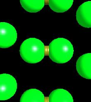
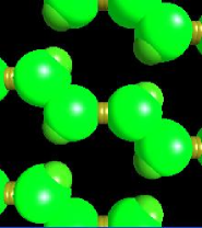
Figure 5. Shown is a picture of ${\mathcal{F}}$ for four geometrically finite structures with long unknotting tunnel. These structures are converging to a structure on ${\partial}GF_{0}(\pi_{1}(C))$. Note that in each of the four structures, the pattern of isometric spheres corresponding to that of Figure 3 is visible, although the number of visible isometric spheres increases.

Let $\phi_{n}$ be any homeomorphism from ${\partial}_{+}C$ to $H$ taking parabolics of $C_{n}$ on ${\partial}_{+}C$ to the parabolics of ${\partial}H$. Because $\phi_{n}$ takes 3–punctured spheres to 3–punctured spheres, it extends to an isometry. Hence we may glue $C_{n}$ to $H$ via $\phi_{n}$ and obtain a tunnel number one manifold with three drilled out curves, corresponding to the three parabolics of ${\partial}_{+}C$. These are three torus boundary components of $M_{n}:=C_{n}\cup_{\phi_{n}}H$.

Select Dehn filling slopes $s^{1}$, $s^{2}$, $s^{3}$ on these three boundary components that act as gluing one boundary to the other by a high power of a Dehn twist. When we Dehn fill along these slopes, the result is a tunnel number one manifold $M_{n}(s^{1},s^{2},s^{3})$. By work of Thurston [19], as the length of the slopes increases, the Dehn filled manifold approaches $M_{n}$ in the geometric topology. Thus the length of the geodesic representative of the homotopy class of the unknotting tunnel in $M_{n}(s^{1},s^{2},s^{3})$ approaches the length of the geodesic representative of the homotopy class of the core tunnel in $C_{n}$ as the lengths of $s^{1}$, $s^{2}$, and $s^{3}$ increase in $M_{n}$.

Hence for large enough $n$ and long enough slopes $s^{1}$, $s^{2}$, $s^{3}$, the Dehn filled manifold $M_{n}(s^{1},s^{2},s^{3})$ is a tunnel number one manifold with unknotting tunnel homotopic to a geodesic of length at least $R$. ∎

4.1. Remarks

While Theorem 4.1 gives us a manifold whose unknotting tunnel has a long geodesic representative, the proof does not guarantee that this tunnel is isotopic to a geodesic, even if we could guarantee that the core tunnel is isotopic to a geodesic in the approximating geometrically finite structures $C_{n}$. This isn’t important for the proof of Theorem 4.1. However, in [11], we will explain how to modify the above proof so that the unknotting tunnel is isotopic to a geodesic.

5. Knots in homology 3-spheres

In this section, we refine the construction in Theorem 4.1 in order to control the homology of the resulting manifolds.

Theorem 5.1.

There exist hyperbolic knots in homology 3-spheres which have tunnel number one, for which the geodesic representative of the unknotting tunnel is arbitrarily long.

The manifolds in the proof of Theorem 4.1 were contructed by starting with maximally cusped geometrically finite uniformizations of the compression body $C$ and the handlebody $H$, gluing them via an isometry, and then performing certain Dehn fillings. We will now vary this construction a little. We will again use maximally cusped geometrically finite uniformizations of the $(1,2)$-compression body $C$ and the genus 2 handlebody $H$, but we will not glue them directly. Instead, we will also find a maximally cusped geometrically finite uniformization of $S\times I$, where $S$ is the closed orientable surface with genus 2, and we will glue $C$ to $S\times\{1\}$ and glue $H$ to $S\times\{0\}$. In both gluings, the parabolic loci will be required to match together, although we will leave these loci unglued. The result is therefore a tunnel number one manifold, with 6 disjoint embedded simple closed curves removed. We will then perform certain Dehn fillings along these 6 curves to give the required tunnel number one manifolds. The choice of hyperbolic structure on $H$ requires some care. In particular we will need the following terminology and results.

Let ${\rm ML}(\partial H)$ (respectively, ${\rm PML}(\partial H)$) be the space of measured laminations (respectively, projective measured laminations) on $\partial H$. (See for example [9]). Let $i(\cdot,\cdot)$ denote the intersection number between measured laminations. A measured lamination $\lambda$ is said to be doubly incompressible if there is an $\epsilon>0$ such that $i(\lambda,\partial E)>\epsilon$ for all essential annuli and discs $E$ properly embedded in $H$. Similarly, a projective measured lamination is doubly incompressible if any of its inverse images in ${\rm ML}(\partial H)$ is doubly incompressible. It is a consequence of Thurston’s geometrization theorem [17] that if $P$ is a collection of simple closed curves on $\partial H$ that are pairwise non-parallel in $\partial H$, essential in $\partial H$ and doubly incompressible, then there is a geometrically finite uniformization of $H$. Let $P$ be the part of its parabolic locus $P$ that lies on $\partial_{+}C$. The set of doubly incompressible projective measured laminations forms a non-empty open subset of ${\rm PML}(\partial H)$ (see [12]).

Lemma 5.2.

There is a homeomorphism $\psi\colon\partial H\rightarrow\partial H$ satisfying the following conditions:

1. $\psi$ is pseudo-Anosov;

2. its stable and unstable laminations are doubly incompressible;

3. the induced homomorphism $\psi_{\ast}\colon H_{1}(\partial H)\rightarrow H_{1}(\partial H)$ is the identity.

Proof.

Since the stable laminations of pseudo-Anosovs are dense in ${\rm PML}(\partial H)$, and the set of doubly incompressible laminations is open and non-empty, there is a pseudo-Anosov homeomorphism $g$ with doubly incompressible stable lamination. Let $h$ be a pseudo-Anosov on $\partial H$ that acts trivially on $H_{1}(\partial H)$ (see [20]). Let $\lambda_{+}$ and $\lambda_{-}$ be its stable and unstable projective measured laminations, which we may assume are distinct from the unstable lamination of $g$. Then the pseudo-Anosov $g^{m}hg^{-m}$ also acts trivially on $H_{1}(\partial H)$. Its stable and unstable laminations are $g^{m}(\lambda_{+})$ and $g^{m}(\lambda_{-})$, which are arbitrarily close to the stable lamination of $g$ for large $m$. Hence, they too are doubly incompressible when $m$ is large. Thus, we may set $\psi$ to be one such $g^{m}hg^{-m}$. ∎

Proof of Theorem 5.1.

Let $\phi\colon\partial_{+}C\rightarrow\partial H$ be a homeomorphism such that, when $C$ is glued to $H$ via $\phi$, the result is the standard genus two Heegaard splitting of the solid torus. Fix a maximally cusped geometrically finite uniformization of $C$ from the proof of Theorem 4.1, for which the core tunnel has long geodesic representative. Let $P$ be its parabolic locus. Then $\phi(P)$ is a collection of simple closed curves on $H$.

Let $\tau$ be a composition of Dehn twists, one twist around each component of $\phi(P)$. Let $\psi$ be the pseudo-Anosov homeomorphism provided by Lemma 5.2. By replacing $\psi$ by a power of $\psi$ if necessary, we may assume that for each core curve $\alpha$ of $P$, $i(\alpha,\psi(\alpha))\not=0$. The tunnel number one manifold that we are aiming for is obtained by gluing $C$ to $H$ via $\psi^{m}\tau^{-M}\psi^{-1}\tau^{M}\phi$ for large integers $m$ and $M$. Since $\psi$ acts trivially on homology, this has the same homology as if we had glued by $\phi$, which gives the solid torus. Thus, this manifold is indeed the exterior of a knot in a homology 3-sphere.

We first choose the integer $m$. As $m$ tends to infinity, $\psi^{m}\phi(P)$ tends to the stable lamination of $\psi$ in ${\rm PML}(\partial H)$. Hence, we may choose such an $m$ so that $\psi^{m}\phi(P)$ is doubly incompressible.

We start with three manifolds:

1. $C-P$;

2. $(S\times[0,1])-((\phi(P)\times\{1\})\cup(\psi\phi(P)\times\{0\}))$;

3. $H-\psi^{m}\phi(P)$.

Here, $S$ is the genus two surface, which we identify with $\partial H$. The second of the above manifolds has a geometrically finite uniformization, by Thurston’s geometrization theorem. This because any essential annulus in $S\times[0,1]$ with boundary in $(\phi(P)\times\{1\})\cup(\psi\phi(P)\times\{0\})$ can be homotoped, relative to its boundary, so that it lies entirely in $(\phi(P)\times\{1\})\cup(\psi\phi(P)\times\{0\})$. Similarly, because $\psi^{m}\phi(P)$ is doubly incompressible, $H-\psi^{m}\phi(P)$ admits a geometrically finite hyperbolic structure. Glue $C-P$ to $(S-\phi(P))\times\{1\}$ via $\phi$, and glue $(S-\psi\phi(P))\times\{0\}$ to $H-\psi^{m}\phi(P)$ via $\psi^{m-1}$. Since these manifolds have conformal boundary that consists of 3-punctured spheres, this gluing can be performed isometrically.

As in the proof of Theorem 4.1, we now perform certain Dehn fillings on the toral cusps of this manifold, apart from the cusp corresponding to $\partial_{-}C$. If the Dehn filling is done correctly, this has the effect of modifying the gluing map by powers of Dehn twists. We may apply any iterate of these Dehn twists, and so we apply the $M$th iterate, where $M$ is some large positive integer, along each of the curves $\phi(P)\times\{1\}$ in $S\times\{1\}$ and the $(-M)$th power along each of the curves in $\psi\phi(P)\times\{0\}$ in $S\times\{0\}$. Thus, the gluing map becomes $\psi^{m}\tau^{-M}\psi^{-1}\tau^{M}\phi$. As $M$ tends to infinity, these manifolds tend geometrically to the unfilled manifold. In particular, for large $M$, the geodesic representative of its unknotting tunnel will be long. ∎

6. The Dehn filling construction

In this section, we give the proof of Theorem 4.1 that uses Dehn filling and homology.

Let $X$ be a compact $3$–manifold with four torus boundary components and of Heegaard genus $2$. This means there is a closed genus $2$ surface $F$ in the interior of $X$ which separates $X$ into two compression bodies, each homeomorphic to the manifold $V$ obtained by adding one $2$–handle onto a copy of $F\times[0,1]$ along an essential separating simple closed curve in $F\times\{1\}.$ We label the torus boundary components of $X$ by $A_{0}$, $A_{1}$, $B_{0}$, $B_{1}$ so that $A_{0}$ and $B_{0}$ are on the same side of $F$.

Let $\beta_{0}$, $\beta_{1}$, and $\alpha_{1}$ be essential simple closed curves on $B_{0}$, $B_{1}$, and $A_{1}$, respectively. Let $M=X(\alpha_{1},\beta_{0},\beta_{1})$ be the manifold obtained by Dehn filling using these slopes, so that $M$ has a single boundary component $A_{0}.$ Gluing a solid torus to each of the two boundary components of $V$ yields a genus $2$ handlebody. It follows that $M$ has tunnel number one; indeed a tunnel is obtained using an arc with endpoints on $A_{0}$ that goes round the core of the solid torus used to fill along $B_{0}$.

Lemma 6.1.

There exists $X$ as above such that the interior of $X$ admits a complete hyperbolic structure of finite volume, such that $H_{1}(X)\cong\Gamma_{A}\oplus\Gamma_{B}$ where $\Gamma_{A}\cong\Gamma_{B}\cong{\mathbb{Z}}^{2}$, and under maps induced by inclusion, $H_{1}(A_{i})=\Gamma_{A}$ and $H_{1}(B_{i})=\Gamma_{B}$ for $i=1,2.$

Proof.

An example of $X$ is provided by the exterior of the $4$ component link $L$ in $S^{3}$ shown in Figure 6. The link $L=a_{0}\cup a_{1}\cup b_{0}\cup b_{1}$ consists of two linked copies of the Whitehead link and is hyperbolic (by SnapPea [21]). Furthermore $Lk(a_{0},a_{1})=Lk(b_{0},b_{1})=1$ and $Lk(a_{i},b_{j})=0$. The diagram also shows disjoint arcs $\alpha$ connecting $a_{0}$ to $b_{0}$ and $\beta$ connecting $a_{1}$ to $b_{1}$. It is easy to slide these arcs and links in such a way that the pair of graphs $a_{0}\cup b_{0}\cup\alpha$ and $a_{1}\cup b_{1}\cup\beta$ are spines of the handlebodies of the genus $2$ Heegaard spliting of $S^{3}$. It follows that $X=S^{3}-{\eta}(L)$ has the required properties and $A_{i}=\partial\eta(a_{i})$ and $B_{i}=\partial\eta(b_{i})$. Here $\eta(L)$ denotes an open tubular neighborhood of $L$. ∎

Figure 6. A hyperbolic link satisfying the conditions of Lemma 6.1.

Suppose $X$ is a link of Lemma 6.1. Let $x$ be a basepoint for $X$ on the boundary of a maximal horoball neighborhood of the cusp corresponding to $A_{0}$. The idea for finding the Dehn fillings to give $M$ is that given a base point $x$ in $X$ and $R>0$, there are only finitely many homotopy classes of loops in $X$ based at $x$ with length at most $3R$. These give finitely many classes in $H_{1}(X)$ and hence, under projection, finitely many classes $\gamma_{1},\cdots\gamma_{p}\in\Gamma_{B}$. The Dehn fillings used to obtain $M$ are chosen so that $H_{1}(M)\cong{\mathbb{Z}}\oplus{\mathbb{Z}}_{n}$ with the image of $\Gamma_{B}$ being ${\mathbb{Z}}_{n}$ and that of $\Gamma_{A}$ being ${\mathbb{Z}}$. The fillings are also chosen so that none of the images of $\gamma_{i}$ generate ${\mathbb{Z}}_{n}$, and so that the hyperbolic metric on $M$ is geometrically close to that of $X$. In particular, we may assume that there is a bilipschitz homeomorphism, with bilipschitz constant very close to $1$, between the $R$ neighborhood of the basepoint of $x$ in $X$ and a subset of $M$. Let $m$ be the image of $x$ in $M$, which we may assume lies on the boundary of a maximal horoball neighborhood of the cusp of $M$. Then every loop in $M$ based at $m$ of length at most $2R$ corresponds to a loop in $X$ based at $x$ with length at most $3R$, say.

Lemma 6.2.

Suppose $\Gamma$ is a free abelian group of rank $2$ and $\gamma_{1},\cdots\gamma_{p}\in\Gamma$. Then there is an integer $n>0$ and an epimorphism $\phi_{n}\colon\thinspace\Gamma\rightarrow{\mathbb{Z}}_{n}$ such that for all $i$ the element $\phi_{n}(\gamma_{i})$ does not generate ${\mathbb{Z}}_{n}$.

Proof.

Clearly we may assume that for all $i$, $\gamma_{i}\neq 0$. Then we may identify $\Gamma$ with ${\mathbb{Z}}^{2}$ so that $\gamma_{i}=(a_{i},b_{i})$ and for all $i$, $a_{i}\neq 0$. Set $m=\max_{i}|b_{i}|+2$ and define a homomorphism $\phi\colon\thinspace{\mathbb{Z}}^{2}\rightarrow{\mathbb{Z}}$ by $\phi((a,b))=2ma-b$ which is surjective because $\phi((1,2m-1))=1$. Set $c_{i}=|\phi(\gamma_{i})|$. Then c_i = —2ma_i-b_i— ≥2m—a_i—-—b_i— ≥2m-m ≥2, using that $|a_{i}|\geq 1$ and $|b_{i}|\leq m$ and $m\geq 2$. Now define $n=\prod_{i}c_{i}$ and define $\phi_{n}(\gamma)=\phi(\gamma)$ mod $n$. Then $\phi_{n}(\gamma_{i})=\pm c_{i}$ and $c_{i}\neq 1$ divides $n$ and therefore does not generate ${\mathbb{Z}}_{n}.$ ∎

For the Dehn fillings of $B_{0}$ and $B_{1}$, choose simple closed curves $\beta_{i}\subset B_{i}$ which generate the kernel of ϕ_n: Γ_B →Z_n, where here we are using the identifications $H_{1}(B_{0})\equiv\Gamma_{B}\equiv H_{1}(B_{1})$. There are arbitrarily large pairs of such basis elements; thus we may choose them so that the result of hyperbolic Dehn filling $B_{0}$ and $B_{1}$ using these gives a two cusped hyperbolic manifold with metric on the thick part as close to that of $X$ as desired.

Now perform a very large Dehn filling (thus not distorting the geometry of the thick part appreciably) along $A_{1}$. We claim we obtain $M$ with all the required properties.

For suppose that the geodesic representative for the unknotting tunnel of $M$ had length at most $R$. Let $T$ be the torus that forms the boundary of a maximal horoball neighborhood of the cusp of $M$. The basepoint $m$ of $M$ lies on $T$. We may pick $R$ large enough so that $\pi_{1}(T,m)$ is generated by two curves of length at most $R$. In addition, the geodesic representative for the unknotting tunnel can be closed up to form a loop based at $m$ with length at most $2R$. These three loops generate $\pi_{1}(M,m)$. By construction, $H_{1}(M)\cong{\mathbb{Z}}\oplus{\mathbb{Z}}_{n}$. The image of $H_{1}(T)$ in $H_{1}(M)$ is the first summand, and the image of the third loop is a proper subgroup of the second summand. Thus, these three loops cannot generate $H_{1}(M)$, which is a contradiction. Hence, the geodesic representative for the unknotting tunnel of $M$ has length more than $R$. Since $R$ was arbitrarily large, this establishes Theorem 4.1.

References

- [1] Colin Adams, Unknotting tunnels in hyperbolic -manifolds, Math. Ann. 302 (1995), no. 1, 177–195.
- [2] Colin C. Adams and Alan W. Reid, Unknotting tunnels in two-bridge knot and link complements, Comment. Math. Helv. 71 (1996), no. 4, 617–627.
- [3] Hirotaka Akiyoshi, Yoshiyuki Nakagawa, and Makoto Sakuma, Shortest vertical geodesics of manifolds obtained by hyperbolic Dehn surgery on the Whitehead link, KNOTS ’96 (Tokyo), World Sci. Publ., River Edge, NJ, 1997, pp. 433–448.
- [4] Lipman Bers, On moduli of Kleinian groups, Russ. Math. Surv. 29 (1974), 88–102.
- [5] B. H. Bowditch, Geometrical finiteness for hyperbolic groups, J. Funct. Anal. 113 (1993), no. 2, 245–317.
- [6] Richard D. Canary, Marc Culler, Sa’ar Hersonsky, and Peter B. Shalen, Approximation by maximal cusps in boundaries of deformation spaces of Kleinian groups, J. Differential Geom. 64 (2003), no. 1, 57–109.
- [7] Marc Culler and Peter B. Shalen, Varieties of group representations and splittings of -manifolds, Ann. of Math. (2) 117 (1983), no. 1, 109–146.
- [8] D. B. A. Epstein and R. C. Penner, Euclidean decompositions of noncompact hyperbolic manifolds, J. Differential Geom. 27 (1988), no. 1, 67–80.
- [9] A. Fathi, F. Laudenbach, and V. Poenaru, Travaux de Thurston sur les surfaces, Astérisque, vol. 66, Société Mathématique de France, Paris, 1979, Séminaire Orsay, With an English summary.
- [10] Daniel J. Heath and Hyun-Jong Song, Unknotting tunnels for , J. Knot Theory Ramifications 14 (2005), no. 8, 1077–1085.
- [11] Marc Lackenby and Jessica S. Purcell, Geodesic arcs in compression bodies, In preparation.
- [12] Cyril Lecuire, An extension of the Masur domain, preprint.
- [13] Albert Marden, The geometry of finitely generated kleinian groups, Ann. of Math. (2) 99 (1974), 383–462.
- [14] by same author, Outer circles, Cambridge University Press, Cambridge, 2007, An introduction to hyperbolic 3-manifolds.
- [15] Bernard Maskit, Kleinian groups, Grundlehren der Mathematischen Wissenschaften [Fundamental Principles of Mathematical Sciences], vol. 287, Springer-Verlag, Berlin, 1988.
- [16] Curt McMullen, Cusps are dense, Ann. of Math. (2) 133 (1991), no. 1, 217–247.
- [17] John W. Morgan and Hyman Bass (eds.), The Smith conjecture, Pure and Applied Mathematics, vol. 112, Academic Press Inc., Orlando, FL, 1984, Papers presented at the symposium held at Columbia University, New York, 1979.
- [18] Makoto Sakuma and Jeffrey Weeks, Examples of canonical decompositions of hyperbolic link complements, Japan. J. Math. (N.S.) 21 (1995), no. 2, 393–439.
- [19] William P. Thurston, The geometry and topology of three-manifolds, Princeton Univ. Math. Dept. Notes, 1979.
- [20] by same author, On the geometry and dynamics of diffeomorphisms of surfaces, Bull. Amer. Math. Soc. (N.S.) 19 (1988), no. 2, 417–431.
- [21] Jeffrey Weeks, Snappea, Available at http://www.geometrygames.org/SnapPea/.