Double Pair Production by Ultra High Energy Cosmic Ray Photons

Abstract

With use of CompHEP package we’ve made the detailed estimate of the influence of double $e^{+}e^{-}$ pair production (DPP) by photons on the propagation of ultra high energy electromagnetic (EM) cascade. We show that in the models in which cosmic ray photons energy reaches few$\times 10^{3}$ EeV refined DPP analysis may lead to substantial difference in predicted photon spectrum compared to previous rough estimates.

1 Introduction

Ultra-high energy (UHE) photons have not been recognized so far by any of present generation experiments [1, 2, 3, 4], although their existence is predicted by Greisen–Zatsepin–Kuzmin effect [5, 6] as well as by most of hypothetical top-down models of UHE cosmic rays origin. There are several bounds on fraction and flux of ultra-high energy photons above $10-100\,{\rm EeV}$ obtained by independent experiments [7, 8, 9]. Photon limits are used to constrain the parameters of top-down models (see for example [10]). Future bounds may also limit considerable part of parameter space of astrophysical models, in which photons are produced as secondaries from interactions of primary protons or nuclei with cosmic microwave background (CMB). Understanding interactions of UHE photons with universal backgrounds is a crucial point for building such constraints.

In the wide energy range the spectra of electron and photon components of cosmic rays follow each other due to relatively rapid processes transferring $\gamma$-rays to electrons and backwards. Pair production (PP) and inverse Compton scattering (ICS) are the main processes that drive the EM cascade. In the Klein–Nishina limit where $s\gg m_{e}^{2}$, either electron or positron produced in a pair production event typically carries almost all of the initial total energy. The produced electron (positron) then undergoes ICS losing more than 90 % of energy and finally the background photon carries away almost all of the initial energy of the UHE photon. Due to this cycle the energy loss rate of the leading particle in the EM cascade is more than one order of magnitude less than interaction rate. However in presence of a random extragalactic magnetic field (EGMF) the electrons may lose substantial part of their energy by emitting synchrotron radiation. In this case, starting from certain energy the synchrotron loss rate for the electrons becomes to dominate over ICS rate, which leads to suppression of the EM cascade development. Its penetration depth is then defined by the photon mean free path. Depending on the value of EGMF this transition may occur between $\sim 1\,{\rm EeV}$ and $\sim 10^{6}\,{\rm EeV}$.

In this article we consider higher order process, double $e^{+}e^{-}$ pair production (DPP) by photons. The DPP cross section grows rapidly with $s$ near the threshold and quickly approaches the asymptotic value $\sigma(\infty)\simeq 6.45~{}\,{\rm\mu{b}}$ [11, 12, 13]. The explicit energy dependence of the DPP cross section was estimated in Ref. [14] by calculating the dominant contribution from two $e^{+}e^{-}$ pairs to the absorptive part of gamma-gamma forward scattering amplitude. Since PP cross section decreases with the increase of $\sqrt{s}$ the DPP rate starts to dominate over PP rate above certain energy. For interactions with CMB the transition occurs above $\sim 1000\,{\rm EeV}$. In presence of the radio background this energy goes up somewhat. If the EGMF is less than $10^{-11}\,{\rm G}$ the EM cascade still exists at these energies and one should accurately count the secondary electrons from DPP. So far the EM cascade simulations such as [15, 16] roughly estimated DPP effect by utilizing the total cross section and assuming that one $e^{+}e^{-}$ pair of the two carries all the initial energy while two particles in the pair are produced with the same energy. By making use of CompHEP package [17, 18, 19] we numerically calculate differential cross section for DPP and compare the influence of DPP on propagation of ultra high energy EM cascade with previous estimates.

The paper is organized as follows. In Sec. 2 we present the results of the calculation of DPP cross section. In Sec. 3 we write transport equations for EM cascade and calculate the coefficients for transport equations for photons, and secondary $e^{+}$,$e^{-}$ related to DPP. In Sec. 4 we illustrate the influence of DPP in model example. In Sec. 5 we summarize our results.

2 DPP cross section calculation

As it was mentioned in the Introduction the DPP process begins to dominate over PP at very high energies $E_{\gamma}\mathrel{\mathchoice{\lower 3.6pt\vbox{\halign{$\mathsurround=0pt\displaystyle\hfil#\hfil$\cr>\crcr\sim\crcr}}}{\lower 3.6pt\vbox{\halign{$\mathsurround=0pt\textstyle\hfil#\hfil$\cr>\crcr\sim\crcr}}}{\lower 3.6pt\vbox{\halign{$\mathsurround=0pt\scriptstyle\hfil#\hfil$\cr>\crcr\sim\crcr}}}{\lower 3.6pt\vbox{\halign{$\mathsurround=0pt\scriptscriptstyle\hfil#\hfil$\cr>\crcr\sim\crcr}}}}1000$ EeV or $s\mathrel{\mathchoice{\lower 3.6pt\vbox{\halign{$\mathsurround=0pt\displaystyle\hfil#\hfil$\cr>\crcr\sim\crcr}}}{\lower 3.6pt\vbox{\halign{$\mathsurround=0pt\textstyle\hfil#\hfil$\cr>\crcr\sim\crcr}}}{\lower 3.6pt\vbox{\halign{$\mathsurround=0pt\scriptstyle\hfil#\hfil$\cr>\crcr\sim\crcr}}}{\lower 3.6pt\vbox{\halign{$\mathsurround=0pt\scriptscriptstyle\hfil#\hfil$\cr>\crcr\sim\crcr}}}}1$ ${\rm GeV}^{2}$, which is well beyond the DPP threshold. At these and higher energies DPP has noticeable effect on the propagation of EM cascade. In this energy region DPP total cross section is practically saturated by its asymptotic value. So, we are interested here mostly in energy and angular distributions of secondary electrons (positrons) in asymptotic regime ($s\to\infty$).

We use CompHEP package for calculation of tree level differential DPP cross sections. This package allows to perform automatic calculations of matrix elements and their squares for any process $2\to 2$, .., $2\to 4$ at tree level. Then, with the aid of CompHEP one can integrate squared matrix elements over selected part of multi-particle phase space. See Refs. [17, 18, 19] for the details.

We introduce binning in the energy $E^{*}$ of one of the produced electrons. Then we perform CompHEP simulations in the centre of mass frame (CMF) and obtain distributions over $\cos{\Theta^{*}}$ of the cross section in a given energy bin. Here $\Theta^{*}$ is the angle between the collision axis and the momentum vector of the electron.

These calculations show that the angular distribution of secondaries tends to a strongly peaked function of $\cos{\Theta^{*}}$ in the asymptotic energy range. The peaks are located at forward and backward directions, i.e. at $\cos{\Theta^{*}}=\pm 1$. This behavior is illustrated by Fig. 1

Figure 1: Example of distribution of the DPP cross sections over $\cos{\Theta^{*}}$ for $\sqrt{s}=10.0$ GeV in energy $E^{*}$ bin $2.25-2.5$ GeV.

where we show an example of angular distribution for $\sqrt{s}=10.0$ GeV. The effect that most of secondaries go forward or backward becomes more pronounced with the increase of $\sqrt{s}$ and in the case of fixed $\sqrt{s}$ with higher energy $E^{*}$ of electron. Numerically we found that the probability of emitting secondary electron inside the cone with $\mid 1-\cos{\Theta^{*}}\mid<1/50$ is 96.8% for $\sqrt{s}=1.0$ GeV, 98.7% for $\sqrt{s}=2.5$ GeV and 99.6% for $\sqrt{s}=10.0$ GeV. Also we checked that the probability of producing two forward secondaries of the same type (e.g., when both forward particles are electrons) integrated over energies and directions of other secondaries, is of order $10^{-3}$. So, the main part of events consists of two $e^{+}e^{-}$ pairs going to the opposite directions along the collision axis.

Let us now turn to the energy distribution. It is clear from the symmetry of the problem that the energy distribution in the CMF frame should be the same for the forward and backward electrons. Let us write the DPP differential cross section in the form

$$\frac{d\sigma}{dE^{*}}\equiv\frac{1}{\sqrt{s}}\phi\left(\frac{E^{*}}{\sqrt{s}/2},s\right)\sigma_{tot}(s)\;.$$ (1)

Then the energy conservation condition gives

$$\sqrt{s}\sigma_{tot}(s)=4\int_{0}^{\sqrt{s}/2}E^{*}\frac{d\sigma}{dE^{*}}\,dE^{*}=\sigma_{tot}(s)\,\sqrt{s}\int_{0}^{1}r\phi(r,s)\,dr$$

or for any value of $s$

$$\int_{0}^{1}r\phi(r,s)\,dr=1\;.$$ (2)

Imposing probability conservation requirement

$$\sigma_{tot}(s)=\int_{0}^{\sqrt{s}/2}\frac{d\sigma}{dE^{*}}\,dE^{*}$$

gives another integral constraint on $\phi(r,s)$:

$$\int_{0}^{1}\phi(r,s)\,dr=2\;.$$ (3)

Although conditions (2) and (3) do not necessary imply ${d\phi}/{ds}=0$ the results of CompHEP simulations show that for large enough $s$, when cross section approaches its asymptotic value, the energy distribution of secondaries in units of maximal energy $\sqrt{s}/2$ varies only slightly with $\sqrt{s}$. In Fig. 2

Figure 2: The normalized energy distributions $\phi(r,s)$, $r=2E^{*}/\sqrt{s}$ (see main text for details): 1) $\sqrt{s}$ = $0.1$ GeV, 2) $\sqrt{s}$ = $0.25$ GeV, 3) $\sqrt{s}$ = $10.0$ GeV and 4) the analytic approximation Eq. (4).

we plot the distribution $\phi(r,s)$ as a function of $r$ for different values of $\sqrt{s}$. One can see that with varying $\sqrt{s}$ the only changes in these distributions are concentrated at the borders of the plot. The distribution limit for $s\to\infty$ can be fitted (see fig. 2) by simple analytic expression, which satisfies constraints (2) and (3),

$$\phi_{fit}(r)=\frac{5}{3}+(2r-1)^{2}.$$ (4)

For comparison, the earlier approximation [15, 16] in terms of the distribution $\phi(r,s)$ reads

$$\phi(r,s)=2\cdot\delta(r-0.5).$$ (5)

In our further calculations we use for the energy distribution the Eq. (1), where $\phi(r,s)=\phi_{fit}(r)$ is given by Eq. (4) and assume that all the secondary particles are directed alongside the collision axis. In Sec. 4 we discuss how good the above approximation is.

3 Transport Equations

Here we describe propagation of the UHE cosmic rays using the formalism of transport equations in one dimension. Besides DPP term on which we are going to focus now, the full transport equations for the electrons and photons contain the terms describing ICS, PP, synchrotron and $e^{+}e^{-}$ pair production by electrons and positrons as well as redshift terms. For simplicity, we show below the part of the equation written for nonexpanding universe with the terms related to the DPP process only.

$$\frac{d}{dt}N_{e}(E_{e},t)=\int_{E_{e}}^{\infty}dE_{\gamma}N_{\gamma}(E_{\gamma},t)\int_{\epsilon_{min}}^{\epsilon_{max}}d\epsilon\,n(\epsilon)\int_{-1}^{1}d\mu\frac{1-\mu}{2}\frac{d\sigma_{\rm DPP}}{dE_{e}}(E_{e},E_{\gamma},s)\,$$ (6)

$$\frac{d}{dt}N_{\gamma}(E_{\gamma},t)=-N_{\gamma}(E_{\gamma},t)\int_{\epsilon_{min}}^{\epsilon_{max}}d\epsilon\,n(\epsilon)\int_{-1}^{1}d\mu\frac{1-\mu}{2}\sigma_{\rm DPP}(s)$$ (7)

where $N_{e}(E_{e},t)$ is the (differential) number density of electrons at energy $E_{e}$ at time $t$, $n(\epsilon)$ is the number density of background photons at energy $\epsilon$, $\mu$ is the cosine of the collision angle ($\mu=-1$ for a head-on collision) and $s=2E_{\gamma}\epsilon(1-\mu)$ is center of mass energy squared. The term in the r.h.s. part of Eq. (6) describes influx of electrons produced in DPP. Transport equation for positrons has the same form as (6). The r.h.s. term of (7) describes the loss of photons due to DPP. The factor $(1-\mu)/2$ is the flux factor. As we’ve seen in the Sec. 2 the pairs produced in DPP are directed alongside the collision axis. This implies that one of the pairs carries practically all the initial energy of the photon in the laboratory frame. Here we neglect the nonleading pair produced in the interaction.

Replacing integration over $\mu$ by integration over $s$ gives

$$\frac{d}{dt}N_{e}(E_{e},t) = \int_{E_{e}}^{\infty}dE_{\gamma}\frac{N_{\gamma}(E_{\gamma},t)}{8E_{\gamma}^{2}}\int_{s_{th}}^{s_{max}}ds\,s\frac{d\sigma_{\rm DPP}}{dE_{e}}(E_{e};E_{\gamma},s)I_{\epsilon}(\frac{s}{4E_{\gamma}}),$$ (8)

$$\frac{d}{dt}N_{\gamma}(E_{\gamma},t) = -\frac{N_{\gamma}(E_{\gamma},t)}{8E_{\gamma}^{2}}\int_{s_{th}}^{s_{max}}ds\,s\,\sigma_{\rm DPP}(s)I_{\epsilon}(\frac{s}{4E_{\gamma}})$$ (9)

where

$$I_{\epsilon}(x)=\int_{x}^{\epsilon_{max}}\frac{n(\epsilon)}{\epsilon^{2}}d\epsilon\;.$$ (10)

Here $s_{th}=16m_{e}^{2}$ is threshold CMF energy squared for DPP and $s_{max}=4E_{\gamma}\epsilon_{max}$.

Now we are ready to use the results obtained in the Sec. 2. Again here we calculate the transport equation coefficients in the limit of $s{\gg}s_{th}$. This implies that electrons and positrons are ultrarelativistic in the CMF frame. The CMF $\gamma$-factor in the laboratory frame is

$$\gamma_{CMF}\equiv(1-\beta_{CMF}^{2})^{-\frac{1}{2}}=\frac{E_{\gamma}}{\sqrt{s}}\;.$$

Provided that $e^{+}$ and $e^{-}$ momenta are directed either towards the CMF frame velocity or in the opposite direction, their energy in the laboratory frame

$$E_{e}=\gamma_{CMF}E_{e}^{*}(1\pm\beta_{e}^{*})=\frac{E_{\gamma}}{\sqrt{s}}E_{e}^{*}(1\pm\beta_{e}^{*}),$$

where $\beta_{e}^{*}\rightarrow 1$ is electron velocity in CMF. For the leading $e^{+}e^{-}$ pair we have:

$$E_{e}=2\frac{E_{\gamma}}{\sqrt{s}}E_{e}^{*}\;.$$

Then using Eq. (1) we finally obtain

$$\frac{d}{dt}N_{e}(E_{e},t)=\frac{1}{16}\int_{E_{e}}^{\infty}dE_{\gamma}\frac{N_{\gamma}(E_{\gamma},t)}{E_{\gamma}^{3}}\phi(\frac{E_{e}}{E_{\gamma}})\int_{s_{th}}^{s_{max}}ds\,s\,\sigma_{\rm DPP}(s)I_{\epsilon}(\frac{s}{4E_{\gamma}})\;.$$ (11)

Using numerical simulations of cosmic rays propagation presented in the Sec. 4 we have also verified that utilizing simple step function for the total cross section

$$\sigma_{\rm DPP}(s)=\sigma_{\rm DPP}(\infty)\Theta(s-s_{th})$$ (12)

instead of exact one listed in [14], doesn’t introduce any visible change to the resulting spectra. This implies that the equations (11) and (9) can be simplified as follows:

$$\frac{d}{dt}N_{e}(E_{e},t)\simeq\sigma_{\rm DPP}(\infty)\int_{E_{e}}^{\infty}dE_{\gamma}\frac{N_{\gamma}(E_{\gamma},t)}{E_{\gamma}}\phi(\frac{E_{e}}{E_{\gamma}})K_{\epsilon}(s_{th}/4E_{\gamma}),$$ (13)

$$\frac{d}{dt}N_{\gamma}(E_{\gamma},t)\simeq-2\sigma_{\rm DPP}(\infty)N_{\gamma}(E_{\gamma},t)K_{\epsilon}(s_{th}/4E_{\gamma}),$$ (14)

where

$$K_{\epsilon}(x)=\int_{x}^{\epsilon_{max}}I_{\epsilon}(y)y\,dy$$ (15)

is the function totally determined by the background photons spectrum.

4 Model example

In the previous sections we have found the precise expression for the distribution of secondary electrons from DPP. Here we consider a model example to illustrate the difference introduced by the specified cross section compared to the previous estimates.

We use a numerical code developed in Ref. [15] to compute the flux of produced photons and protons. The code is based on the transport equations and calculates the propagation of nucleons, electrons and photons using the dominant processes. For EM cascade it includes all the processes mentioned above. For nucleons, it takes into account single and multiple pion production and $e^{+}e^{-}$ pair production, neutron $\beta$-decay. The propagation of nucleons and the EM cascades are calculated self-consistently, that is secondary particles produced in all reactions are propagated alongside the primaries.

Besides CMB the radio, infra-red and optical (IRO) components of the universal photon background are taken into account in the simulation. Note that the radio background is not yet well known. Our results will depend strongly on the radio background assumed. Three models considered in this work are estimates by Clark et al. [20] and the two models of Protheroe and Biermann [21], both predicting larger background than the first one. For the IRO background component we used the model [22]. This component doesn’t have substantial effect on the propagation of UHE protons and EM cascade. For the strength of the random extragalactic magnetic field we use the range of values $10^{-12}{\rm G}<B<10^{-11}{\rm G}$ following the estimate [23].

Among the models we have chosen the one in which the UHE photons contribute substantial part of the total spectrum. Note that such models are strictly limited by the present experimental bounds on the photon component, see [10] for details.

Figure 3: Fluxes predicted by proton emitting source described in text. The dotted line represents proton component, while solid, dashed and dash-dotted lines represent total flux calculated with CompHEP based DPP, trivial DPP estimate and without DPP correspondingly.

In Fig. 3 the propagated cosmic ray flux is shown for proton sources with spectrum

$$\frac{d\Phi}{dE}\sim E^{-1.5},\,\,E<10^{4}{\rm EeV}\$$ (16)

homogeneously distributed in the Universe and having no evolution in the comoving frame. The spectrum presented is normalized on HiRes [3] results (fitting was done above $40\,{\rm EeV}$). The solid line represents the total UHE cosmic ray flux calculated with use of new DPP estimate. The dotted line shows proton component. The dashed line shows total flux calculated using earlier DPP estimate (Eq. 5), utilizing the total cross section and assuming that one $e^{+}e^{-}$ pair of the two carries all the initial energy while two particles in the pair are produced with the same energy. The dash-dotted lines are built without taking DPP into account at all.

It is clear from the Fig. 3 that DPP suppresses $\gamma$ ray flux above $100\,{\rm EeV}$. This is only true if the minimal radio background model [20] is used. The same picture made for any of the two models of [21] haven’t shown any effect of DPP, since in this case the $\gamma$ flux is strongly suppressed by PP on radio. Increasing magnetic field above $10^{-11}{\rm G}$ also destroys the picture, this time due to synchrotron radiation. In the case of minimal radio background and moderate EGMF the trivial DPP effect estimate leads to extra suppression compared to the more accurate one proposed in this paper. Although overall error in terms of integral photon flux above $100\,{\rm EeV}$ turns to be only $+7$% for the curve disregarding DPP and just $-1.5$% for the trivial DPP estimate. Note that integral photon flux fraction predicted in this model is 34%, which is very close to the upper bound [7].

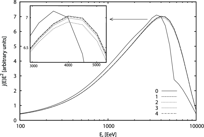
Figure 4: Electron flux predicted by photon emitting source described in text using 0) earlier estimate Eq. (5); 1) analytical fit (4); 2) analytical fit (4) + 3.2% perpendicular component (see details in text); 3) $\phi(r,1\,{\rm GeV}^{2})$; 4) $\phi(r,100\,{\rm GeV}^{2})$.

So far we used the fixed energy distribution (4) for all values of $s$. Also we assumed that all the secondary particles are directed alongside the collision axis. Let us now check how accurate the above approximations are. We have repeated our simulations replacing the energy distribution (4) by the tabulated functions obtained with use of CompHEP for $\sqrt{s}=1\,{\rm GeV}$ and $\sqrt{s}=10\,{\rm GeV}$. To see the maximal possible effect of the nontrivial angular distribution of secondaries we have also repeated our calculations assuming that 3.2% of secondary particles are aligned perpendicular to the collision axis in the CMF, while the rest of the particles are directed alongside the axis. We don’t show here the modified fluxes obtained in the model corresponding to Fig. 3, since they are practically indistinguishable from the curves already shown. Instead to illustrate the maximal possible error introduced by the approximation used, here we consider the pure photon sources with the same injection spectrum (16) as in Fig. 3 and count the income to the propagated electron and photon spectra from the uniformly distributed sources located within $500\,{\rm Mpc}$ from the observer. In Figs. 4 and 5 the electron and photon fluxes in this model are shown respectively.

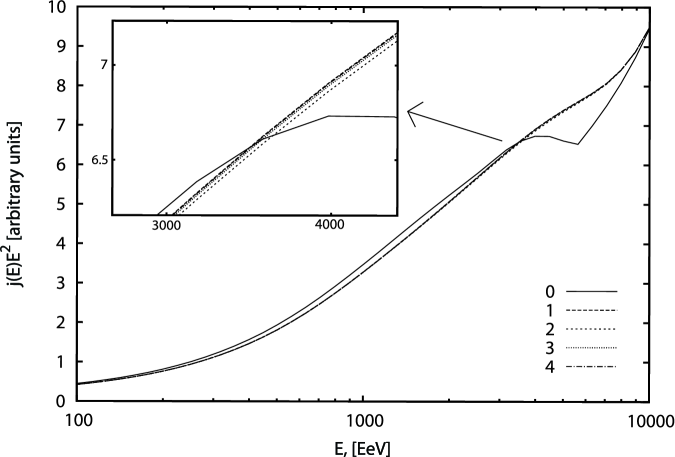
Figure 5: Propagated photons flux predicted by photon emitting source described in text. The designation of curves is the same as on Fig. 4.

Also on these figures the fluxes calculated using earlier estimate Eq. (5) are shown. From the figures it is clear that the earlier estimate may lead to the artificial features in the spectra which doesn’t appear in our analysis. Also it is clear that discrepancy between the curves 1-4 representing different variants of our analysis are small compared to the error introduced by the earlier estimate. In fact the difference between the curves 1-4 is comparable to the error introduced by finite energy binning used in our numerical code.

5 Conclusion

In this work we have considered in detail the DPP process. We have estimated the distribution of secondary electrons and positrons and made the improved cosmic rays simulation based on the new estimate. We have shown that in certain cases the DPP process may modify the photon component of the spectrum substantially. However this modification can only be seen if radio background is close to the minimal model [20] and EGMF is lower than $10^{-11}{\rm G}$. In this case there is an energy range where DPP is the main attenuation mechanism for $\gamma$ rays and therefore differences in DPP estimates can clearly be seen. Although in the vast majority of the models which do not contradict to the present experimental bounds on the photon fraction in UHE cosmic rays DPP process doesn’t make a substantial contribution to the attenuation and therefore can be treated simplistically or even disregarded.

We are indebted to D. Gorbunov for inspiring us to prepare this work. We also thank D. Semikoz for valuable discussions. This work was supported in part by the Russian Foundation of Basic Research grant 07-02-00820, by the grant of the President of the Russian Federation NS-1616.2008.2, MK-1966.2008.2 (O.K.). Work of S.D. was supported in part by the grant of the Russian Science Support Foundation, Russian Foundation of Basic Research grants 08-02-00473-a and 08-02-00768-a. Numerical part of the work was performed on the Computational cluster of the Theoretical Division of INR RAS.

References

- [1] M. Takeda et al., Astropart. Phys. 19, 447 (2003) [arXiv:astro-ph/0209422].
- [2] V. P. Egorova et al., Nucl. Phys. Proc. Suppl. 136, 3 (2004) [arXiv:astro-ph/0408493].
- [3] R. U. Abbasi et al. [High Resolution Fly’s Eye Collaboration], Phys. Rev. Lett. 92, 151101 (2004) [arXiv:astro-ph/0208243].
- [4] J. Abraham et al. [Pierre Auger Collaboration], Phys. Rev. Lett. 101, 061101 (2008) [arXiv:0806.4302 [astro-ph]].
- [5] K. Griesen, Phys. Rev. Lett. 16, 748 (1966)
- [6] Z. T. Zatsepin and V. A. Kuz’min, Zh. Eksp. Teor. Fiz. Pis’ma Red. 4, 144 (1966)
- [7] G. I. Rubtsov et al., Phys. Rev. D 73, 063009 (2006) [arXiv:astro-ph/0601449].
- [8] A. V. Glushkov, D. S. Gorbunov, I. T. Makarov, M. I. Pravdin, G. I. Rubtsov, I. E. Sleptsov and S. V. Troitsky, JETP Lett. 85, 131 (2007) [arXiv:astro-ph/0701245].
- [9] J. Abraham et al. [Pierre Auger Collaboration], Astropart. Phys. 29, 243 (2008) [arXiv:0712.1147 [astro-ph]].
- [10] G. Gelmini, O. Kalashev and D. V. Semikoz, J. Exp. Theor. Phys. 106, 1061 (2008) [arXiv:astro-ph/0506128].
- [11] H. Cheng and T. T. Wu, Phys. Rev. D 1 (1970) 3414.
- [12] H. Cheng and T. T. Wu, Phys. Rev. D 2 (1970) 2103.
- [13] L. N. Lipatov and G. V. Erolov, Yad. Fiz. 13 (1971) 588.
- [14] R. W. Brown et al., Phys. Rev. D 8, 3083 (1973).
- [15] O.E. Kalashev, V.A. Kuzmin and D.V. Semikoz, [arXiv:astro-ph/9911035]. O.E. Kalashev Ph.D. Thesis, INR RAS, 2003. G. B. Gelmini, O. Kalashev and D. V. Semikoz, JCAP 0711, 002 (2007) [arXiv:0706.2181 [astro-ph]].
- [16] S. Lee, Phys. Rev. D 58, 043004 (1998) [arXiv:astro-ph/9604098].
- [17] E. Boos et al. [CompHEP Collaboration], Nucl. Instrum. Meth. A 534 (2004) 250 [arXiv:hep-ph/0403113].
- [18] A. Pukhov et al., arXiv:hep-ph/9908288.
- [19] http://comphep.sinp.msu.ru
- [20] T. A. Clark, L. W. Brown, and J. K. Alexander, Nature 228, 847 (1970).
- [21] R. J. Protheroe and P. L. Biermann, Astropart. Phys. 6, 45 (1996) [Erratum-ibid. 7, 181 (1997)]
- [22] F. W. Stecker, M. A. Malkan and S. T. Scully, Astrophys. J. 648, 774 (2006).
- [23] K. Dolag, D. Grasso, V. Springel and I. Tkachev, JETP Lett. 79, 583 (2004) [Pisma Zh. Eksp. Teor. Fiz. 79, 719 (2004)]; and JCAP 0501, 009 (2005).