Numerical study of a flow of regular planar curves that develop singularities at finite time

Abstract

In this paper, we will study the following geometric flow, obtained by Goldstein and Petrich while considering the evolution of a vortex patch in the plane under Euler’s equations,

$$\mathbf{X}_{t}=-k_{s}\mathbf{n}-\dfrac{1}{2}k^{2}\mathbf{T},$$

with $s$ being the arc-length parameter and $k$ the curvature. Perelman and Vega proved in [17] that this flow has a one-parameter family of regular solutions that develop a corner-shaped singularity at finite time. We will give a method to reproduce numerically the evolution of those solutions, as well as the formation of the corner, showing several properties associated to them.

1 Introduction

In this paper, we will consider the following geometric flow of planar curves that can develop singularities at finite time

$$\mathbf{X}_{t}=-k_{s}\mathbf{n}-\dfrac{1}{2}k^{2}\mathbf{T},$$ (1)

with $s$ being the arc-length parameter and $k$ the curvature, $\mathbf{T}_{s}=k\mathbf{n}$. It was obtained by Goldstein and Petrich in [11]; their motivation was the problem of the evolution of a vortex patch in the plane subject to Euler equations [15]. If the boundary is at least piecewise $\mathcal{C}^{1}$, the exact motion of the boundary of the patch satisfies

$$\mathbf{X}_{t}(\alpha,t) =-\frac{\omega_{p}}{2\pi}\int_{0}^{2\pi}\ln\left(\frac{\|\mathbf{X}(\alpha,t)-\mathbf{X}(\alpha^{\prime},t)\|}{r_{0}}\right)\mathbf{X}_{\alpha}(\alpha^{\prime},t)d\alpha^{\prime},$$ (2)

where $\alpha$ is the Lagrangian parameter, $\omega_{p}$ is the vorticity and $r_{0}$ is an arbitrary parameter whose choice does not affect the dynamics of the curve.

Let us rewrite (2) using the arc-length parameter $s$; then

$$\mathbf{X}_{t}(s,t)=-\frac{\omega_{p}}{2\pi}\int_{s-L(t)/2}^{s+L(t)/2}\ln\left(\frac{\|\mathbf{X}(s,t)-\mathbf{X}(s^{\prime},t)\|}{r_{0}}\right)\mathbf{X}_{s}(s^{\prime},t)ds^{\prime},$$ (3)

with $L(t)$ being the length at time $t$. We truncate this last integral by introducing a cutoff at $s=\pm\Lambda$:

$$\mathbf{X}_{t}(s,t)\approx-\frac{\omega_{p}}{2\pi}\int_{s-\Lambda}^{s+\Lambda}\ln\left(\frac{\|\mathbf{X}(s,t)-\mathbf{X}(s^{\prime},t)\|}{r_{0}}\right)\mathbf{X}_{s}(s^{\prime},t)ds^{\prime}.$$ (4)

We expand $\mathbf{X}(s^{\prime},t)$ and $\mathbf{X}_{s}(s^{\prime},t)$ into powers of $\Delta=s-s^{\prime}$, bearing in mind $\mathbf{X}_{s}=\mathbf{T}$, $\mathbf{T}_{s}=k\mathbf{n}$, $\mathbf{n}_{s}=-k\mathbf{T}$:

$$\mathbf{X}(s^{\prime}) =\mathbf{X}(s)+\mathbf{T}(s)\Delta+\frac{1}{2}k(s)\mathbf{n}(s)\Delta^{2}+\cdots$$

$$\mathbf{T}(s^{\prime}) =\mathbf{T}(s)+k(s)\mathbf{n}(s)\Delta+\frac{1}{2}[k_{s}(s)\mathbf{n}(s)-k^{2}(s)\mathbf{T}(s)]\Delta^{2}+\cdots$$

Introducing the Taylor expansions into (4), we can integrate term by term. If we represent the PDE for $\mathbf{X}$ as $\mathbf{X}_{t}=U\mathbf{n}+W\mathbf{T}$, then, considering the leading terms of the expansions, we obtain the following approximations for $U$ and $W$:

$$U \approx-\frac{\omega_{p}\Lambda^{3}}{6\pi}k_{s}(s)\left(\ln\Lambda-\frac{1}{3}-\ln(r_{0})\right),$$

$$W \approx-\frac{\omega_{p}\Lambda}{\pi}(\ln\Lambda-1-\ln(r_{0}))+\frac{\omega_{p}\Lambda^{3}}{6\pi}k^{2}(s)\left(\ln\Lambda-\frac{1}{3}-\frac{1}{4}-\ln(r_{0})\right).$$

We choose $r_{0}=\Lambda e^{-1/2}$ in order to have $W_{s}=kU$ [10]. With that choice, the final approximation for $\mathbf{X}$ is

$$\mathbf{X}_{t}\approx-\frac{\omega_{p}\Lambda^{3}}{36\pi}\left[k_{s}\mathbf{n}+\frac{1}{2}k^{2}\mathbf{T}\right]+\frac{\omega_{p}\Lambda}{2\pi}\mathbf{T}.$$ (5)

A Galilean transformation removes the term $\dfrac{\omega_{p}\Lambda}{2\pi}\mathbf{T}$; then, the factor $-\dfrac{\omega_{p}\Lambda^{3}}{36\pi}$ is absorbed after a change of variable, getting (1)

$$\mathbf{X}_{t}=-k_{s}\mathbf{n}-\dfrac{1}{2}k^{2}\mathbf{T}.$$

Since we are considering planar curves, we can identify the plane where they live with $\mathbb{C}$; denoting $z\equiv\mathbf{X}$ and bearing in mind that $z_{ss}=ikz_{s}$, the last equation becomes

$$\begin{cases}z_{t}=-z_{sss}+\dfrac{3}{2}\bar{z}_{s}z_{ss}^{2},\\ |z_{s}|^{2}=1,\qquad t\not=0.\end{cases}$$ (6)

In this form, the local induction approximation preserves some of the basic conserved quantities of the exact vortex patch dynamics; for example, area, center of mass and angular momentum [2]. It also preserves $s_{\alpha}$ and, in particular, the length, which is not true in the vortex patch problem. Indeed, numerical calculations [7, 8] show that small bumps in the boundary of isolated vortex patches of constant curvature cause filamentation phenomena to occur, i.e., the ejection of thin filaments into the surrounding fluid. Nevertheless, for a small enough perturbation, the time at which filamentation appears can be made arbitrarily large and we can assume that the initial parametrization of the curve $s_{\alpha}$, and hence $L$, are time-independent.

Flow (6) is time-reversible, because if $z(s,t)$ is a solution, so is $z(-s,-t)$. It is completely determined by its curvature, $k(s,t)$, except for a rigid movement that changes with time and that can be fixed by the initial conditions. As shown by Goldstein and Petrich, $k$ satisfies the modified Korteweg-De Vries (mKdV) equation

$$k_{t}+k_{sss}+{3\over 2}k^{2}k_{s}=0.$$ (7)

To relate the vortex patch evolution and the mKdV equation, Goldstein and Petrich followed previous ideas by Hasimoto [12], who connected the nonlinear Schrödinger (NLS) equation with the motion of vortex filaments in $\mathbb{R}^{3}$, ideas which were extended by Lamb [14]. Later, Nakayama, Segur and Wadati [16] identified the connection between integrable evolution equations and the motion of curves in the plane and in $\mathbb{R}^{3}$. More recently, Wexler and Dorsey [19] found that under a local induction approximation, the contour dynamics of the edge of a two-dimensional electron system can be described again by the mKdV equation.

In [17], Perelman and Vega proved the existence of a regular family of solutions for (6) that develop corner-shaped singularities at finite time. Conversely, they also proved the existence of solutions of the mKdV equation (7) with initial conditions given by

$$k(s,0)=a\delta(s),\qquad a\in\mathbb{R},$$ (8)

where $\delta(s)$ is the Dirac delta function and $|a|$ is small enough. The corresponding initial condition for (6) is

$$z(s,0)=\begin{cases}z_{0}+se^{i\theta^{+}},&s\geq 0,\\ z_{0}+se^{i\theta^{-}},&s\leq 0,\end{cases}$$ (9)

for some $\theta^{+}$, $\theta^{-}\in[0,2\pi)$, $\theta^{+}-\theta^{-}=2a$.

Perelman and Vega looked for self-similar solutions of (7) in the following form

$$k(s,t)={2\over(3t)^{1/3}}u\left({s\over(3t)^{1/3}}\right),\quad t>0.$$ (10)

which leads to study the following ODE

$$u_{xx}-xu+2u^{3}=\mu,\qquad x\in\mathbb{R},\quad\mu\in\mathbb{R},$$ (11)

being $\mu$ an integration constant. We will only consider the case $\mu=0$,

$$u_{xx}-xu+2u^{3}=0,\qquad x\in\mathbb{R},$$ (12)

but the method developed in this paper can be easily implemented for $\mu\not=0$.

Equivalently, the self-similar solutions for (6) are of the form

$$z(s,t)=t^{1/3}\omega\left({{s\over t^{1/3}}}\right),\qquad t>0,$$ (13)

which leads to study

$$\begin{cases}\dfrac{1}{3}\omega-\dfrac{s}{3}\omega_{s}=-\omega_{sss}+\dfrac{3}{2}\bar{\omega}_{s}\omega_{ss}^{2},\qquad s\in\mathbb{R},\\ |\omega_{s}|^{2}=1.\end{cases}$$ (14)

Bearing in mind all the previous arguments, Perelman and Vega proved the following theorems:

Theorem 1.

There is $\epsilon_{0}>0$ such that if $a^{2}<\epsilon_{0}$, then there exist $\theta^{\pm}\in[0,2\pi)$ and $\omega$ an analytic solution of (14) such that if

$$z(s,t)=t^{1/3}\omega\left({{s\over t^{1/3}}}\right),\qquad t>0,$$ (15)

then

1. $z$ solves (6) for $t>0$ and

   $$\left|z(s,t)-se^{i\theta^{+}}\chi_{[0,\infty)}(s)-se^{i\theta^{-}}\chi_{(-\infty,0]}(s)\right|\leq ct^{1/3};$$

   with $\chi$ being the characteristic function.

2. $\theta^{+}-\theta^{-}=2a$;

3. The curvature $k$ of $z$ satisfies (10) and (12).

Theorem 2.

There is $\epsilon_{0}>0$ such that given any $a$, with $a^{2}<\epsilon_{0}$, there exists a bounded real analytic $u(x,t)$ solution of (12) such that if

$$k(s,t)={2\over(3t)^{1/3}}u\left({s\over(3t)^{1/3}}\right),\quad t>0,$$ (16)

then

1. $k$ solves the mKdV equation (7);

2. $\displaystyle\int_{-\infty}^{+\infty}u(x)dx=a$;

3. $\displaystyle\lim_{t\to 0}k(\cdot,t)=2a\delta$ in $\mathcal{S}^{\prime}$, the space of tempered distributions.

These theorems, which constitute the theoretical basis of this paper, guarantee the formation of a corner-shaped singularity at finite time for (6), provided that $|a|$ is small enough. Nonetheless, numerical simulations in subsection 3.2 will give evidence that singularity formation happens also for any $a\in(-\pi/2,\pi/2)$, i.e., for parameter values outside the scope of Perelman and Vega’s theory.

The purpose of this work is to study the self-similar solutions of (7) from a numerical point of view, as well as the formation of their corresponding corner (9), going backwards in time from $t=1$ until $t=0$, because (7) is also time reversible.

Instead of developing a numerical method for (6) or (7), we rather consider the angle

$$\theta(s,t)=\theta(-\infty,t)+\int_{-\infty}^{s}k(s^{\prime},t)ds^{\prime},$$ (17)

and the PDE for the angle, obtained after integrating (7) once,

$$\theta_{t}(s,t)=-\theta_{sss}(s,t)-\dfrac{1}{2}(\theta_{s})^{3}(s,t).$$ (18)

Working with $\theta$ has two main advantages: it allows to guarantee naturally $|z_{s}(s,t)|=1$ for all $t$ and we can preserve numerically the conserved quantity of (7)

$$\dfrac{1}{2}\int_{-\infty}^{+\infty}u(s)ds=\int_{-\infty}^{+\infty}k(s,t)ds=\theta^{+}-\theta^{-},$$

by fixing $\theta(-\infty,t)=\theta^{-}$ and $\theta(+\infty,t)=\theta^{+}$, for all $t$.

The structure of this paper is as follows: In section 2, we integrate (12), looking for admissible initial data $(u(0),u_{x}(0))$, such that the corresponding solutions satisfy $u(x)\to 0$ as $x\to\infty$; this must be carefully done, because those solutions are very unstable.

The admissible pairs $(u(0),u_{x}(0))$ form a connected curve. Each point of this curve determines one solution for (6), (7) and (18); hence, we have one-parameter families of regular solutions for (6), (7) and (18) that develop singularities at finite time.

In section 3, a spectral numerical method with integrating factor for (18) is developed, having truncated $s\in\mathbb{R}$ to $[s_{a},s_{b}]$, with $s_{a}\ll-1$, $s_{b}\gg 1$. We impose the boundary conditions $\theta(s_{a},t)=\theta^{-}$, $\theta(s_{b},t)=\theta^{+}$, which is equivalent to fixing the tangent vectors of $z$ at $s_{a}$ and $s_{b}$. In subsection 3.1 we explain how to integrate $\theta(s,1)$ in $[s_{a},s_{b}]$, which involves an estimate of $\int_{-\infty}^{+\infty}k(s,1)$. Finally, numerical experiments are carried out in subsection 3.2.

In the exact problem, the energy $\int_{-\infty}^{+\infty}k^{2}(s,t)ds=\infty$ is a conserved quantity for all $t$; this infinite energy concentrates at $s=0$ as $t\to 0$, which causes $z$ to develop the corner-shaped singularity. In our numerical experiments, the energy in $[s_{a},s_{b}]$, $\int_{s_{a}}^{s_{b}}k^{2}(s,t)ds$, is finite, but, nevertheless, it keeps approximately constant and it also tends to concentrate at $s=0$, as $t\to 0$. This fact shows that even after having truncated $\mathbb{R}$ to $[s_{a},s_{b}]$, the energy accumulation process continues to be stable. It is also remarkable the good accuracy with which we recover $k(0,t)=t^{-1/3}k(0,1)$ even for small $t$, hence approaching the Dirac delta function (8). The numerical results suggest that the accuracy of $k(0,t)$ could be improved arbitrarily by increasing the length of $[s_{a},s_{b}]$, i.e., the energy of the system; it would be very interesting to prove analytically that we can recover the solution of the exact problem by making $s_{a}\to-\infty$ and $s_{b}\to\infty$.

In section 4, we calculate the estimates of $\int_{-\infty}^{+\infty}k(s,1)$, as explained in subsection 3.1, for a large set of admissible initial data $(u(0),u_{x}(0))$ of (12), giving numerical evidence that

$$\int_{-\infty}^{+\infty}u(x)dx\in\left(-\dfrac{\pi}{2},\dfrac{\pi}{2}\right)\mbox{ or, equivalently, }\int_{-\infty}^{+\infty}k(s^{\prime},t)ds^{\prime}\in(-\pi,\pi),\quad\forall t.$$

In section 5, motivated by the original vortex patch problem, we append to the initial datum $\theta(s,1)$ a smooth function in such a way that the corresponding $z(s,1)$ is a closed regular curve without intersections. Numerical experiments with this new initial datum are carried out in subsection 5.1, showing that the method developed in section 3 keeps $z(s,t)$ closed for all $t$, preserving its inner area as well. It is also observed that closing $z$ has no effect on the energy concentration process.

Finally, conclusions are summarized in section 6.

Besides the local induction approximation done by Goldstein and Petrich [11], some other simplified models have been proposed to describe the vortex patch dynamics. In [6], Constantin and Titi introduced a hierarchy of area-preserving nonlinear approximate equations, showing that the first of these equations, starting from arbitrarily small neighborhoods of the circular vortex patch, blows up. Later on, Alinhac [1] considered a quadratic non area-preserving approximation for vortex patches with contours near the unity circle, obtaining an instability result at finite time.

In the vortex patch problem, Chemin has proven in [5] that, when considering a smooth initial contour, no finite-time singularities may happen (infinite length, corners or cusps, for instance), i.e., smooth contours stay smooth in time; later on, this result has been proven also by Bertozzi and Constantin [3]. There is no contradiction between those results and our model, because Kenig, Ponce and Vega [13] have proven in $\mathbb{R}$ that finite energy solutions of the mKdV equation do not develop singularities; an equivalent of this has been proved by Bourgain [4] in the torus. In [17], Perelman and Vega were instead considering infinite energy solutions of the mKdV equation, which caused the singularity to happen.

Our experiments exhibit the energy concentration process in (6), both after having truncated $z$ and after having closed it with a big loop. Since we consider finite energy solutions, we cannot reproduce the corner-shaped singularity formation, but just approach it. It would be very interesting to simulate the evolution of this closed curve under the equations for the vortex patch. Although no singularities can be obtained, it could be still expected to see some energy concentration process taking place (obtaining “big curvatures” from “small” initial curvatures).

Despite its good properties (conservation of area, center of mass, angular momentum) and the fact that it does not create singularities, the main criticism of our model is that the arc-length parameter is preserved for a simple closed curve and, therefore, the total length of the curve remains constant. This does not happen in the vortex patch problem, where there are examples in which the length or curvature of the vortex patch boundary grow rapidly [1, 6]. Therefore, the mKdV equation should be complemented by another equation for the evolution of $s_{\alpha}$.

2 Integration of $u(x)$

Let us come back to (12)

$$u_{xx}=xu-2u^{3},\qquad x\in\mathbb{R}.$$ (19)

In order to integrate this second-order ODE, we rewrite it as

$$\begin{cases}u_{x}=v,\\ v_{x}=xu-2u^{3}\end{cases}$$ (20)

and use the fourth-order Runge-Kutta method, needing two initial data $u(0)$ and $u_{x}(0)=v(0)$. $\gamma(x)=\int_{0}^{x}u(x^{\prime})dx^{\prime}$ can be also integrate, without extra effort, by adding the equation $\gamma_{x}=u$ to the system (20). This idea will be used in subsection 3.1.

If $u$ is a solution of (19), then, for $x\ll 0$, $u(x)$ has the same oscillatory behavior as the solutions of the Airy equation $u_{xx}-xu=0$. Likewise, when $x\to\infty$, the solutions of (19) are characterized by being very sensitive with respect to small variations of the initial data, i. e., if $u(x)\to\infty$, small changes in the initial data can make $u(x)\to-\infty$ and vice versa. Let us consider, for instance, $u(0)=0.024$, as well as four possible choices for $u_{x}(0)$ and let us integrate numerically (19).

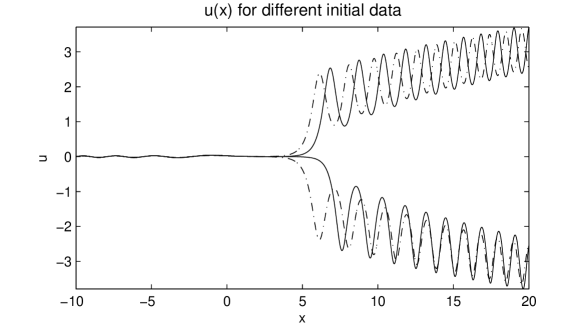
Figure 1: Dependance of $u(x)$ on the initial conditions

In figure 1, the solutions for $u_{x}(0)=-0.018$ and $u_{x}(0)=-0.017$, plotted discontinuously, tend respectively to $-\infty$ and $\infty$, and the solutions for $u_{x}(0)=-0.0175$ and $u_{x}(0)=-0.0174$, plotted continuously, tend respectively to $-\infty$ and $\infty$, although we observe that for these last two values, the explosion happens a bit later.

If we go farther with the process, between $u_{x}(0)=-0.0175$ and $u_{x}(0)=-0.0174$ there exists a unique $u_{x}(0)$ such that $\lim_{x\to\infty}u(x)=0$. That value, obtained with a bisection technique, is approximately $u_{x}(0)=-0.0174881944\ldots$ In figure 1, for scale reasons, we cannot distinguish clearly the oscillations in the real negative axis; in figure 2, having used the limit value for $u_{x}(0)$, those oscillations are displayed.

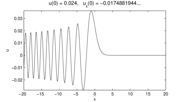
Figure 2: $u(x)$, with $\displaystyle{\lim_{x\to\infty}}u(x)=0$.

Because of the sensitivity with respect to initial data, we can calculate numerically only as many decimals of the correct $u_{x}(0)$ as the machine precision allows us, which implies that we are only delaying the explosion time for $u(x)$. We can say in an equivalent way that the solutions that make

$$\lim_{x\to\infty}u(x)=0$$ (21)

are highly unstable. Nonetheless, for our purposes, it is enough to consider $u(x)\equiv 0$ for a big enough $x$, because $u(x)\to 0$ exponentially as $x\to\infty$. Hence, since $|\int_{-\infty}^{0}u(x)dx|<\infty$, due to the fact that the oscillations in $x<0$ cancel one another, condition (21) is equivalent to $|\int_{-\infty}^{+\infty}u(x)dx|<\infty$.

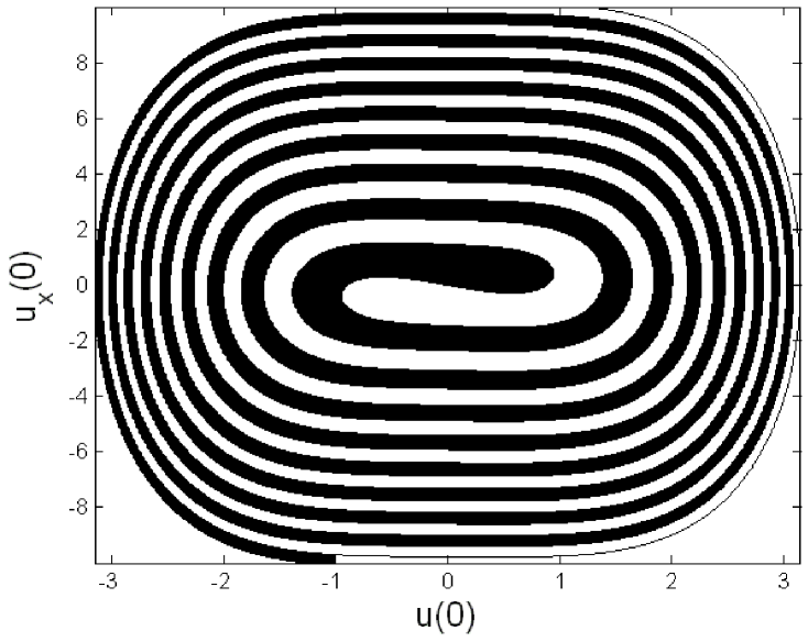
Figure 3: Pairs $(u(0),u_{x}(0))$, with $\displaystyle{\lim_{x\to\infty}}u(x)=+\infty$ (black) and $\displaystyle{\lim_{x\to\infty}}u(x)=-\infty$ (white)

In figure 3, the points belonging to the region in black, when taken as initial data $(u(0),u_{x}(0))$ of (19), give us solutions for (19) such that $u(x)\to+\infty$, as $x\to\infty$; for the points of the region in white, we have $u(x)\to-\infty$ instead. The boundary (figure 4) between both regions are the admissible pairs $(u(0),u_{x}(0))$ whose corresponding solutions satisfy (21). That boundary is a connected unbounded one-dimensional curve that divides the plane in two antisymmetrical halves. Each of the points of that curve determines one single self-similar $k(s,t)$, one single self-similar $\theta(s,t)$ and one single self-similar $z(s,t)$, which are solutions of (7), (18) and (6), respectively. Therefore, we have one-parameter families of solutions for (7), (18) and (6) that develop a singularity at finite time.

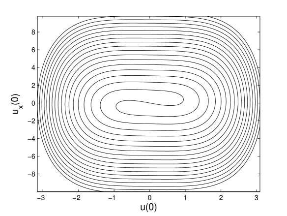
Figure 4: Admissible pairs. The points of this curve, when taken as initial data of (20), make $\displaystyle{\lim_{x\to\infty}}u(x)=0$.

3 A numerical method for the evolution of (6)

The $k(s,t)$, $\theta(s,t)$ and $z(s,t)$ we are considering are characterized by

$$k(-\infty,t) =0, k(+\infty,t) =0,$$

$$\theta(-\infty,t) =\theta^{-}, \theta(+\infty,t) =\theta^{+},$$

$$\lim_{s\to-\infty}|z(s,t) -se^{i\theta^{-}}|=0, \lim_{s\to+\infty}|z(s,t) -se^{i\theta^{-}}|=0.$$

Taking $\theta(s,t)$ as the evolution variable, we can preserver naturally $\int_{-\infty}^{+\infty}k(s,t)ds$ and $|z_{s}(s,t)|=1$. The PDE for $\theta$ with boundary conditions is

$$\begin{cases}\theta_{t}(s,t)=-\theta_{sss}(s,t)-\dfrac{1}{2}(\theta_{s})^{3}(s,t),\qquad s\in\mathbb{R},\\ \theta(-\infty,t)=\theta^{-},\\ \theta(+\infty,t)=\theta^{+}.\end{cases}$$ (22)

Due to the difficulty of considering the whole $\mathbb{R}$, we will restrict ourselves to $s\in[s_{a},s_{b}]$, with $s_{a}\ll-1$ and $s_{b}\gg 1$

$$\begin{cases}\theta_{t}(s,t)=-\theta_{sss}(s,t)-\dfrac{1}{2}(\theta_{s})^{3}(s,t),\qquad s\in[s_{a},s_{b}],\\ \theta(s_{a},t)=\theta^{-},\\ \theta(s_{b},t)=\theta^{+}.\end{cases}$$ (23)

$\theta(s,t)$ is not periodic in $[s_{a},s_{b}]$, so we define

$$\tilde{\theta}(s,t)=\theta(s,t)-{s-s_{a}\over L}(\theta^{+}-\theta^{-})-\theta^{-},\qquad L=s_{b}-s_{a},$$ (24)

which is periodic and regular for all $t>0$. (23) gets transformed into

$$\begin{cases}\tilde{\theta}_{t}(s,t)=-\tilde{\theta}_{sss}(s,t)-\dfrac{1}{2}\left(\tilde{\theta}_{s}(s,t)+\dfrac{\theta^{+}-\theta^{-}}{L}\right)^{3},\qquad s\in[s_{a},s_{b}],\\ \tilde{\theta}(s_{a},t)=\tilde{\theta}(s_{b},t)=0.\end{cases}$$ (25)

We will calculate the numerical evolution of $\tilde{\theta}$ at $N+1$ equidistant points $\{s_{j}\}$ in $[s_{a},s_{b}]$. Denoting with some abuse of notation $\hat{\theta}(\xi,t)\equiv(\tilde{\theta}(\xi,t))^{\wedge}$, we represent

$$\tilde{\theta}(s_{j},t)=\sum_{\xi=-N/2}^{N/2-1}\hat{\theta}(\xi,t)\exp\left[{2\pi i\xi\over L}(s_{j}-s_{a})\right],$$ (26)

where $L=s_{b}-s_{a}$, $\Delta s=\frac{L}{N}$ and $s_{j}=s_{a}+j\Delta s$. Therefore, (25) is transformed into

$$\hat{\theta}_{t}(\xi,t)=-\left(\dfrac{2\pi i\xi}{L}\right)^{3}\hat{\theta}(\xi,t)-\left[\dfrac{1}{2}\left(\tilde{\theta}_{s}(s,t)+\dfrac{\theta^{+}-\theta^{-}}{L}\right)^{3}\right]^{\bigwedge}(\xi,t),$$ (27)

with $\xi=-\frac{N}{2},\cdots,\frac{N}{2}-1$. Since we are working with the frequency, the third derivative is transformed into a multiplier that can be absorbed by means of an integrating factor

$$\left\{\hat{\theta}(\xi,t)\exp\left[t\left(\dfrac{2\pi i\xi}{L}\right)^{3}\right]\right\}_{t}\!\!\!=-\exp\left[t\left(\dfrac{2\pi i\xi}{L}\right)^{3}\right]\!\!\!\left[\dfrac{1}{2}\left(\tilde{\theta}_{s}(s,t)+\dfrac{\theta^{+}-\theta^{-}}{L}\right)^{3}\right]^{\bigwedge}\!\!\!(\xi,t).$$

The advantage of using an integrating factor is twofold: it allows to integrate exactly the linear part of (23), increasing the accuracy of the numerical results, and it relaxes considerably the time-step restrictions.

We apply the fourth-order Runge-Kutta in time with integrating factor as described in [18]. Denoting

$$\tilde{\Theta}^{0}(s) =\tilde{\theta}(s,t^{0}), \hat{\Theta}^{0}(\xi) =\hat{\theta}(\xi,t^{0}),$$

$$\tilde{\Theta}^{n}(s) \approx\tilde{\theta}^{n}(s)\equiv\tilde{\theta}(s,t^{n}), \hat{\Theta}^{n}(\xi) \approx\hat{\theta}^{n}(\xi)\equiv\hat{\theta}(\xi,t^{n}),\qquad t^{n}=t^{0}+n\Delta t,$$

we have

$$\hat{A}(\xi) =-\dfrac{1}{2}\left\{\left(\left[\left(\dfrac{2\pi i\xi}{L}\right)\hat{\Theta}^{n}(\xi)\right]^{\bigvee}+\dfrac{\theta^{+}-\theta^{-}}{L}\right)^{3}\right\}^{\bigwedge}(\xi),$$

$$\hat{\Theta}^{(A)}(\xi) =\exp\left[-\dfrac{\Delta t}{2}\left(\dfrac{2\pi i\xi}{L}\right)^{3}\right]\left(\hat{\Theta}^{n}(\xi)+\dfrac{\Delta t}{2}\hat{A}(\xi)\right),$$

$$\hat{B}(\xi) =-\dfrac{1}{2}\left\{\left(\left[\left(\dfrac{2\pi i\xi}{L}\right)\hat{\Theta}^{(A)}(\xi)\right]^{\bigvee}+\dfrac{\theta^{+}-\theta^{-}}{L}\right)^{3}\right\}^{\bigwedge}(\xi),$$

$$\hat{\Theta}^{(B)}(\xi) =\exp\left[-\dfrac{\Delta t}{2}\left(\dfrac{2\pi i\xi}{L}\right)^{3}\right]\hat{\Theta}^{n}(\xi)+\dfrac{\Delta t}{2}\hat{B}(\xi),$$

$$\hat{C}(\xi) =-\dfrac{1}{2}\left\{\left(\left[\left(\dfrac{2\pi i\xi}{L}\right)\hat{\Theta}^{(B)}(\xi)\right]^{\bigvee}+\dfrac{\theta^{+}-\theta^{-}}{L}\right)^{3}\right\}^{\bigwedge}(\xi),$$

$$\hat{\Theta}^{(C)}(\xi) =\exp\left[-\Delta t\left(\dfrac{2\pi i\xi}{L}\right)^{3}\right]\hat{\Theta}^{n}(\xi)+\Delta t\exp\left[-\dfrac{\Delta t}{2}\left(\dfrac{2\pi i\xi}{L}\right)^{3}\right]\hat{C}(\xi),$$

$$\hat{D}(\xi) =-\dfrac{1}{2}\left\{\left(\left[\left(\dfrac{2\pi i\xi}{L}\right)\hat{\Theta}^{(C)}(\xi)\right]^{\bigvee}+\dfrac{\theta^{+}-\theta^{-}}{L}\right)^{3}\right\}^{\bigwedge}(\xi),$$

$$\hat{\Theta}^{n+1}(\xi) =\exp\left[-\Delta t\left(\dfrac{2\pi i\xi}{L}\right)^{3}\right]\hat{\Theta}^{n}(\xi)+\dfrac{\Delta t}{6}\Bigg{\{}\exp\left[-\Delta t\left(\dfrac{2\pi i\xi}{L}\right)^{3}\right]\hat{A}(\xi)$$

$$+2\exp\left[-\dfrac{\Delta t}{2}\left(\dfrac{2\pi i\xi}{L}\right)^{3}\right]\left[\hat{B}(\xi)+\hat{C}(\xi)\right]+\hat{D}(\xi)\Bigg{\}},$$

$$t^{n+1} =t^{n}+\Delta t.$$

The symbols $\wedge$ and $\vee$ denote respectively the direct and inverse fast Fourier transforms (FFT) [9].

Finally, we force in every time step

$$\begin{cases}\tilde{\Theta}^{n+1}=(\hat{\Theta}^{n+1})^{\vee}\equiv\Re((\hat{\Theta}^{n+1})^{\vee})\\ \tilde{\Theta}^{n+1}(s_{0})=\tilde{\Theta}^{n+1}(s_{N})\equiv 0.\end{cases}$$ (28)

Rounding $\tilde{\Theta}^{n+1}$ to zero at the boundary points $s_{a}=s_{0}$ and $s_{b}=s_{N}$ avoids the accumulation of little errors of order $\mathcal{O}(10^{-9})$.

3.1 Computation of $\theta(s,1)$

Bearing in mind (10), at $t=1$, $\theta(s,1)$ is given by

$$\theta(s,1)-\theta(0,1)=\int_{0}^{s}k(s^{\prime},1)ds^{\prime}={2\over 3^{1/3}}\int_{0}^{s}u\left({s^{\prime}\over 3^{1/3}}\right)ds^{\prime}=2\gamma\left({s\over 3^{1/3}}\right),$$ (29)

where

$$\gamma(x)=\int_{0}^{x}u(x^{\prime})dx^{\prime};$$ (30)

hence, $\gamma_{x}=u$ and (20) can be generalized to

$$\begin{cases}\gamma_{x}=u,\\ u_{x}=v,\\ v_{x}=xu-2u^{3},\end{cases}$$ (31)

with initial data $u(0)$, $u_{x}(0)=v(0)$ and $\gamma(0)=0$. $(u(0),v(0))$ must be an admissible initial pair for (20), i.e., such that the corresponding $u(x)$ satisfies $\lim_{x\to\infty}u(x)=0$.

From now on, we will choose $u(0)=0.72$, $v(0)=1.1601860809647328$. In figure 5, we have integrated (31) in $x\in[-80,20]$, with $|\Delta x|=10^{-5}$. For $x\geq 9.204$, we have taken $k(x)\equiv 0$, because $|u(x)|<10^{-12}$. We obtain $\theta(s,1)$ from (29); hence, $s=3^{1/3}x$ and $s\in[\tilde{s}_{a},\tilde{s}_{b}]=[-115.38,28.84]$. Since we have one degree of freedom, we fix $\theta^{+}=\theta(\tilde{s}_{b},1)\equiv 0$.

As we observe in the lower part of figure 5, $\theta(s,1)$ tends to $\theta^{-}$ extremely slowly as $s\to-\infty$. Nevertheless, we can determine $\lim_{s\to-\infty}\theta(s,1)$ with high accuracy, as the mean value of the first maximum and the first minimum of $\theta(s,1)$, for $s>\tilde{s}_{a}$. In our example, the first maximum takes place at $s=-115.31$, being $\theta(-115.31,1)=-2.8403$; the first minimum takes place at $s=-114.80$, being $\theta(-114.79,1)=-3.0191$. Thus,

$$\lim_{s\to-\infty}\theta(s,1)=\theta^{-}\approx-2.9297\Rightarrow\int_{-\infty}^{+\infty}k(s^{\prime},1)ds^{\prime}=\theta^{+}-\theta^{-}\approx 2.9294,$$

quantity plotted in the lower part of figure 5 with a thinner stroke. In section 4, we will approximate the value of $\int_{-\infty}^{+\infty}k(s^{\prime},1)ds^{\prime}$ as a function of the admissible pairs $(u(0),u^{\prime}(0))$.

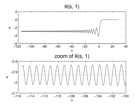
Figure 5: $\theta(s,1)$. In the zoomed image, we have plotted with a thinner stroke the mean between the first maximum and the first minimum of $\theta(s,1)$, for $s>s_{a}$, which gives a good estimate of $\theta^{-}$.

The $\theta(s,1)$ obtained after integrating (31) is not directly suitable as an initial datum of (23), because $\theta(\tilde{s}_{a},1)\not=\theta^{-}$ and (eq. 24)

$$\tilde{\theta}(s,1)=\theta(s,1)-{s-\tilde{s}_{a}\over L}(\theta^{+}-\theta^{-})-\theta^{-},\qquad L=\tilde{s}_{b}-\tilde{s}_{a},$$ (32)

is not periodic in $[\tilde{s}_{a},\tilde{s}_{b}]$. Hence, we have to modify $\theta(s,1)$ as follows:

• We chose $N_{1}\in\mathbb{N}$ and divide $[\tilde{s}_{a},\tilde{s}_{b}]$ into $N_{1}+1$ equidistant points $\{s_{j}\}$, in such a way that $0\in\{s_{j}\}$:

  $$s_{j}=\tilde{s}_{a}+j\Delta s,\quad\Delta s=\dfrac{\tilde{s}_{b}-\tilde{s}_{a}}{N_{1}},\qquad j=0,\ldots,N_{1}.$$

  We have taken $N_{1}=2000$; hence $\Delta s\approx 0.07211$ and $s_{1601}=0$.

• We find the $s_{j}$ with the lowest index, such that $s_{j}>s_{min}$, where $s_{min}$ is the first minimum point of $\theta(s,1)$ in $(s_{a},\infty)$, and $s_{j}$ satisfies that $\theta(s_{j},1)>\theta^{-}$ and $k(s_{j},1)=\theta_{s}(s_{j},1)>0$. We name it $s_{joint}$. Here, $s_{joint}=s_{13}\approx-114.51$, $\theta(s_{joint},1)\approx-2.9150$ and $k(s_{joint},1)\approx 0.5479$.

• We redefine $\theta(s,1)$, appending at $s=s_{joint}$ a smooth function that has a first order contact with $\theta(s,1)$ and tends exponentially to $\theta^{-}$ for $s<\tilde{s}_{a}$. The final expression for $\theta(s,1)$ is

  $$\theta(s,1)=\begin{cases}\theta(s,1),&s>s_{joint},\\ \theta^{-}+[\theta(s_{joint},1)-\theta^{-}]\exp\left[\dfrac{k(s_{joint},1)(s-s_{joint})}{[\theta(s_{joint},1)-\theta^{-}]}\right],&s\leq s_{joint},\end{cases}$$

  where, with some notational abuse, $\theta(s,1)$ stands for the original and the corrected functions.

• We evaluate the new $\theta(s,1)$ at the former $N_{1}+1$ points $\{s_{j}\}$, as well as in some new equidistant points $\{s_{j}\}$ outside $[\tilde{s}_{a},\tilde{s}_{b}]$. It is important that the final number of $\{s_{j}\}$ is $N+1\equiv 2^{n}+1$, for some $n\in\mathbb{N}$, in order to apply FFT efficiently. In the new set $\{s_{j}\}_{0}^{N}$, we define $s_{a}=s_{0}$, $s_{b}=s_{N}$.

The new function $\theta(s,1)$ satisfies $\theta(s_{a})=\theta^{-}$, $\theta(s_{b})=\theta^{+}$ and makes (24) periodic. We improve its regularity by applying a smooth spectral filter to (24)

$$\hat{\theta}(\xi,1)=\hat{\theta}(\xi,1)\exp\left[-10\left({2.5|\xi|\over N}\right)^{25}\right],$$ (33)

where $\hat{\theta}(\xi,1)\equiv(\tilde{\theta}(\xi,1))^{\wedge}$.

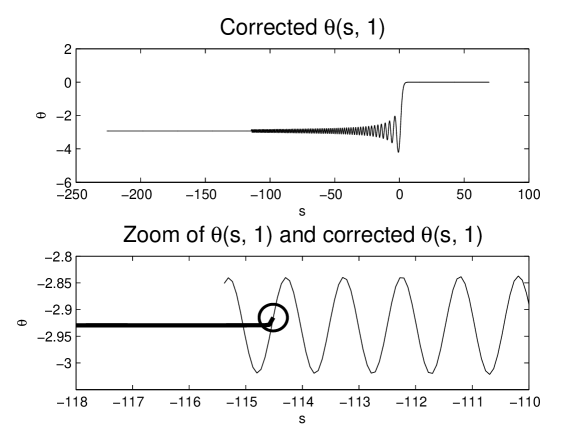
Figure 6: In the upper part, the final corrected $\theta(s,1)$ is plotted. In the lower part, both the original and the corrected $\theta(s,1)$ are plotted and zoomed near the joint (marked with a circle); the corrected $\theta(s,1)$ appears with a thicker stroke.

In figure 6, we have taken $N=4096$. In the upper part, we have plotted the final corrected $\theta(s,1)$, with $s\in[-226.14,69.23]$. We observe two long constant segments at the extremes of $\theta(s,1)$, because of the rather large choice of $N$; this is convenient to avoid periodicity phenomena, since the exact $\theta(s,1)$ is not periodic. In the lower zoomed part, we have plotted both the original and the corrected $\theta(s,1)$, highlighting the point $s=s_{joint}$ with a circle.

In its new form, it is immediate to obtain $\theta_{s}(s,t)$ from $\theta(s,t)$, through spectral derivation. Using again representation (24), we get

$$\theta_{s}(s,t)=\left[\theta(s,t)-{s-s_{a}\over L}(\theta^{+}-\theta^{-})-\theta^{-}\right]_{s}+\dfrac{\theta^{+}-\theta^{-}}{L},\qquad L=s_{b}-s_{a}.$$ (34)

Although the process to obtain $\theta(s,1)$ may look rather artificial, if we calculate $\theta_{s}(s,1)$ through (34) and compare it with the $k(s,1)$ obtained from integration of (31) and (10), we get the following error table:

$$\max_{s\in[-113.3,\infty)}|\theta_{s}(s,1)-k(s,1)|<10^{-3},$$

$$\max_{s\in[-110.6,\infty)}|\theta_{s}(s,1)-k(s,1)|<10^{-6},$$

$$\max_{s\in[-108.6,\infty)}|\theta_{s}(s,1)-k(s,1)|<10^{-8}.$$

Thus, $k(s,1)$ is recovered from the corrected $\theta(s,1)$ with high accuracy, except near the joint, $s_{joint}=-114.51$. This is graphically illustrated in figure 7; observe that the support of $\theta_{s}(s,1)$ is now finite.

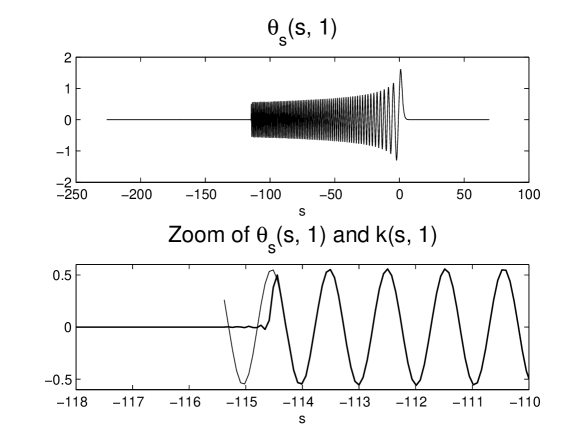
Figure 7: In the upper part, the derivative of the final corrected $\theta(s,1)$ is plotted; observe that its support is finite. In the lower part, the derivative of the corrected $\theta(s,1)$, plotted with a thicker stroke, is compared with the original $k(s,1)$.

$z(s,t)$ can also be immediately recovered from $\theta(s,t)$, except for a rigid movement, because $z_{s}(s,t)=\exp(i\theta(s,t))$. To fully determine $z(s,t)$, it is not complicate to see that

$$z(0,t)=-2(3t)^{1/3}\left[iu^{\prime}(0)+u^{2}(0)\right]z_{s}(0,t),$$ (35)

where $z_{s}(0,t)$ is a time-independent constant with unit modulus.

3.2 Numerical experiments

The aim of the method we have developed is to try to describe numerically the formation of the singularity in the self-similar solutions of equation (6) satisfying (10). This corner-shaped singularity happens at finite, time; indeed, at $t=0$, we have

$$z(s,0)=\begin{cases}z_{0}+se^{i\theta^{+}},&s\geq 0,\\ z_{0}+se^{i\theta^{-}},&s\leq 0.\end{cases}$$ (36)

Equivalently, when $t\to 0$, the curvature tends to a Dirac delta function

$$k(s,0)=a\delta(s),\qquad a=\int_{-\infty}^{+\infty}u(x)dx.$$ (37)

This happens because these self-similar solutions have infinite energy

$$\int_{-\infty}^{+\infty}k^{2}(s,t)ds=\infty,\qquad\forall t,$$

and it tends to concentrate at $s=0$ as $t\to 0$.

In our numerical experiments, we are not considering the whole $\mathbb{R}$, but $s\in[s_{a},s_{b}]$. At $s=s_{a}$ and $s=s_{b}$, we fix the tangent vector of $z$, i.e., $\theta(s_{a},t)=\theta^{-}$, $\theta(s_{b},t)=\theta^{+}$, for all $t$. As we observe in the upper part of figure 7, the support of the initial $k(s,1)$ of our numerical experiments is finite; hence, our numerical solutions have finite energy at $t=1$:

$$\int_{-\infty}^{+\infty}k^{2}(s,1)ds=\int_{s_{a}}^{s_{b}}k^{2}(s,1)ds<\infty.$$

We have executed the method with the initial $\theta(s,1)$ plotted in figure 6, i.e.,

$$\begin{cases}u(0)=0.72,\qquad u^{\prime}(0)=1.1601860809647328,\\ u(x)\mbox{ integrated when $x$}\in[-80,9.203],\\ s\in[-226.14,69.23],\qquad N=4096,\qquad\Delta s=0.07211.\end{cases}$$ (38)

In order to measure the quality of our results, we analyze two quantities: The evolution of the energy at $s\in[s_{a},s_{b}]$

$$\int_{s_{a}}^{s_{b}}k^{2}(s,t)ds,\qquad t\in[0,1],$$ (39)

and the curvature at the origin $s=0$, $k(0,t)$. From (10),

$$k(0,t)={2\over(3t)^{1/3}}u(0).$$ (40)

When considering the non-truncated problem with $s\in\mathbb{R}$, since all the infinite energy tends to concentrate

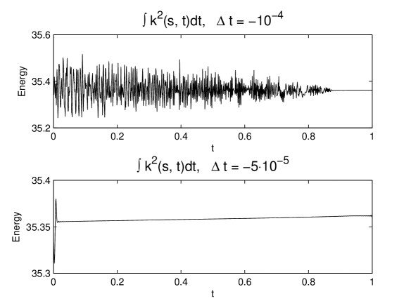
Figure 8: Numerical evolution of the energy in $s\in[s_{a},s_{b}]$, with initial data from (38). Unlike in the non-truncated case with $s\in\mathbb{R}$, the energy in the interval $s\in[s_{a},s_{b}]$ keeps approximately constant .

at $s=0$, the amount of energy (39) in $s\in[s_{a},s_{b}]$ grows up as we approach $t=0$, tending to infinity. On the contrary, in our numerical experiments, we have observed that the energy in the interval $s\in[s_{a},s_{b}]$ keeps approximately constant after having fixed $\theta(s_{a},t)=\theta^{-}$ and $\theta(s_{b},t)=\theta^{+}$; hence, we are preventing the energy outside the interval $s\in[s_{a},s_{b}]$ from entering.

In figure 8, we have plotted the energy (39) in $s\in[s_{a},s_{b}]$ for $\Delta t=-10^{-4}$ and $\Delta t=-5\cdot 10^{-5}$; remark that the energy conservation improves by diminishing $|\Delta t|$.

On the other hand, the accuracy of $k(0,t)$ is rather poor for small $t$ (see figure 9).

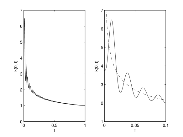
Figure 9: Numerical curvature at $s=0$, with initial data from (38) and $\Delta t=-5\cdot 10^{-5}$; the right-hand side figure is a magnification of the left-hand figure; the exact value (40) is plotted with a dotted stroke.

Numerical experiments show that the way to recover the curvature $k(0,t)$ with bigger accuracy near $t=0$ is not to diminish $|\Delta t|$ or $\Delta s$, but rather to introduce more energy to the system, i.e., to lengthen the support of the initial datum $k(s,1)$. To illustrate it, we have executed the method also with the following initial data:

$$\begin{cases}u(0)=0.72,\qquad u^{\prime}(0)=1.1601860809647328,\\ u(x)\mbox{ integrated when $x$ in }[-400,9.203],\\ s\in[-872.27,309.22],\qquad N=16384,\qquad\Delta s=0.07211\end{cases}$$ (41)

and

$$\begin{cases}u(0)=0.72,\qquad u^{\prime}(0)=1.1601860809647328,\\ u(x)\mbox{ integrated when $x$ in }[-800,9.203],\\ s\in[-1744.62,618.36],\qquad N=32768,\qquad\Delta s=0.07211.\end{cases}$$ (42)

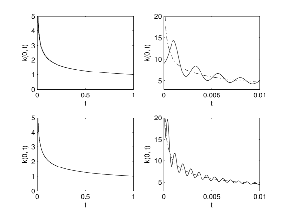
Figure 10: Curvature in $s=0$. The upper part graphics correspond to the experiment with data (41); the lower part graphics correspond to the experiment with data (42). The right-hand side graphics show $t\in[0,0.01]$, i.e., time values close to the singularity; the exact value (40) is plotted with dotted line.

Thus, we have made the initial support of $k(s,1)$ approximately five and ten times as big respectively, but with the same $\Delta s$ as in the previous experiment.

As we see in figure 10, we have been able to recover $k(0,t)$ until much smaller $t$. Remark that the results are better in the case where the support of $k(s,1)$ is bigger (lower right-hand side box). On the other hand, the observations about the energy are valid again (see figure 11).

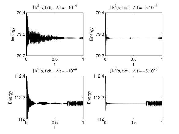
Figure 11: Numerical evolution of the energy. The upper part graphics correspond to the experiment with data (41). the lower part graphics correspond to the experiment with data (42).

In figure 12, we show the evolution of $k(s,t)$ in function of space and time, for the simulation with initial data (41). Clearly, the support of $k(s,t)$ tends to concentrate into $s=0$ with linear velocity, as $t\to 0$.

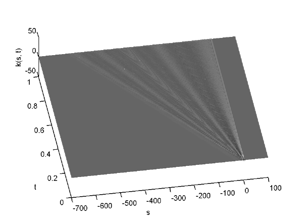
Figure 12: Numerical evolution of $k(s,t)$. The support of $k(s,t)$ tends to concentrate into $s=0$ with lineal velocity, as $t\to 0$.

Once we have obtained $\theta(s,t)$, it is immediate to recover $z(s,t)$, from $\theta(s,t)$, making $z_{s}(s,t)=\exp(i\theta(s,t))$, except for a rigid movement determined by (35). Nevertheless, from a numerical point of view, it is better for small times to fix $z(s_{b},t)\equiv z(s_{b},0)$. In figure 13, we have superimposed the graphs of $z(s,t)$ in a neighborhood of $s=0$, with initial data (41), at times $t=1$, $t=0.5$, $t=0.1$, $t=0.01$ and $t=0.001$, having fixed $z_{s}(0,t)=1$. We can clearly appreciate the self-similar character of the solutions.

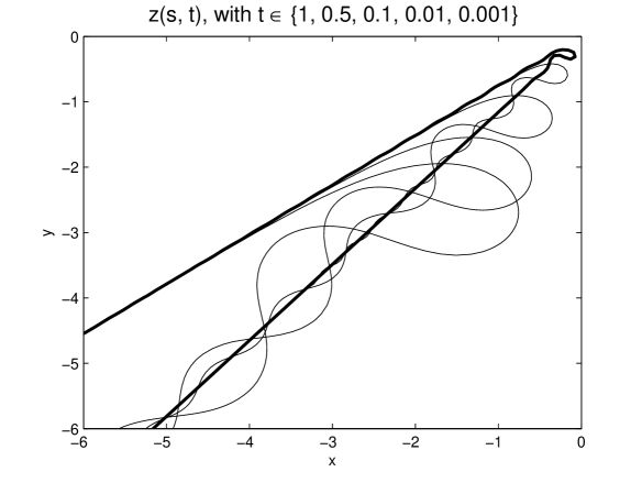
Figure 13: Numerical evolution of $z(s,t)$ for different times, with initial data (41). The self-similarity is patent. The thick dark curve corresponds to $t=0.001$.

In figure 14, we have plotted with a thicker stroke the admissible pairs for which $z(s,t)$ has no self-intersections, highlighting with a circle the pair that we have used in our experiments. Figure 13 and figure 14 explain why we have chosen $(u(0),u^{\prime}(0))=(0.72,1.1601860809647328)$. Indeed, we have taken an admissible pair for which $z(s,t)$ has no self-intersections, but such that it is near the situation when self-intersections happen; because of that, $\int k(s,t)ds>2.92$, i.e., a value near $\pi$. Theorems 1 and 2 only guarantee the formation of the singularity for small values of $\int_{-\infty}^{+\infty}k(s^{\prime},t)ds^{\prime}=\theta^{+}-\theta^{-}$, but the previous results and figure 14 give evidence that they also true for any value of $\theta^{+}-\theta^{-}\in(-\pi+\varepsilon,\pi-\varepsilon)$, $0<\varepsilon\ll 1$ (cf. section 4). In any case, all admissible data on the dark, ’s’ shaped curve in figure 14 give self-similar corner solutions.

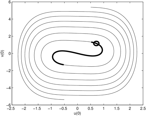
Figure 14: The thick dark curve shows the admissible pairs $(u(0),u_{x}(0))$, such that $z(s,t)$ has no self-intersections. The circle indicates the pair that we have considered.

Before finishing this section, let us underline four main conclusions:

• The finite energy in $[s_{a},s_{b}]$ keeps approximately constant after fixing the tangent vector of $z(s,t)$ at $s=s_{a}$ and $s=s_{b}$.

• The support of $k(s,t)$, and hence, the energy, tend to concentrate into $s=0$ with lineal velocity, as $t\to 0$.

• $k(0,t)$ is well recovered, even for small $t$. To recover $k(0,t)$ for smaller times, it is necessary to consider a bigger support of $k(s,1)$.

• Our numerical results generalize theorems 1 and 1, because they give evidence that the formation of the corner singularity happens for any value of $\theta^{+}-\theta^{-}\in(-\pi+\varepsilon,\pi-\varepsilon)$, $0<\varepsilon\ll 1$.

Hence, we are approximating a Dirac delta function (8), but we will never been able to create a singularity, because the energy is finite. In the non-truncated problem, with $s\in\mathbb{R}$, the energy is infinite for all $t$ and it tends to concentrate at $s=0$ as $t\to 0$, which causes the singularity (8).

Because of the parallelisms between the truncated and the non-truncated problem, we can say that our numerical solutions reproduce the non-truncated problem from a qualitative point of view, suggesting that we could approach the Dirac delta function as much as we want, by increasing the initial support of $k(s,1)$. It would be very interesting to prove analytically that we can recover the exact problem by making $s_{a}\to-\infty$, $s_{b}\to+\infty$.

4 $\int k(s^{\prime},t)dt$, in terms of $u(0)$ and $u_{x}(0)$

As seen in section 3.1, obtaining $\theta(s,1)$ for our experiments involves an estimate of $\int_{-\infty}^{+\infty}k(s^{\prime},1)ds^{\prime}$. This integrate is hence determined by one admissible pair of initial data $(u(0),u_{x}(0))$ of (eq. 19), i.e., one point of the curve in figure 4.

We have integrated (31) in $x\in[-80,20]$, $|\Delta x|=10^{-5}$, for a large set of admissible pairs $(u(0),u_{x}(0))$ taken as initial conditions. Following exactly the same steps as in 3.1, we have estimated $\int_{-\infty}^{+\infty}k(s^{\prime},1)ds^{\prime}$.

In figure 15, each admissible pair $(u(0),u_{x}(0))$ appears together with its corresponding estimate of $\int_{-\infty}^{+\infty}k(s^{\prime},1)ds^{\prime}$;

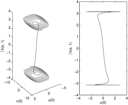
Figure 15: Integral of the curvature. The left-hand side shows the admissible pairs $(u(0),u_{x}(0))$, together with their corresponding integral $\int_{-\infty}^{+\infty}k(s^{\prime},1)ds^{\prime}$. The right-hand side is a side view of the left-hand side.

the curve we have plotted in this way is antisymmetric with respect to the origin.

For the set of admissible data considered, our numerical estimates satisfy

$$-\pi-5.6\cdot 10^{-4}<\int_{-\infty}^{+\infty}k(s^{\prime},1,u(0),u^{\prime}(0))ds^{\prime}<\pi+5.6\cdot 10^{-4}.$$ (43)

Hence, there is strong numerical evidence to accept that

$$\int_{-\infty}^{+\infty}u(x)dx\in\left(-\dfrac{\pi}{2},\dfrac{\pi}{2}\right)\Longleftrightarrow\int_{-\infty}^{+\infty}k(s^{\prime},t)ds^{\prime}\in(-\pi,\pi),\qquad\forall t.$$ (44)

For values of the integral in $[-3-\varepsilon,3+\varepsilon]$, $0<\varepsilon\ll 1$, it is evident from the right-hand side part, which represents the first and third components of the curve on the left-hand side, that there is only one corresponding initial condition for (19). The values of the integral seem to converge exponentially to $\pm\pi$. We are prone to think that there is one single initial condition for each value in $(-\pi,\pi)$, although if we have exponential convergence, it will be much more difficult to give numerical evidence for the values nearest to $\pm\pi$.

5 Using a simple closed $z(s,1)$ as initial data

Coming back to our second experiment, with initial data (41), and motivated by the vortex patch problem, it is interesting to see what happens if we add a big loop to $z(s,1)$, so that it becomes a simple closed curve without intersections. For that purpose, we have appended a smooth function to $\theta(s,1)$ at $s=s_{a}$, such that the new value for $\theta^{+}-\theta^{-}$ is $\theta^{+}-\theta^{-}=2\pi$. This function is a rescaling of

$$\Psi(s) =\int_{0}^{s}\psi(s^{\prime})ds^{\prime},\quad s\in[0,1],$$ (45)

with

$$\psi(s) =\begin{cases}0,&s\in[0,\alpha)\cup\{1\},\\ \exp\left[\dfrac{-\beta}{(x-\alpha)(1-x)}\right],&s\in(\alpha,1),\end{cases}$$ (46)

being both $\psi$ and $\Psi$ are regular in $[0,1]$.

In what follows, we have rotated $z$ in such a way that $z_{s}(s_{a})=1$.

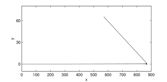
Figure 16: $z(s,1)$ corresponding to the initial data (41) before being closed

If we plot the $z$ corresponding to initial data (41), we observe in figure 16 that the lower asymptotic line of $z$ is much longer than the upper one. That is why we have defined $\psi(s)$ being $\psi(s)\equiv 0$ in a certain $[0,\alpha]$, in order to prolong the upper asymptotic line of $z$ before closing $z$ by means of a loop; the choice of $\alpha$ determines the additional length that we add to the upper asymptotic line, whereas the choice of $\beta$ determines the length of the loop. We have to adjust both parameters wisely, so that $z$ becomes smoothly closed.

Remembering that $\theta(s,1)$ was defined in such a way that $\theta(s_{b})=0$, the new expression for $\theta(s,1)$ looks like this:

$$\theta(s,1)=\begin{cases}\theta(s,1),&s\in[s_{a},s_{b}]\\ \dfrac{2\pi-\theta(s_{a},1)}{\Psi(1)}\Psi\left(\dfrac{s-s_{b}}{3(s_{b}-s_{a})}\right),&s\in[s_{b},s_{b}+3(s_{b}-s_{a})],\end{cases}$$ (47)

i.e., we have made four times as big the length of the new $[s_{a},s_{b}]$ and our new $s_{b}$ is $s_{b}=s_{b}+3(s_{b}-s_{a})$; the new amount of nodes $s_{j}$ is $4N+1=65537$, so that $\Delta s$ remains unchanged. Notice that, with some notational abuse, $\theta(s,1)$ refers to both the old and the prolonged functions and $s_{b}$ to the old and the new right extreme. The new $\theta$ satisfies $\theta(s_{b},1)-\theta(s_{a},1)=2\pi$. This is a necessary but not sufficient condition in order that $z$ may be closed. To determine $\alpha$ and $\beta$, we proceed as follows:

If $\alpha$ is fixed, by a bisection technique, we determine a $\beta$ such that $\Im(z(s_{b},1))=0$. Then, for some values of $\alpha$, $\Re(z(s_{b}),1)$ will be positive, while for some other values, it will be negative. For instance, for two choices of $\alpha$, $\alpha=0.1$ and $\alpha=0.2$, we have applied the bisection technique to find the corresponding $\beta$ in $[0.5,20]$. At the end of the process, $z(s_{b},1)$ is not exactly real, but its imaginary part is negligible

$$\alpha =0.1 \Rightarrow \begin{cases}\beta=5.492976875712412\\ z(s_{b},1)\approx 209+5i\cdot 10^{-12}\end{cases}$$

$$\alpha =0.2 \Rightarrow \begin{cases}\beta=2.824543846424351\\ z(s_{b},1)\approx-146-i\cdot 10^{-12}.\end{cases}$$

Now, we have to apply the bisection technique to $\alpha$. For example, for $\alpha=0.15$, we have $\beta=3.970063345682464$ and $z(s_{b},1)\approx 32-2i\cdot 10^{-12}$.

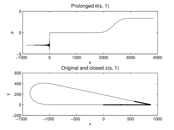
Figure 17: New $\theta(s,1)$ and $z(s,1)$

That means that the correct $\alpha\in[0.15,0.2]$. After several iterations, the double-bisection algorithm yields

$$\begin{cases}(\alpha,\beta)=(0.158902181218767,3.741222383167766)\\ z(s_{b},1)\approx(2+3i)\cdot 10^{-12}.\end{cases}$$ (48)

Since $s\in[-872.27,3853.69]$ and $z(s,1)$ is parameterized respect to the arc-length parameter, the length of the curve is $4725.96$. In figure 17, we can see the prolonged version of $\theta(s,1)$, as well as $z(s,1)$, with and without the loop. We have closed $z(s,1)$ almost in a perfect way, because $z(s_{b},1)-z(s_{a},1)=\mathcal{O}(10^{-12})$.

When $z$ is closed, $z_{s}(0,t)$ is obviously no longer constant and (35) does not hold any more; in fact, $z(s,t)$ will rotate, so we need to give the evolution of a point and its angle for all $t$, which is quite straightforward. We just have to integrate the following two ODE’s in $t$ for some $s_{0}$:

$$\theta_{t}(s_{0},t) =-\theta_{sss}(s_{0},t)-\dfrac{1}{2}\theta_{s}^{3}(s_{0},t),$$

$$z_{t}(s_{0},t) =-z_{sss}(s_{0},t)+\dfrac{3}{2}\bar{z}_{s}(s_{0},t)z_{ss}^{2}(s_{0},t).$$

The right-hand side of the first equation is known, so we can update $\theta(s_{0},t^{n})$. Then, bearing in mind that $z_{s}(s_{0},t^{n})=\exp(i\theta(s_{0},t^{n}))$, the right-hand side of the second equation is also known and we update $z(s_{0},t^{n})$.

In any case, since this paper aims at illustrating the energy concentration process, we will not rotate $z$, in order to compare the situations with and without the loop.

5.1 Numerical experiments

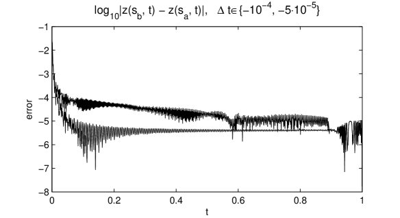
Figure 18: Error when closing $z(s,t)$. The error is smaller for $\Delta t=-5\cdot 10^{-5}$.

We have executed the method with the new $\theta(s,1)$. Remark that the evolution variable is $\theta$, not $z$, so the method does not guarantee a priori that $z(s_{a},t)=z(s_{b},t)$, for all $t$.

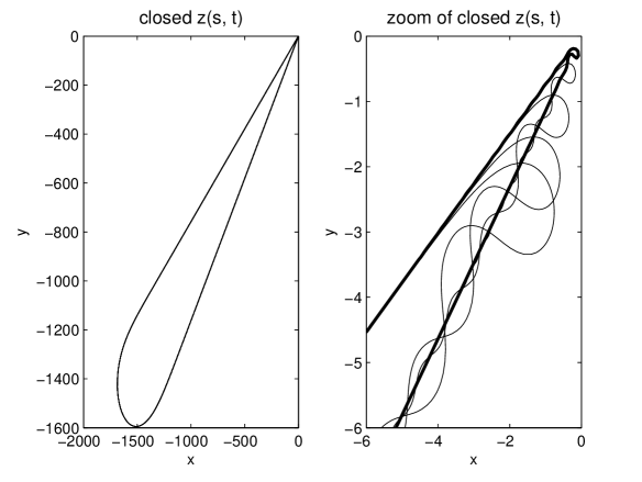
Figure 19: $z(s,t)$ and zoom of $z(s,t)$, for $t\in\{1,0.5,0.1,0.01,0.001\}$. The thick dark curve at the right-hand side corresponds to $t=0.001$.

Nevertheless, the curve keeps closed with great accuracy, as we can see in figure 18, where we have plotted the decimal logarithm of $|z(s_{b},t)-z(s_{a},t)|$, for $\Delta t$ small enough. Indeed, for $\Delta t=-5\cdot 10^{-5}$, $|z(s_{a},t)-z(s_{b},t)|<10^{-4}$ until very small times and, since the length of the curve is approximately $4726$, that means a relative error smaller than $10^{-7}$.

On the other hand, the loop does not have any visible influence on the formation of the corner-shaped singularity for $z(s,t)$. In figure 19, we have plotted $z(s,t)$, with $z_{s}(0,t)=1$, for $t=1$, $0.5$, $0.1$, $0.01$ and $0.001$. In the left-hand side part, all the plots seem to be a single one; nevertheless, after a potent zoom, the formation of the singularity at $s=0$ is clearly exhibited. In fact, the right-hand side of the figure is not ocularly distinguishable from figure 13.

From the left-hand side of figure 19, it is obvious that the enclosed area remains almost constant, for all $t$. We can check this by means of the well known formula:

$$\mbox{Area}=\dfrac{1}{2}\oint(xdy-ydy)=\dfrac{1}{2}\int_{s_{a}}^{s_{b}}[x(s)y^{\prime}(s)-x^{\prime}(s)y(s)]ds,\quad z=x+iy,$$ (49)

which is a direct application of Green’s theorem. Figure 20 shows that the enclosed area is preserved with great accuracy.

Figure 20: Preservation of the area enclosed by $z$

6 Conclusions

In this paper, we have consider a geometric planar flow (eq. 1) found by Goldstein and Petrich [11], while considering the evolution of a vortex patch. Perelman and Vega proved in [17] that it has a one-parameter family of solutions that develop corner-shaped singularities at finite time. We have studied those solutions from a numerical point of view, trying to reproduce the singularity formation.

The flow can be characterized by the equation of its curvature, $k$, which is the modified Korteweg-de Vries (7) equation. Nevertheless, we have found the angle $\theta=\int^{s}kds^{\prime}$ to be the most adequate evolution variable, because it allows to preserve naturally the arc-length parameter and the angle formed by the two asymptotic lines of $z$. Due to the difficulty of considering the whole $\mathbb{R}$, we have taken $s\in[s_{a},s_{b}]$. The main result is that, even after fixing $\theta(s_{a},t)=\theta^{-}$, $\theta(s_{b},t)=\theta^{+}$, i.e., after fixing the tangent vectors of $z$ at $s_{a}$ and $s_{b}$, we are still able to approximate the formation of the corner-shaped singularity. Indeed, the energy $\int_{s_{a}}^{s_{b}}k^{2}(s^{\prime},t)ds^{\prime}<\infty$ keeps approximately constant and it tends to concentrate at $s=0$; moreover, we recover with great accuracy $k(0,t)$, even for small $t$, tending $k$ to a Dirac delta function. The numerical results suggest that the accuracy of $k(0,t)$ could be improved arbitrarily by increasing the length of $[s_{a},s_{b}]$; it would be very interesting to prove analytically that we can recover the solution of the exact problem by making $s_{a}\to-\infty$ and $s_{b}\to\infty$.

The process of obtaining the initial $\theta$ involves an estimate of the conserved quantity $\int_{-\infty}^{+\infty}k(s^{\prime},t)ds^{\prime}$. We have given numerical evidence that $|\int_{-\infty}^{+\infty}k(s^{\prime},t)ds^{\prime}|<\pi$.

Motivated by the vortex patch problem, we have also considered a regular simple closed curve as initial datum, by appending a regular function to $\theta(s,1)$ in such a way that $z(s,1)$ is closed by a big loop. The method preserves the area enclosed by the curve with great accuracy and, more interestingly, the loop appears to have no influence on the energy concentration process; nevertheless, no singularities can be expected because the energy of our curves is finite [13, 4]. This is in agreement with the vortex patch theory, where it is known that no singularities may arise from smooth initial contours [5, 3]. In [17], Perelman and Vega considered instead infinite energy solutions of the mKdV equation, which causes the singularity to happen.

One of the shortcomings of our model is that the arc-length parameter is preserved for a simple closed curve and, hence, the total length of the curve remains constant. In the vortex patch problem, on the contrary, there are examples in which the length or curvature of the vortex patch boundary grow rapidly [1, 6]. Therefore, the mKdV equation should be complemented by another equation for the evolution of $s_{\alpha}$.

7 Acknowledgements

The author would want to express his gratitude to L. Vega and C. García-Cervera for very valuable advice concerning this paper.

References

[1]S. Alinhac, Remarques sur l’instabilité du problème des poches de
tourbillon, J. Funct. Anal, 98 (1991), pp. 361–379.
[2]G. K. Batchelor, An Introduction to Fluid Dynamics, Cambridge
University Press, Cambridge, 1967.
[3]A. L. Bertozzi and P. Constantin, Global regularity for vortex
patches, Commun. Math. Phys., 152 (1993), pp. 19–28.
[4]J. Bourgain, Fourier transform restriction phenomena for certain
lattice subsets and applications to nonlinear evolution equations. part ii:
The kdv-equation, Geom. Funct. Anal., 3 (1993), pp. 209–262.
[5]J. Y. Chemin, Persistency of geometric structures in bidimensional
incompressible fluids, Ann. Sci. Ecole Norm. Sup., 26 (1994), pp. 517–542.
[6]P. Constantin and E. S. Titi, On the evolution of nearly circular
vortex patches, Commun. Math. Phys., 119 (1988), pp. 177–198.
[7]G. S. Deem and N. J. Zabusky, Vortex waves: Stationary “v.
states”, interactions, recurrence and breaking, Phys. Rev. Lett., 40
(1978), pp. 859–862.
[8]D. G. Dritschel, The repeated filamentation of two-dimensional
vorticity interfaces, J. Fluid Mech., 194 (1988), pp. 511–547.
[9]M. Frigo and S. G. Johnson, The design and implementation of
FFTW3, Proceedings of the IEEE, 93 (2005), pp. 216–231.
special issue on ”Program Generation, Optimization, and Platform
Adaptation”.
[10]R. E. Goldstein and D. M. Petrich, The korteweg-de vries hierarchy
as dynamics of closed curves in the plane, Phys. Rev. Letters., 67 (1991),
pp. 3203–3206.
[11], Soliton’s, euler’s
equations, and vortex patch dynamics, Phys. Rev. Letters., 69 (1992),
pp. 555–558.
[12]H. Hasimoto, A soliton in a vortex filament, J. Fluid Mech., 51
(1972), pp. 477–485.
[13]C. E. Kenig, G. Ponce, and L. Vega, Well-posedness and scattering
results for the generalized korteweg-de vries equation via the contraction
principle, Comm. Pure Appl. Math., 46 (1993), pp. 527–620.
[14]G. L. Lamb, Jr, Solitons on moving space curves, J. Math Phys.,
18 (1977), pp. 1654–1661.
[15]A. J. Majda and A. L. Bertozzi, Vorticity And Incompressible Flow,
Cambridge Texts in Applied Mathematics, Cambridge University Press,
Cambridge, 2002.
[16]K. Nakayama, H. Segur, and M. Wadati, Integrability and the motion
of curves, Phys. Rev. Letters, 69 (1992), pp. 2603–2606.
[17]G. Perelman and L. Vega, Self-similar planar curves related to
modified korteweg-de vries equation, J. of Diff. Eqns, 235 (2007),
pp. 56–73.
[18]L. N. Trefethen, Spectral Methods in Matlab, SIAM, Philadelphia,
Pennsylvania, 2000.
[19]C. Wexler and A. T. Dorsey, Contour dynamics, waves, and solitons in
the quantum hall effect, Phys. Rev. B, 60 (1999), pp. 10971–10983.