Shock Speed, Cosmic Ray Pressure, and Gas Temperature in the Cygnus Loop

Abstract

Upper limits on the shock speeds in supernova remnants can be combined with post-shock temperatures to obtain upper limits on the ratio of cosmic ray to gas pressure ($P_{CR}/P_{G}$) behind the shocks. We constrain shock speeds from proper motions and distance estimates, and we derive temperatures from X-ray spectra. The shock waves are observed as faint H$\alpha$ filaments stretching around the Cygnus Loop supernova remnant in two epochs of the Palomar Observatory Sky Survey (POSS) separated by 39.1 years. We measured proper motions of 18 non-radiative filaments and derived shock velocity limits based on a limit to the Cygnus Loop distance of 576 $\pm$ 61 pc given by Blair et al. for a background star. The PSPC instrument on-board ROSAT observed the X-ray emission of the post-shock gas along the perimeter of the Cygnus Loop, and we measure post-shock electron temperature from spectral fits. Proper motions range from 2$\farcs$7 to 5$\farcs$4 over the POSS epochs and post-shock temperatures range from $kT\sim 100-200\rm~{}eV$. Our analysis suggests a cosmic ray to post-shock gas pressure consistent with zero, and in some positions $P_{CR}$ is formally smaller than zero. We conclude that the distance to the Cygnus Loop is close to the upper limit given by the distance to the background star and that either the electron temperatures are lower than those measured from ROSAT PSPC X-ray spectral fits or an additional heat input for the electrons, possibly due to thermal conduction, is required.

1. Introduction

Supernova explosions are responsible for showering the surrounding interstellar medium (ISM) with heavy elements, influencing the distribution and composition of gas in the host galaxy. A typical supernova releases $\sim$10⁵¹ ergs, sending a highly supersonic shock wave into its surroundings at speeds of up to 30,000 km s^-1 (Ghavamian et al. 2001). This expanding surge of energy heats and ionizes the neighboring gas out to hundreds of parsecs, initiating cloud collapse which leads to star formation and galactic evolution. Although a supernova is short-lived, the ejected remains propagate outward and interact with the ISM. These supernova remnants (SNRs) radiate over a large spectral range, transporting information about the blast wave morphology and local ISM.

The Cygnus Loop is a well-known SNR whose distance is less than 576 $\pm$ 61 pc based on the distance to a star whose spectrum shows absorption features from shocked gas in the remnant (Blair et al., 2008). From a global perspective, its structure is governed by interactions with the surrounding inhomogeneous ISM. Despite its apparent spherical symmetry, both optical and X-ray observations suggest that the Cygnus Loop does not follow the simplified Sedov-Taylor morphology of an adiabatic blast wave expanding into a homogeneous, low density medium. Instead, the blast wave deceleration is the result of encounters with dense, extended clouds distributed inhomogeneously in the pre-shocked gas (Levenson et al., 1997; Levenson et al., 1998).

We focus on the non-radiative H$\alpha$ shock filaments, primarily in the northeastern Cygnus Loop, several of which were previously observed by Hester et al. (1994), Blair et al. (1999, 2008), Ghavamian et al. (2001) and Raymond et al. (2003). In a non-radiative shock, the cooling timescale of the hot shocked gas is much greater than the age of the shock. As the shocked gas has not had sufficient time to cool, post-shock radiation does not affect the shock evolution (McKee & Hollenbach, 1980). Therefore, non-radiative shock filaments provide a laboratory for probing the conditions at the shock front before this information is lost by radiative or collisional processes. When a non-radiative shock encounters neutral gas, Balmer line emission is produced by the excitation of neutral hydrogen atoms prior to ionization. The resulting H$\alpha$ filaments trace the outer edge of the Cygnus Loop non-radiative blast wave as it expands through low density, partially neutral gas. These H$\alpha$ filaments are useful for proper motion measurements of shock fronts and investigations of shocked gas parameters.

SNR shock waves are believed to accelerate cosmic rays up to energies of 10¹⁵ eV and to be responsible for a large fraction of interstellar cosmic rays, implying an efficient process for particle acceleration. The theory of diffusive shock acceleration describes how charged particles (dominantly protons and electrons) passing back and forth across a shock front reach high energies, resulting in a power-law spectrum $\propto$ E^-2 for cosmic rays above $\sim$ 10⁹ GeV (Blandford & Eichler, 1987). This particle acceleration process requires a collisionless medium, as frequent collisions would return the velocity profile to Maxwellian.

The efficiency of energy conversion in SNR shocks into the acceleration of cosmic rays is highly dependent on shock structure and is a topic of active research. Theory indicates that the fraction of the energy dissipated in a shock going into cosmic rays is bistable, being either very small or $\sim$ 80% (Malkov et al. 2000). Recent calculations of the evolution of SNR shocks show that the efficiency starts off low and evolves gradually to somewhat smaller values than that predicted by steady shock models (Caprioli et al. 2008). Synchrotron emission in the radio and X-ray bands provides direct observation of particle acceleration in SNRs; however, the majority of the SNR energy going into particle acceleration is claimed by protons. Our current observational ability to detect $\gamma$-rays (and neutrinos) is limited, so we must settle for inferences of the total cosmic ray acceleration efficiency through indirect methods. Warren et al. (2005) inferred shock compression ratios greater than 4 from the distance between the blast wave and the contact discontinuity in Tycho’s SNR. Their results suggest that the cosmic ray to gas pressure ratio, $P_{CR}/P_{G}>1$, though projection effects might allow a smaller compression ratio (Cassam-Chenai et al. 2008). High cosmic ray acceleration efficiencies have also been inferred from the low electron temperature in 1E102-72.6 (Hughes et al. 2000) and from shock wave precursors to Balmer line filaments (Smith et al. 1994; Hester et al. 1994).

In this paper we find upper limits to $P_{CR}/P_{G}$ by combining measurements of post-shock electron temperature with the shock speed given by proper motions and distance upper limits. Our sample includes 18 non-radiative H$\alpha$ shock segments dominantly in the northeastern rim of the Cygnus Loop. This sample, although limited by the uncertainties in proper motion, temperature, and distance, provides constraints on $P_{CR}/P_{G}$. Several positions show apparently negative values of $P_{CR}$, and we discuss the uncertainties in temperature and distance and the possibility of additional electron heating that could account for that non-physical result.

2. Observations and Data Reduction

We observe regions in the northern, eastern, and western Cygnus Loop over optical and X-ray bands. The Palomar Observatory Sky Survery (POSS) obtained the optical data and the ROSAT Position Sensitive Proportional Counter (PSPC) obtained the X-ray data. We reduced two epochs of optical data for proper motion measurements. The X-ray data were obtained within two years of the more recent optical epoch. We matched WCS coordinates of all data to ensure consistency during optical and X-ray analysis.

2.1. POSS Optical Data Reduction

The POSS observed the Cygnus Loop over two epochs spanning 39.1 years. These photographic plates have been digitized by the Space Telescope Science Institute (STScI) and are publicly archived as the Digitized Sky Survey. We selected the filtered surveys whose transmission coefficient peaked near H$\alpha$ ($\lambda=6562.8~{}\mbox{\AA}$), corresponding to surveys POSS-I E (red) and POSS-II F (red), to ensure detection of H$\alpha$ shock filaments along the Cygnus Loop perimeter. We refer to the 1953 June 15 observations as POSS-I and the 1992 July 24 observations as POSS-II, with exposure times of 45.0 and 120 minutes, respectively. The pixel scales of the digitized POSS-I and POSS-II plates are 1$\farcs$7 and 1$\farcs$0, respectively.

We analyzed proper motions of 18 H$\alpha$ shock filaments which define the perimeter of the Cygnus Loop. We used IDL and SAOImage DS9 for subsequent image analysis. From each POSS epoch, we hand selected a sub-image containing the filament of interest surrounded by reference background and foreground stars based on a common WCS (J2000) position. POSS-I and POSS-II pixel scales were resampled to 0$\farcs$1 using bilinear interpolation between grid points. Each set of sub-images was rotated appropriately to account for precession effects during the time between observations. An additional rotation was incorporated to align the shock along the image axis for the proper motion analysis. Two-dimensional cross-correlation methods determined an optimal fine-tuned pixel shift to overlap the POSS-I and POSS-II sub-images. In the resulting images the background stars are stationary, leaving the propagating shock for analysis. All image manipulation was made relative to the POSS-I plate in an attempt to maintain the original integrity of the data.

2.2. ROSAT PSPC X-Ray Data Reduction

The Cygnus Loop X-ray data we analyzed were obtained with the PSPC detector on-board the ROSAT observatory. The observation timeline spans from 1992 Nov 04 to 1994 June 03 with 3 separate pointings targeting 3 locations. Table 1 lists the ROSAT PSPC observations relevant to our X-ray post-shock analysis of the Cygnus Loop. All observed data sets are publicly archived through the HEASARC.

To prepare the ROSAT PSPC data for analysis, spectral regions were extracted from the PSPC events files requiring a minimum of 1,200 counts within each region. Source and background spectra were extracted and truncated to Pulse Invarient (PI) channels 0-255 using xselect version 2.4. We filter PSPC spectra to accept good events and, since we will be using $\chi^{2}$ statistics, we require a minimum of 20 counts per bin using the FTOOL grppha. We extracted X-ray emitting regions extending from 25″ to 100″ behind each H$\alpha$ filament of interest. As discussed below, we avoided the region within 25″ where the gas is significantly out of ionization equilibrium. Background spectra were taken outside the outer shock front and scaled by the ratio of the areas of the extraction regions. PSPC response matrices were obtained from the legacy.gsfc.nasa.gov anonymous ftp archive and ancillary response files (ARFs) were generated using the FTOOL pcarf as outlined by Turner (1996). The resulting spectra were fit with XSPEC version 11.3.2 (Arnaud, 1996). The PSPC detector is calibrated over the 0.1-2 keV soft X-ray energy band (Prieto, 1996). All spectra were fit in the 0.1-1.1 keV band as more energetic photons were not typically detected. The X-ray errors presented in this paper are at the 90% confidence level obtained with the XSPEC error command unless otherwise indicated.

3. Analysis and Results

We surveyed 18 shock filaments, each of length 120″, spanning the eastern, northern, and western Cygnus Loop outer shell which is defined by its characteristic H$\alpha$ emission. For each filament, we measured proper motion by comparing two epochs of POSS red digitized plates and post-shock gas temperature from spectral fits to ROSAT PSPC X-ray data, assuming ionization equilibrium. Adopting the most recent distance upper limit to the Cygnus Loop of 576 $\pm$ 61 pc (Blair et al., 2008), we constrain the ratio of cosmic ray to gas pressure. We discuss our methodology, the uncertainties in proper motion, temperature and distance, and the results below.

3.1. Proper Motion Measurements

We determine the proper motion of 18 regions enclosing H$\alpha$ shock filaments primarily along the northeastern perimeter of the Cygnus Loop. Figures 1-6 show POSS-II images indicating the locations and dimensions of the extracted regions. In all images, north is at the top and east points to the left. Each extracted slit, outlined in blue with a corresponding identification number, has dimensions 25″ $\times$ 120″ and is positioned parallel to a non-radiative H$\alpha$ filament. Table 2 lists right ascension and declination relative to POSS-I for each of the 18 regions enclosing a non-radiative filament. Regions are

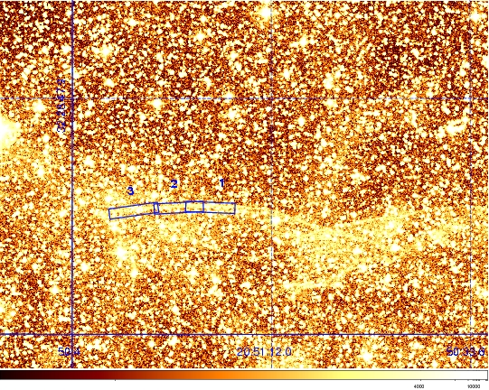
Figure 1.— Image of the northern Cygnus Loop showing filaments 1-3.

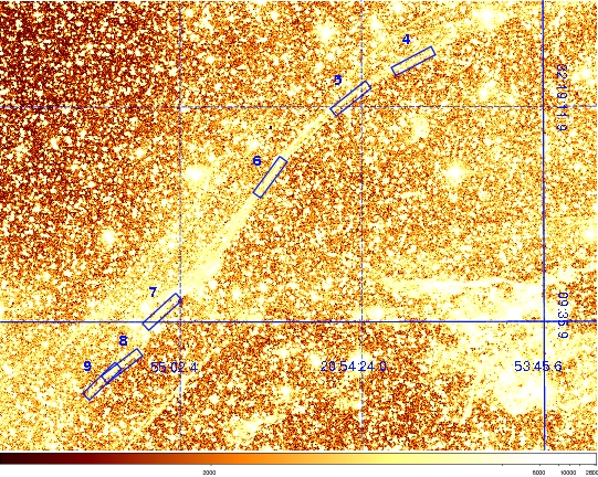
Figure 2.— Image of the northeastern Cygnus Loop showing filaments 4-9.

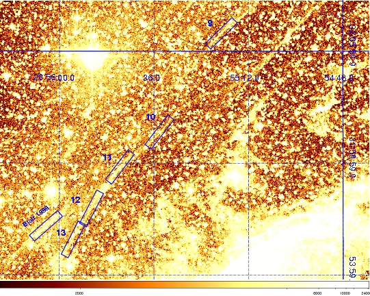
Figure 3.— Image of the northeastern Cygnus Loop showing filaments 9-13.

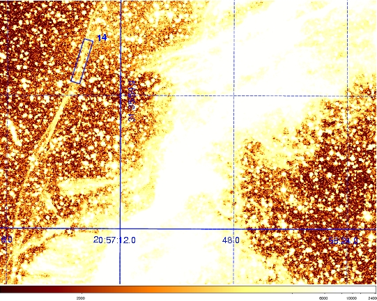
Figure 4.— Image of the northeastern Cygnus Loop showing filament 14.

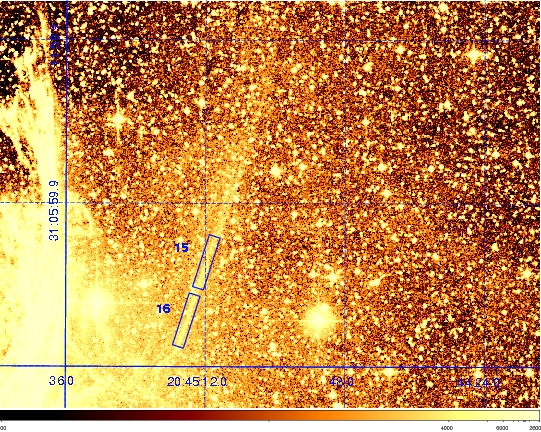
Figure 5.— Image of the western Cygnus Loop showing filaments 15 and 16.

Image of the eastern Cygnus Loop showing filaments 17 and 18.

labeled by a filament number which increments with decreasing declination. We adopted the following H$\alpha$ filament selection criteria applicable to both POSS-I and POSS-II images:

$\bullet$ Filaments must be bright relative to the local background.

$\bullet$ Selected filaments must be continuous with no local branching structure.

$\bullet$ Filaments must not precede another shock wave or strong optical emission within 100″ to provide an extractable ROSAT PSPC post-shock region for X-ray temperature analysis.

$\bullet$ A region enclosing a filament is not overwhelmed by stars.

$\bullet$ Filament geometry appears to be rigid and planar over both epochs allowing for uniform shock expansion in one dimension.

Each filament is hand selected and both epochs of images are reduced as described in $\S$ 2.1 to align the shock along the image axis. Rectangular regions 25″ $\times$ 120″ parallel to and enclosing the filament in both epochs are selected for proper motion analysis. Within this region we extract slices which cross the shock but omit sub-regions containing stars. This method of avoiding stars ensures that the brightness of the propagating shock will dominate its surroundings in the selected sub-regions. Figure 7 shows a typical example of the region selection process just described. The black rectangular regions of length 25″ track shock propagation and omit stars. These black regions are stacked while regions enclosed by white bars are discarded to collect all starless sub-regions. A bootstrap method randomly selects half of the rows within these starless sub-regions to sample over the length of the filament. For both POSS epochs, pixel values are summed down each column of sampled slices parallel to the shock, covering the 25″ region width. A one-dimensional cross-correlation of the totaled rows between both POSS epochs determines an optimal offset corresponding to the shock propagation. The bootstrap process just described is repeated 1000 times to provide a proper motion distribution and a statistical error estimate. The number of starless pixel rows did not exceed 600 with a required minimum of 200, ensuring well over 1000 possible combinations for bootstrap analysis. Figures 8 and 9 show an example of a proper motion distribution after 1000 trials and a plot of best-fit proper motions for a single iteration based on maximization of the correlation coefficient, respectively.

Table 2 lists proper motion measurements for each filament with 90$\%$ confidence errors according to the standard deviation of the randomly sampled distribution (see Figure 8). The time elapsed between POSS-I and POSS-II observations is 14,284 days (39.1 years). Proper motions over this timeline range from 2$\farcs$7 to 5$\farcs$4. We also give the conservative upper limit to the shock speed, $v_{s}$, obtained from the upper limit to the proper motion (proper motion plus uncertainty) and the upper limit to the distance of the background star given by Blair et al. (2008) of 576+61 = 637 pc. Matching filament locations ($\alpha$, $\delta$) with corresponding proper motions in Figures 1-6 demonstrates continuity of shock propagation along the rim of the Cygnus Loop and consistency of our measurements. Suitable filaments were restricted to the inner perimeter of H$\alpha$ emission to permit extraction of post-shock regions from ROSAT X-ray data. The post-shock gas must not

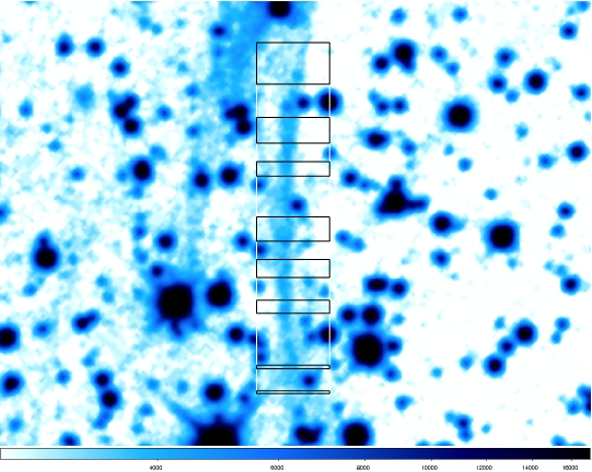
Figure 6.— Typical region selection process across an H$\alpha$ filament. The shock is aligned along the image axis and enclosed by a 25″ $\times$ 120″ rectangular region. The black sub-regions are selected for analysis. The sub-regions enclosed by the white lines are dominated by stars; therefore, they are not extracted for proper motion analysis. Identical sub-regions are extracted for both POSS epochs and the columns of the remaining starless regions are totaled for cross-correlation comparisons. This selection process is specific to filament 7.

encounter a trailing blast wave within $\sim$ 100″ to validate the assumption of ionization equilibrium required by our X-ray temperature analysis. While there are numerous, well-defined H$\alpha$ filaments delineating the northeastern Cygnus loop, we only measure proper motions of those where the post-shock gas has adequate time to reach thermal and ionization equilibrium, allowing us to constrain cosmic ray to gas pressure.

3.1.1 Proper Motion Uncertainty

The statistical uncertainties in the proper motions are determined by the measurement procedure to be 0$\farcs$1 to 0$\farcs$2 for all but one of the filaments. Additional systematic uncertainty could arise from the cross registration of the images from the different epochs, though that error should be small because of the large number of stars used in the cross correlation. Indeed, we have compared the positions of individual stars in the different epochs and find them to differ by considerably less than an arcsecond. It is also possible that changes in brightness among different regions within an unresolved filamentary structure (see Blair et al. 1999) could cause errors in the proper motion. We expect such errors to be small, and measurement of 18 positions limits the impact of any such errors. Thus while there is a small systematic error, it is unimportant because the uncertainties in temperature and distance dominate.

We can also compare with other proper motion determinations. Shull and Hippelein (1991) reported proper motions of 1$\farcs$3 to 14$\farcs$6 century^-1, with the latter value for a Balmer line filament close to our position 14, and Hester et al. (1986) found 7″ per century for two Balmer line filaments in the northeast, one of which was observed by Blair et al. (1999). Blair et al. observed a non-radiative H$\alpha$ filament in the Cygnus Loop ($\alpha_{J2000}=20^{h}56^{m}2^{s}.7,~{}\delta_{J2000}=31^{\circ}56\arcmin 39\farcs 1$) propagating into relatively dense neutral gas (see Figure 3). The filament proper motion was measured as 3$\farcs$6 $\pm$ 0$\farcs$5 by comparing POSS-I and Hubble Space Telescope (HST) images taken $\sim$ 44.3 years apart using stars as stationary reference points. However, the two reference stars used changed

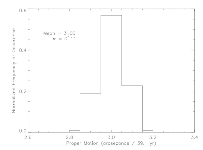
Figure 7.— Histogram distribution of proper motion measurements after 1000 bootstrap iterations. The bins are 0$\farcs$1 wide and the results are normalized to unity. The 90$\%$ confidence range in proper motion is represented by $\sigma$, given by multiplying the standard deviation by 1.645. This distribution is specific to filament 7.

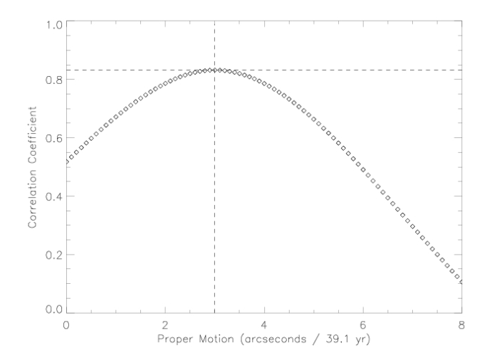
Figure 8.— Spread in correlation coefficient for one iteration between sampled POSS-I and POSS-II sub-regions contributing to the histogram in Figure 8. Maximization of the correlation coefficient determines the optimal proper motion of the filament. This distribution is specific to filament 7.

apparent position by 0$\farcs$5 and 0$\farcs$2, increasing proper motion uncertainty. We measured this same filament with the method described in $\S$ 3.1 by combining POSS-I and two different POSS-II observations taken on 1992 July 24 and 1995 August 25 yielding proper motions of 2$\farcs$6 $\pm$ 0$\farcs$1 and 3$\farcs$1 $\pm$ 0$\farcs$1, respectively. Assuming a constant shock speed, we extrapolate these measurements to 3$\farcs$0 and 3$\farcs$2 at the time of the 1997 November 16 HST observation. These two proper motion measurements and that of Blair et al. (1999) were made relative to the POSS-I 1953 June 15 plate, providing three independent measurements. Given that these results are within the limits presented in Blair et al. (1999) when reference star position changes are included, we consider our proper motion methodology justified. Although the HST image reveals intricate substructure, if we assume that the substructure of a particular filament has not dramatically changed over the POSS epochs, the poor resolution of the POSS plates smoothes these features and should give accurate results.

3.2. Post-Shock Temperature from ROSAT Spectral Fitting

We extracted PSPC spectra of four 25″ $\times$ 120″ strips stacked behind and parallel to each filament for measurements of post-shock gas temperature behavior over 100″. The single-temperature models apec and raymond show low post-shock temperature in the first $\sim$ 25″ behind each filament. Within the 100″ post-shock region, the fitted temperature is consistently lower within the 25″ region immediately behind the shock in agreement with Raymond et al. (2003). This suggests departure from ionization equilibrium immediately following the shock because the gas has had insufficient time to ionize.

We show below that the post-shock gas reaches ionization equilibrium after 25″, so we extracted PSPC X-ray spectra of a 75″ $\times$ 120″ region extending from 25″ to 100″ behind each filament. Corresponding background regions were selected outside of the X-ray shock front and scaled, and source and background regions reduced as discussed above ($\S$ 2.2). Figures 10-12 show the locations of extracted PSPC X-ray regions for all of the H$\alpha$ filaments we considered, where north is at the top and east is toward the left.

All of our spectral fits used the XSPEC model phabs to account for absorption of interstellar gas along the line of sight combined with a hot plasma X-ray emission model. The nominal interstellar column density value was $N_{H}=1.5\times 10^{20}\rm~{}cm^{-2}$, but it was allowed to vary in all model fits (Raymond et al., 2003; Decourchelle et al., 1997). For all the soft X-ray fits presented in this paper, $N_{H}$ is constrained within $\sim 1-5\times 10^{20}\rm~{}cm^{-2}$. The $kT_{e}$ and $N_{H}$ parameters in the model are highly (and negatively) correlated, in the sense that a very small change in the temperature yields a large change in $N_{H}$. The fluctuations in $N_{H}$ are likely not significant.

Ghavamian et al. (2000) measured H$\alpha$ velocity line widths of a non-radiative shock located between filaments 5 and 6 in the northeastern Cygnus Loop and found good electron-ion equilibration, $T_{e}/T_{i}\sim 0.7-1.0$, in the post-shock region. We have assumed $T_{e}=T_{i}$ throughout our analysis.

Single-temperature models and standard cosmic abundance assumptions are challenged by claims of bimodal temperature regions and depleted abundances (e.g. Nemes et al., 2008). Three fits were made to each PSPC X-ray spectrum: (i) a single-temperature fit assuming cosmic abundances (Anders & Grevesse, 1989), (ii) a single-temperature fit assuming depleted abundances, and (iii) a double-temperature fit assuming cosmic abundances. Depleted abundance fits fixed C, Mg, Al, Si, Ca, Fe, and Ni to 10$\%$ cosmic values on the basis that these elements are locked up in grains. Other abundances were fixed to cosmic values.

Table 3 lists the resulting best-fit temperatures and $\chi^{2}/\nu$ values using the XSPEC models:

(i)   phabs $\times$ apec,

(ii)  phabs $\times$ vapec,

(iii) phabs $\times$ (apec + apec),

while Table 4 lists the same parameters using the XSPEC models:

(i)   phabs $\times$ raymond,

(ii)  phabs $\times$ vraymond,

(iii) phabs $\times$ (raymond + raymond).

Tables 3 and 4 compare the apec and raymond models to determine the sensitivity of the cosmic ray to gas pressure ratio for slightly different X-ray temperature fits. $T_{\rm cos}$ and $T_{\rm dep}$ refer to temperature fits to models (i) and (ii), respectively. $T_{\rm low}$ and $T_{\rm high}$ are the bimodal temperatures from model (iii). Figures 13-15 show typical spectral fits for apec models (i), (ii), and (iii).

Temperature estimates are required for calculations of the cosmic ray to gas pressure ratio downstream. The double-temperature models consistently produce better fits based on $\chi^{2}$ statistics, and $T_{\rm low}$ remains continuous and consistent along ajacent filaments. However, there is no glaring physical reason to require two downstream temperatures. Hester et al. (1994) discuss how reflection of a blast wave from a dense cloud will enhance the temperature, and this may apply to the parts of the Cygnus Loop where the optical emission is bright, but we have avoided those complicated areas for this analysis. As discussed below, temperatures also depend on the assumed set of elemental abundances. We estimate the post-shock electron temperature as $T_{\rm cos}$ from the fits assuming cosmic abundances since they best represent the data. Lower limits on temperature are taken as $T_{\rm low}$ from the double-temperature models, as this gives conservative lower limits to the gas pressure. Cosmic ray to gas pressure is inferred and an upper limit is calculated based on these temperatures and measured proper motions. Temperatures from both apec and raymond models are independently analyzed for all 18 post-shock regions as a consistency check on temperature measurements.

3.2.1 X-Ray Temperature Uncertainty

The derivation of temperatures from X-ray data, especially low-resolution X-ray data such as that provided by ROSAT, is fraught with systematic errors. In this section, we attempt to quantify some of those errors.

Our extraction regions were chosen to provide at least 2,500 good x-ray events in each, so that the statistical errors are minimal.

We have made two assumptions in our fitting: equilibrium ionization, and cosmic abundances.

To investigate these, we produced spectra using the shock code of Cox and Raymond (1985) for a shock with $v_{s}=350~{}\mathrm{km~{}s^{-1}}$, which is typical of the velocities shown in Table 2, and a pre-shock density of 0.25 $\rm cm^{-3}$, which is typical of values determined from X-ray and UV observations (e.g., Raymond et al. 2003). We then integrated the surface brightness to distances which correspond to 25, 50, 75, and 100″ behind the shock. The resulting spectra were multipled by a photoelectric absorption model with $N_{\mathrm{H}}=1.5\times 10^{20}~{}\mathrm{cm^{-2}}$, convolved with the ROSAT response, and used with the XSPEC fakeit command to generate Poisson-sampled random spectra consistent with the shock model. We did this for both cosmic and depleted abundances.

We then fit these spectra with a cosmic abundance, single temperature raymond model, assuming equilibrium ionization. We find that for the cosmic abundance cases, the fitted temperature underestimated the true input temperature by 3%, which is a small effect. The first zone, within 25″ of the shock, had a much lower fitted temperature. Accordingly, in our fitting of the Cygnus Loop data, we have ignored the first 25″ bin.

Similarly, if we model a shock with depleted abundances, we find the spectrum is harder than with cosmic abundances. This is because much of the 1/4 keV band flux is provided by lines of Si, Mg, and Fe, while the 3/4 keV band flux at these shock speeds and temperatures is provided mostly by O and Ne which are undepleted even in dusty interstellar plasmas. Fitting such a spectrum with a model which presumes cosmic abundances will overestimate the temperature to produce the harder spectrum. However, the model allows the column density of neutrals along the line of sight to vary, and this can compensate and even overcompensate for the excess emission in the soft band predicted by the cosmic abundance model, so that the temperature can be underestimated. Overall, we find that fitting a depleted shock spectrum to a cosmic abundance equilibrium model underestmates the temperature by about 11%.

The large quantity of atomic physics data which go into simulations of the spectra of hot, collisional plasmas all have uncertainties as well. In order to assess these effects, we have fit the spectra with both the apec (Desai et al. 2005, Smith et al. 2001) and raymond (Raymond and Smith 1977, as updated) models. There is a systematic difference in the fitted temperatures of single-temperature, cosmic abundance models, in the sense that the raymond model gives a fitted temperature about $0.15\pm 0.05$ keV lower than the apec model does. This is probably because apec includes only emission lines for which reliable atomic data are available, while raymond includes emission lines which must be present, but for which the atomic data are more uncertain. This mainly affects the Mg, Si, S and Fe lines in the 1/4 keV band.

Accordingly, we discuss lower limits to the electron temperatures. We use the low temperatures from the two-temperature, cosmic abundance fits as conservative lower limits to the temperature and therefore to the gas pressure. Even so in many cases we find that they imply upper limits to the cosmic ray pressure which are negative, a clearly unphysical situation.

3.3. Other Temperature determinations for the Cygnus Loop

The Cygnus Loop is one of the most studied supernova remnants in the Galaxy, and each X-ray observatory in turn has observed it. Each observatory has its own strengths and weaknesses, and the ensemble of results helps to constrain the systematics of any one observation. Many of these observations cover the area we study, with special attention on the NE rim.

Miyata et al. (2007) analyze Suzaku observations of a field in the NE. Their superior spectral resolution in the 0.3–2 keV band shows many lines of elements such as C, N, O, Ne and Mg. They fit two-temperature models to the spectra and find the higher temperature component, which is constrained by the lines in the spectrum, has $kT$ greater than about 0.2 keV.

Tsunemi et al. (2007) analyze data from a series of XMM-Newton pointings across the Cygnus Loop from NE to SW. They also fit two-temperature models to narrow concentric slices of the remnant. Their lower temperature (which they identify as the forward shock) is always greater than $kT$ = 0.2 keV.

The Chandra observatory has also observed the NE rim. Katsuda et al. (2008) report fits to the XSPEC vpshock model, which allows for nonequilibrium ionization effects, and variable abundances. They also obtain fitted temperatures uniformly in excess of 0.2 keV.

It therefore seems that these high temperatures are quite robust features of the X-ray emission from the NE rim of the Cygnus Loop. Chandra’s high spatial resolution, XMM-Newton’s large collecting area and Suzaku’s superior spectral resolution all lead to the same conclusion we obtain from the

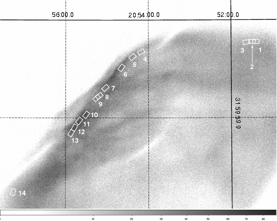
Figure 9.— ROSAT PSPC image of the northeastern Cygnus Loop showing locations of the X-ray source extraction regions behind filaments 1-14.

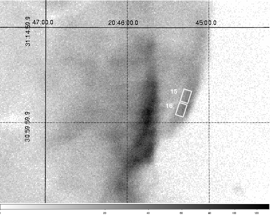
Figure 10.— ROSAT PSPC image of the western Cygnus Loop showing locations of the X-ray source extraction regions behind filaments 15 and 16.

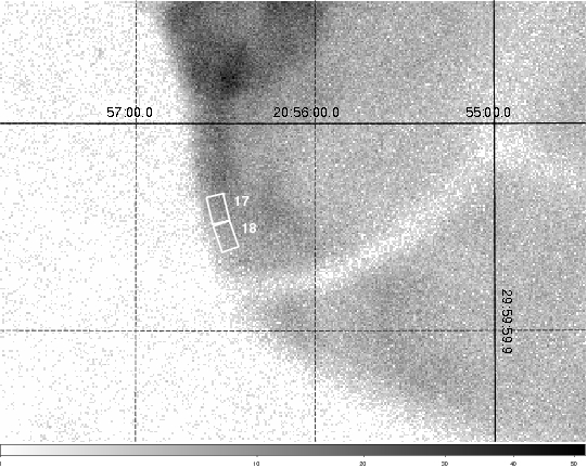
Figure 11.— ROSAT PSPC image of the eastern Cygnus Loop showing locations of the X-ray source extraction regions behind filaments 17 and 18.

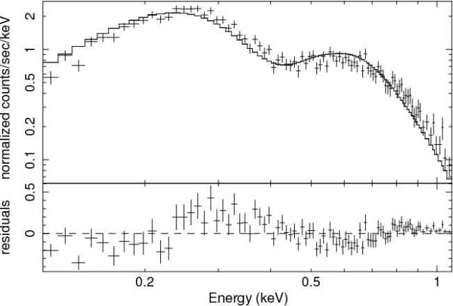
Figure 12.— Representative example of a ROSAT PSPC single-temperature apec model fit with abundances fixed to cosmic values. In most cases, this model was statistically better than the depleted model. This fit is specific to filament 7.

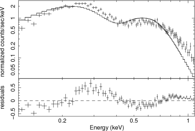
Figure 13.— Representative example of a ROSAT PSPC single-temperature apec model fit with C, Mg, Al, Si, Ca, Fe, and Ni abundances depleted to 10$\%$ cosmic values and fixed. The rational for depletion is that these elements may be locked up in grains. This fit is specific to filament 7.

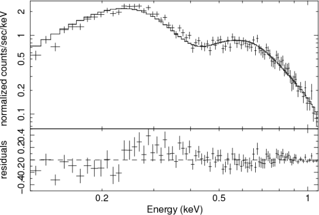
Figure 14.— Representative example of a ROSAT PSPC double-temperature apec model fit with abundances fixed to cosmic values. In most cases, a bimodal temperature distribution was statistically significant, providing motivation to investigate this in future works. This fit is specific to filament 7.

ROSAT data: $kT$ values of 150 eV or higher are ubiquitous in the non-radiative filaments of the Cygnus Loop.

3.4. Distance

The distance to the Cygnus Loop is a substantial uncertainty, and our measurements can be used to obtain a lower limit to the distance. Minkowski (1958) obtained the canonical value of 770 pc from the velocity ellipse and proper motions, though Braun and Strom (1986) used the same data to obtain 460$\pm$160 pc using the mean expansion velocity instead of the extreme. Shull & Hippelein (1991) obtained a distance of 600 pc based on Fabry-Perot scans of a large number of fields in the Cygnus Loop, but with a range of 300 to 1200 pc. Sakhibov and Smirnov (1983) also compared proper motions and radial velocities to obtain an estimate of 1400 pc. Though the method of comparing radial velocities and proper motions relies only upon the assumptions of symmetric expansion and radial motion, it leads to a wide range of distance estimates.

An independent distance estimate by Blair et al. (1999) combined the proper motion of a single filament with a shock speed obtained from spectroscopic analysis and fits to shock models. They derived a distance of 440 pc with a range of 340 to 570 pc. Their method assumed that $P_{CR}/P_{G}$ is zero, and a larger value would imply a higher shock speed and therefore a larger distance. This proper motion had a relatively large uncertainty because of the possible motions of the two reference stars.

The most solid limit on the distance to the Cygnus Loop comes from Blair et al. (2008). They used FUSE to observe an sdO star and found strong high velocity O VI absorption lines matching the O VI emission in the adjacent nebulosity. A fit to the FUSE spectrum provided the temperature and surface gravity of the star, indicating a distance of 576$\pm$61 pc. The upper end of this range, 637 pc, should be a firm upper limit to the distance of the Cygnus Loop. Distances to sdO stars are generally difficult to determine, but the spectral fits should give an accurate temperature. The uncertainty in the surface gravity probably dominates the 10% uncertainty in the distance.

3.5. Analyses of other Balmer line shocks in the Cygnus Loop

Several of the Balmer line shocks at the periphery of the Cygnus Loop have been studied previously. The shock observed by Blair et al. has been observed extensively at optical and UV wavelengths (e.g. Raymond et al. 1983; Fesen & Itoh 1985; Long et al. 1992; Hester et al. 1994). We do not include it here (except to check our proper motion measurements; $\S$ 3.1.1) because it is too slow to produce X-ray emission. However, it fits in with our analysis in that the shock speed is estimated to be 150 to 190 $\rm km~{}s^{-1}$ and the proper motion is around two thirds the typical values we measure for the X-ray producing shocks.

The filament corresponding to our positions 15 and 16 was studied by Raymond et al. (1980) and Treffers (1981), who measured an H$\alpha$ line width corresponding to a shock speed faster than 170 $\rm km~{}s^{-1}$. The filament corresponding to our positions 17 and 18 was discussed by Fesen, Kwitter & Downes (1992) and Graham et al. (1995). The latter paper finds that the Balmer line filament in the region we observed is indeed the blast wave, rather than part of the shock structure refracted around the dense cloud just to the north.

Detailed studies of a position in the northeast have been made by Ghavamian et al. (2001) and Raymond et al. (2003). We have not included this exact region because two filaments overlap near there, but it lies between our regions 5 and 6. Ghavamian et al. obtained H$\alpha$ and H$\beta$ profiles and found nearly equal proton and electron temperatures ($T_{e}/T_{i}>0.7$ and a shock speed of 235 to 395 $\rm km~{}s^{-1}$. Raymond et al. (2003) combined those results with UV spectra from FUSE and the Hopkins Ultraviolet Telescope. They found further evidence for near equilibration among the particle species, with an oxygen kinetic temperature near that of hydrogen ($T_{O}<2.5T_{p}$). They also analyzed the ROSAT X-ray spectrum, finding 0.14 $<T_{e}<$0.2 keV. They also observed a bright rim about 25″thick which they attributed to enhanced emission in the 0.25 keV band due to non-equilibrium ionization. They found that a 350 $\rm km~{}s^{-1}$ shock matches the optical, UV and X-ray data. This speed combined with the average of the proper motions of positions 5 and 6, 3$\farcs$75, would give a distance of 750 pc. It should be mentioned, however, that van Adelsberg et al. (2008) computed models of H$\alpha$ profiles in non-radiative shocks and were unable to simultaneously match the broad line component width and the broad to narrow intensity ratio reported by Ghavamian et al.

4. Cosmic Ray to Gas Pressure

The proper motion and temperature measurements described above, combined with a distance to the Cygnus Loop, allow calculation of the upper limit to the cosmic ray to gas pressure ratio downstream.

Taking the perspective of the shock front, momentum conservation applies to the pre- and post-shocked gas:

$$\rho\frac{\partial{\bf v}}{\partial t}+\rho({\bf v}\cdot{\bf\nabla})\bf{v}+{\bf\nabla}P+\rho{\bf\nabla}\phi=0$$

Assuming a steady solution exists, ignoring the gravitational force term resulting from a field, $\phi$, and applying the continuity equation $\rho v=$ constant, the momentum equation becomes,

$$\rho v\frac{dv}{dx}+\frac{dP}{dx}=\frac{d}{dx}(P+\rho v^{2})=0.$$

This translates into a statement of constant momentum flux across the shock, allowing us to equate pressure terms,

$$P_{1}+\frac{B_{1}^{2}}{8\pi}+\rho_{1}v_{s}^{2}=P_{CR}+P_{G}+\frac{B_{2}^{2}}{8\pi}+\rho_{2}v_{2}^{2},$$

where $v_{s}$ is shock speed, $\rho$ is density, $P_{CR}$ is cosmic ray pressure originating in a dissipative shock environment, $P_{G}$ is downstream gas pressure, $B^{2}/8\pi$ is magnetic pressure, and the subscripts 1 and 2 represent conditions in the pre- and post-shock regions, respectively. We assume the ram and downstream pressures dominate, neglecting the ambient gas pressure and interstellar magnetic field. Assuming the case of a strong shock with adiabatic exponent $\gamma=\frac{5}{3}$ where $n_{2}/n_{1}=4$ and $v_{2}=\frac{1}{4}v_{s}$, along with the equations of state $\rho_{1}=n_{1}m$ and $P_{G}=n_{2}kT_{2}$, we derive:

$$1+\frac{P_{CR}}{P_{G}}=\frac{3mv_{s}^{2}}{16kT_{2}}=\frac{3m\mu^{2}d^{2}}{16kT_{2}\Delta t^{2}},$$

where $T_{2}$ is the mean post-shock temperature. We assume ionization equilibrium exists, and that $T_{2}=T_{e}=T_{i}$ (Ghavamian et al., 2000). We calculate shock velocities assuming only a tangential component, $v_{s}=v_{\theta}=\frac{\mu d}{\Delta t}$, where $\frac{\mu}{\Delta t}$ is the angular propagation across the sky over a particular timescale (i.e. proper motion) and d is distance to the Cygnus Loop. Adopting cosmic abundances with n(He)/n(H) = 0.098 (Anders & Grevesse, 1989), the mean mass per particle behind the shock, m, is determined by dividing the weighted molar mass per nucleus by the average number of particles per nucleus. The cosmic ray to gas pressure ratios presented in this paper are computed according to the equation derived above. We note that the compression factor of 4 may be an underestimate if cosmic ray pressure significantly impacts the gas dynamics, decreasing the post-shock flow speed relative to the shock, but as will be seen, we are primarily interested in low efficiency shocks. We neglect line of sight velocity components in our calculations, assuming the shock velocity is mostly perpendicular to the line of sight. We note that the appearance of multiple propagating shock layers is an artifact of our two-dimensional perspective. Instead, the complicated three-dimensional structure of the Cygnus Loop is wavy, warped, and sheet-like (Raymond et al. 2003). Cosmic ray to gas pressure ratios were calculated by combining proper motion and temperature measurements with an adopted distance of 576 $\pm$ 61 pc, obtained from a distance upper limit to a background subdwarf OB star (Blair et al., 2008).

Note that the density has dropped out of the equations. The results we present here do not depend upon the ambient density, which is not very well known.

Table 2 lists best-fit values and upper limits of $P_{CR}/P_{G}$ for all 18 filaments calculated independently with the apec and raymond ionization equilibrium temperature fits. To obtain conservative upper limits, we have used the upper limits to the shock speed $v_{s}$ from Table 2 based on upper limits to the proper motions and the upper limit to the distance of 637 pc (Blair et al. 2008). We find several negative values for $P_{CR}/P_{G}$. This result is unphysical and requires further investigation. For all instances of negative pressure ratios we set $P_{CR}/P_{G}$ to zero and derive a minimum distance estimate to the Cygnus Loop based on our proper motion and temperature uncertainties.

5. Discussion

Inspection of the derived cosmic ray to gas pressure equation emphasizes the importance of constraining proper motion, distance, and temperature to infer tight upper limits on $P_{CR}/P_{G}$. $P_{CR}/P_{G}$ scales with the square of the shock speed, given by the product of proper motion and distance. In general, the upper limits indicate a small value for the ratio, and in some cases it is formally negative.

In the context of the discussions of the uncertainties given above, it is clear that the proper motion measurements cannot account for the unphysical values of $P_{CR}/P_{G}$. Most distance estimates are significantly smaller than the 637 pc we have adopted as the nominal upper limit, and it seems like a strain to make the distance large enough ($\sim 1$ kpc) to make all the upper limits to $P_{CR}/P_{G}$ positive. However, it may be possible given the general uncertainties in SdO star distances.

Therefore, we conclude that the heart of uncertainty likely lies in post-shock temperature measurements and electron-ion thermal equilibration assumptions. Assuming ionization equilibrium and that shock velocity measurements are reasonably accurate, we require lower post-shock electron temperatures than measured from our ROSAT PSPC X-ray spectral fits. The fits based on the Raymond & Smith (1977) code give temperatures about 10% lower than those using APEC, but that is several times too small to explain the discepancy.

5.1. Heating by Thermal Conduction

There is another possible way out of the discrepancy. We have assumed that $T_{e}=T_{i}$ behind the shock, and it is possible that $T_{e}>T_{i}$. However, such behavior is not seen in shocks in the interplanetary medium, and there is no obvious physical reason for such electron heating in the shock. Ghavamian et al. (2006) describe a wave heating mechanism that would produce particle temperatures somewhat higher than observed here, but $T_{p}$ from Ghavamian et al. (2001) and a higher $T_{e}$ would then require a large value of $V_{s}$.

An interesting alternative is electron heating by thermal conduction from gas farther behind the shock. A number of papers have explored the global structure of SNRs with thermal conduction (e.g., Slavin & Cox 1992; Cox et al. 1999; Shelton et al. 1999). We can obtain an observational estimate from X-ray observations. Nemes et al. (2008) show the variation of $T_{e}$ with radius in the northeastern Cygnus Loop based on XMM spectra, with a gradient of 0.05 keV over a distance of 0.07 times the shock radius, or $\nabla T\sim 1.8\times 10^{-13}~{}\rm K~{}cm^{-1}$. This implies a volumetric heating rate of about $3.4\times 10^{-22}~{}\rm erg~{}cm^{-3}~{}s^{-1}$, which could heat the gas by about $3\times 10^{5}$ K as it travels over the 100″ region we analyze. Thus the true post-shock temperature could be somewhat lower than the X-ray temperatures we measure by approximately the amount required for $P_{CR}$ greater than zero. The above estimate requires a temperature gradient parallel to the magnetic field, so it could not be correct everywhere. However, only 7 of the 18 positions show $P_{CR}$ nominally smaller than zero.

6. Summary

Constraining $P_{CR}/P_{G}$ in supernova shocks is important for assessing the efficiency of energy dissipated by the SNR into accelerating cosmic rays. We combine measured proper motions with temperatures derived from X-ray spectra and an upper limit to the distance to obtain upper limits to $P_{CR}/P_{G}$. We measured proper motions and post-shock temperatures of 18 faint nonradiative H$\alpha$ filaments in the Cygnus Loop. Proper motion measurements of filaments based on image matching and correlation techniques yield continuous results over extended shock regions. Post-shock electron temperatures from X-ray fits are higher than expected if the current 576 $\pm$ 61 pc distance measurement to the Cygnus Loop is accurate.

We conclude that 1) $P_{CR}/P_{G}$ is small, 2) the distance to the Cygnus Loop must be close to or even larger than the upper limit given by the apparent distance to a star that lies behind the SNR, 3) uncertainties in the temperature derived from X-ray spectra might dominate the uncertainties in the analysis, and 4) thermal conduction from hotter interior gas could alter the immediate post-shock temperature enough to account for the observations.

Future work will focus on constraining post-shock temperature and investigating the validity of ionization equilibrium on a more global scale along the northeastern Cygnus Loop, and placing tighter constraints on the distance to the Cygnus Loop.

This work is supported in part by the National Science Foundation Research Experiences for Undergraduates (REU) and Department of Defense Awards to Stimulate and Support Undergraduate Research Experiences (ASSURE) programs under Grant no. 0754568 and by the Smithsonian Institution.

We acknowledge generous data policies of the Space Telescope Science Institute, for digitizing and archiving the Palomar Observatory Sky Surveys, and the High Energy Astrophysics Space Astronomy Archival Research Center (HEASARC) at the NASA/Goddard Space Flight Center, for making the ROSAT data available. The Digitized Sky Survey was produced at the Space Telescope Science Institute under U.S. Government grant NAG W-2166. The images of these surveys are based on photographic data obtained using the Oschin Schmidt Telescope on Palomar Mountain and the UK Schmidt Telescope. The plates were processed into the present compressed digital form with the permission of these institutions. RJE acknowledges support from NASA contract NAS8-03060 (the Chandra X-ray Center) to the Smithsonian Astrophysical Observatory.

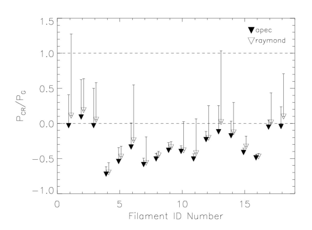
Figure 15.— Mapping filaments by their numbers defined in Figures 1-6 corresponding to $P_{CR}/P_{G}$ best fits with error bars extending to the calculated upper limit. Results for XSPEC model fits apec are shown as filled symbols and raymond results are shown as open symbols. Groupings of local filament regions cluster around similar $P_{CR}/P_{G}$ values. Filaments 4-13, which delineate the northeastern rim of the Cygnus Loop, appear to show $P_{CR}/P_{G}$ values consistent with zero.

Table 1 

Cygnus Loop ROSAT  PSPC Observation Parameters

Name	$\alpha_{J2000}$	$\delta_{J2000}$	Date	Exposure
			(UT)	(ksec)
rp500034a01	20 55 02.4	+32 07 12.0	1992 Nov 04	12.0
rp500267n00	20 56 21.6	+30 24 00.0	1993 Nov 14	9.24
rp500268n00	20 45 40.8	+31 02 24.0	1994 Jun 03	9.75

Table 2 

Proper Motion and $P_{cr}/P_{g}$ Values for Selected H$\alpha$ Filaments

Filament ID	$\alpha_{J2000}$	$\delta_{J2000}$	Proper Motion	$v_{max}$	$(P_{CR}/P_{G})_{\rm apec}$	$(P_{CR}/P_{G})^{MAX}_{\rm apec}$	d${}^{\rm MIN}_{\rm apec}$	$(P_{CR}/P_{G})_{\rm raymond}$	$(P_{CR}/P_{G})^{MAX}_{\rm raymond}$	d${}^{\rm MIN}_{\rm raymond}$
			arcsec / 39.1 yr	km s-1			pc			pc
1	20 51 23.9	32 24 22.5	5$\farcs$1 $\pm$ 0$\farcs$2	403	-0.032	0.408	537	0.111	1.274	422
2	20 51 29.9	32 24 21.8	5$\farcs$4 $\pm$ 0$\farcs$2	433	0.091	0.625	500	0.190	0.637	498
3	20 51 38.6	32 24 14.5	5$\farcs$2 $\pm$ 0$\farcs$2	416	-0.032	0.501	520	0.053	0.582	507
4	20 54 13.1	32 21 14.0	2$\farcs$7 $\pm$ 0$\farcs$2	225	-0.723	-0.616	1028	-0.698	-0.560	960
5	20 54 26.2	32 19 36.5	3$\farcs$4 $\pm$ 0$\farcs$2	278	-0.543	-0.344	786	-0.473	-0.325	775
6	20 54 43.4	32 16 04.0	4$\farcs$1 $\pm$ 0$\farcs$2	333	-0.337	-0.004	638	-0.239	0.550	512
7	20 55 06.3	32 10 03.8	3$\farcs$0 $\pm$ 0$\farcs$1	240	-0.587	-0.496	897	-0.561	-0.193	709
8	20 55 14.7	32 07 38.9	3$\farcs$4 $\pm$ 0$\farcs$1	274	-0.507	-0.428	843	-0.456	-0.397	821
9	20 55 18.9	32 06 58.0	3$\farcs$7 $\pm$ 0$\farcs$1	294	-0.384	-0.275	748	-0.338	-0.259	740
10	20 55 34.6	32 01 40.2	3$\farcs$5 $\pm$ 0$\farcs$1	279	-0.400	-0.317	771	-0.383	0.026	629
11	20 55 44.9	31 59 43.8	3$\farcs$1 $\pm$ 0$\farcs$2	254	-0.507	-0.432	845	-0.424	0.066	617
12	20 55 51.8	31 57 34.8	4$\farcs$0 $\pm$ 0$\farcs$2	319	-0.231	-0.115	677	-0.203	0.253	569
13	20 55 56.5	31 55 55.1	4$\farcs$2 $\pm$ 0$\farcs$7	375	-0.120	0.256	568	0.020	1.034	447
14	20 57 20.2	31 37 32.4	4$\farcs$3 $\pm$ 0$\farcs$1	342	-0.176	0.030	628	-0.127	0.299	559
15	20 45 11.9	31 03 50.0	3$\farcs$4 $\pm$ 0$\farcs$1	272	-0.415	-0.351	791	-0.329	-0.182	704
16	20 45 15.3	31 01 41.4	3$\farcs$3 $\pm$ 0$\farcs$1	264	-0.492	-0.443	854	-0.470	-0.428	842
17	20 56 37.4	30 08 34.4	4$\farcs$5 $\pm$ 0$\farcs$1	358	-0.054	0.049	622	0.013	0.434	532
18	20 56 34.8	30 06 27.8	4$\farcs$8 $\pm$ 0$\farcs$1	379	-0.044	0.237	573	0.099	0.707	…

Table 3 

X-ray Spectral Fit Parameters with the apec Model

Filament ID	Tcos	NH,cos	$(\chi^{2}/\nu)_{\rm cos}$	Tdep	$(\chi^{2}/\nu)_{\rm dep}$	Tlow	Thigh	$(\chi^{2}/\nu)_{\rm double}$
	eV	$10^{20}\rm~{}cm^{-2}$		eV		eV	eV
1	187${}^{+6}_{-6}$	2.4${}^{+0.2}_{-0.2}$	1.65	162${}^{+10}_{-7}$	3.37	137	536	1.13
2	192${}^{+7}_{-6}$	2.4${}^{+0.2}_{-0.2}$	1.80	198${}^{+10}_{-9}$	3.01	137	602	1.28
3	198${}^{+7}_{-6}$	2.5${}^{+0.2}_{-0.2}$	1.44	230${}^{+10}_{-10}$	2.47	137	336	1.16
4	190${}^{+6}_{-6}$	2.3${}^{+0.2}_{-0.2}$	0.96	194${}^{+9}_{-8}$	1.86	157	454	0.85
5	181${}^{+5}_{-4}$	2.5${}^{+0.2}_{-0.2}$	1.48	159${}^{+8}_{-6}$	3.21	140	605	1.06
6	179${}^{+4}_{-2}$	2.1${}^{+0.1}_{-0.1}$	2.33	151	5.75	132	380	1.60
7	154${}^{+5}_{-4}$	2.6${}^{+0.2}_{-0.2}$	2.22	119	5.95	136	541	1.53
8	170${}^{+12}_{-4}$	1.2	1.26	118${}^{+4}_{-4}$	3.44	156	661	1.06
9	159${}^{+6}_{-5}$	1.7${}^{+0.2}_{-0.2}$	1.45	115${}^{+4}_{-4}$	3.63	141	656	1.14
10	146	2.1	5.59	80.8	10.7	135	…	3.90
11	139	1.9	5.07	80.8	9.92	135	690	3.95
12	145${}^{+3}_{-3}$	1.1${}^{+0.1}_{-0.1}$	2.91	80.8	7.18	136	685	1.55
13	139	1.7	5.03	80.8	9.34	133	863	3.40
14	159${}^{+8}_{-7}$	1.8${}^{+0.3}_{-0.3}$	1.48	115${}^{+7}_{-4}$	3.14	135	727	0.89
15	140${}^{+3}_{-5}$	2.1${}^{+0.2}_{-0.2}$	2.81	80.8	5.24	135	812	2.29
16	150${}^{+4}_{-4}$	2.4${}^{+0.1}_{-0.1}$	1.02	86.8	1.91	148	692	1.03
17	152${}^{+13}_{-9}$	4.2${}^{+0.6}_{-0.7}$	1.19	146${}^{+9}_{-7}$	1.91	145	159	1.24
18	169${}^{+11}_{-20}$	3.8${}^{1.1}_{-0.5}$	1.32	155${}^{+23}_{-10}$	1.88	138	633	1.24

Table 4 

X-ray Spectral Fit Parameters with the raymond Model

Filament ID	Tcos	NH,cos	$(\chi^{2}/\nu)_{\rm cos}$	Tdep	$(\chi^{2}/\nu)_{\rm dep}$	Tlow	Thigh	$(\chi^{2}/\nu)_{\rm double}$
	eV	$10^{20}\rm~{}cm^{-2}$		eV		eV	eV
1	163${}^{+7}_{-8}$	3.5${}^{+0.5}_{-0.4}$	1.69	453${}^{+22}_{-20}$	1.57	84.8	360	0.93
2	176${}^{+8}_{-3}$	3.0${}^{+0.2}_{-0.4}$	1.89	485${}^{+27}_{-24}$	1.70	136	702	1.27
3	182${}^{+6}_{-5}$	2.9${}^{+0.2}_{-0.2}$	1.47	487${}^{+26}_{-24}$	2.31	130	356	1.13
4	174${}^{+6}_{-11}$	2.8${}^{+0.6}_{-0.3}$	1.03	444${}^{+20}_{-16}$	1.93	137	448	0.84
5	157${}^{+6}_{-5}$	3.6${}^{+0.4}_{-0.3}$	1.51	432${}^{+10}_{-10}$	2.19	136	776	1.06
6	156${}^{+4}_{-4}$	3.2${}^{+0.2}_{-0.2}$	2.17	427${}^{+9}_{-15}$	3.18	84.8	266	1.28
7	145${}^{+3}_{-2}$	3.5${}^{+0.2}_{-0.2}$	2.02	372${}^{+12}_{-12}$	2.85	84.9	292	1.09
8	154${}^{+4}_{-4}$	2.1${}^{+0.2}_{-0.2}$	1.16	430${}^{+6}_{-9}$	2.29	148	…	1.08
9	148${}^{+4}_{-4}$	2.5${}^{+0.2}_{-0.2}$	1.34	415${}^{+17}_{-17}$	2.02	138	…	1.11
10	142	2.8	5.19	373${}^{+10}_{-9}$	3.23	89.9	539	2.60
11	119${}^{+5}_{-5}$	3.6${}^{+0.4}_{-0.3}$	4.61	326${}^{+8}_{-8}$	2.32	71.9	449	1.67
12	140${}^{+3}_{-1}$	1.9${}^{+0.1}_{-0.2}$	2.58	379${}^{+10}_{-9}$	2.08	96.1	425	1.04
13	120${}^{+5}_{-5}$	3.2${}^{+0.4}_{-0.3}$	4.63	366${}^{+11}_{-10}$	2.98	82.1	627	1.84
14	150${}^{+6}_{-5}$	2.6${}^{+0.3}_{-0.3}$	1.34	431${}^{+21}_{-23}$	1.17	107	670	0.84
15	122${}^{+9}_{-7}$	3.7${}^{+0.6}_{-0.5}$	2.66	114${}^{+4}_{-5}$	2.83	107	704	1.81
16	144${}^{+4}_{-3}$	0.9${}^{+0.2}_{-0.1}$	1.02	133${}^{+3}_{-5}$	1.16	144	145	1.06
17	142${}^{+6}_{-5}$	5.3${}^{+0.5}_{-0.6}$	1.22	143${}^{+9}_{-6}$	1.39	106	693	1.03
18	147${}^{+10}_{-7}$	5.2${}^{0.7}_{-0.8}$	1.32	150${}^{+12}_{-10}$	1.52	…	147	1.39