Kinetic roughening in a realistic model of non-conserved interface growth

Abstract

We provide a quantitative picture of non-conserved interface growth from a diffusive field making special emphasis on two main issues, the range of validity of the effective small-slopes (interfacial) theories and the interplay between the emergence of morphologically instabilities in the aggregate dynamics, and its kinetic roughening properties. Taking for definiteness electrochemical deposition as our experimental field of reference, our theoretical approach makes use of two complementary approaches: interfacial effective equations and a phase-field formulation of the electrodeposition process. Both descriptions allow us to establish a close quantitative connection between theory and experiments. Moreover, we are able to correlate the anomalous scaling properties seen in some experiments with the failure of the small slope approximation, and to assess the effective re-emergence of standard kinetic roughening properties at very long times under appropriate experimental conditions.

1 Introduction

Many natural and technological growth systems exist whose dynamics results from the interplay between diffusive transport of aggregating units within dilute phase, and their attachment at a finite rate to a condensed growing cluster. Examples abound particularly within Materials Science, e.g. in the production of both amorphous (through Chemical Vapor Deposition [1] or Electrochemical Deposition [2]), and of epitaxial (by Molecular Beam Epitaxy [3]) thin films. Still, a similar variety of surface morphologies can be found in diverse systems, such as e.g. bacterial colonies [4], to the extent that universal mechanisms are expected to govern the evolution of these non-equilibrium systems [5]. Moreover, many times it is not matter, but e.g. heat that is transported, but obeying precisely the same constitutive laws (one-sided solidification).

The objects of interest in the time evolution of these systems are the morphological properties of the aggregate which is produced. Thus, a variety of behaviors ensue, such as pattern formation and evolution [5], and surface kinetic roughening [6], whose understanding has driven a large effort within the Statistical Mechanics and Nonlinear Science communities. In this context, continuum models have played a prominent role, due to the compact description they typically provide of otherwise very complex phenomena, and their ability to explore generic or universal system properties [7]. For the diffusive growth systems mentioned above, the simplest continuum formulation takes the form of a moving boundary problem in which particle diffusion in the dilute phase is coupled with a boundary condition in which the growth velocity of the aggregate is prescribed as, roughly, the fraction of random walkers that finally stick irreversibly to it. Thus, the evolution of a growing surface from a vapor or the electrochemical growth of a metallic deposit under galvanostatic conditions can be described by the same nonlinear system of stochastic differential equations (see Sec. 2 for details).

Electrochemical deposition (ECD) has been widely studied mainly due to the apparent simplicity of the experimental setup and the capability to control different relevant physical parameters. Most of the studies in ECD address the growth of quasi-two dimensional fractal aggregates. This can be achieved by confining a metallic salt between two parallel plates with a small separation between them. Thus, although the formulation of the problem can be accurately posed in order to include all the physical mechanisms involved, its solution is far from trivial (actually it cannot be obtained even in the deterministic case). Moreover, the numerical integration of the corresponding equations often involves the use of complex algorithms that take into account the motion of the boundary and which, in practice, are difficult to implement. Besides this intrinsic complexity, the role of fluctuations and their inclusion in the numerical scheme is still an open question. In the present context, the interplay among different transport or electrochemical mechanisms is not clear and the predictive power of different models is limited to the description of the concentration of cations in the solution or the qualitative morphologies of the fractal aggregates [8, 9].

In this scenario, two possibilities arise from a theoretical point of view. On the one hand, one can try to obtain as much information as available from customary perturbation methods. Thus, linearization, Green’s function projection techniques or weakly nonlinear expansions provide important information at both short (linear regime) and asymptotic times [10]. Briefly, this approach allows to explore the physics of the problem in the so-called small slopes approximation. On the other hand, one can try to integrate numerically a more computationally efficient version of the moving boundary problem in order to accurately determine the validity of the approximations in the model formulation, and also to gain insight into the intermediate time regimes.

This second approach can be achieved by the introduction of an equivalent phase-field model [11] version of the moving boundary problem. Phase-field models have been successfully introduced in the last few years to understand moving boundary problems which are harder to integrate numerically (or in combination with discrete lattice algorithms [12]). Moreover, they have become a paradigmatic representation of multi-phase dynamics whose application ranges from solidification [13, 14] or Materials Science [15, 16, 17, 18] to Fluid Mechanics [19, 20] or even Biology [21].

The aim of this paper is to provide a quantitative picture of non-conserved growth in which material transport is of a diffusive nature. Working for the case of ECD, we will focus on two important and complementary tasks: assessing the validity of the effective small-slopes (interfacial) theories, and the emergence of unstable aggregates that cannot be described by single valued functions. More importantly, we will show that our model is capable to provide both a qualitative and a quantitative picture of growth by electrochemical deposition. In particular, our present study allows us to provide more specific reasons for the experimental difficulty in observing kinetic roughening properties of the Kardar-Parisi-Zhang universality class, in spite of theoretical expectations. Finally, we will see that the frequently observed anomalous scaling properties arise in this class of systems associated with the failure of the single-valued description of the interface, and may yield asymptotically to standard scaling behavior, provided a well defined aggregate front reappears.

Our paper is organized according to the following scheme: in Sec. II we introduce our model and discuss in depth the relationship between its defining parameters and physical ones. In Sec. III, we discuss the validity of the small slope approximation and conclude on the need of a full phase-field description of the problem. Section IV collects the results of a detailed comparison with specific ECD experiments that allows us to derive a consistent picture of pattern formation within our non-conserved growth system. Finally, Sec. IV concludes the paper by summarizing our main findings and collecting some prospects and open questions.

2 Continuum model of galvanostatic electrodeposition

Recently we have proposed a stochastic moving boundary model to describe the morphological evolution of a variety of so-called diffusive growth systems [10]. This is a large class of systems in which dynamics arises as a competition between supply of material from a dilute phase through diffusion, and aggregation at a growing cluster surface through generically finite attachment kinetics. The deterministic limit of the model has a long history in the field of thin film growth by Chemical Vapor Deposition [22, 23, 24], where diffusing species are electrically neutral, conceptually simplifying the theoretical description. Naturally, in the case of aggregate growth by electrochemical deposition (ECD) in galvanostatic (constant current) conditions, the situation is more complex due to the existence of two diffusing species (anions and cations) and an imposed electric field. Nonetheless, an explicit mapping of the corresponding dynamical equations can be made to the CVD system, by means of the following assumptions: (i) zero fluid velocity in a thin electrochemical cell; (ii) anion annihilation at the anode, whose position is located at infinity, namely, the aggregate height is much smaller than the distance separating the electrodes; (iii) electroneutrality away from the electrodes; (iv) zero anion flux at the cathode. Within these assumptions, the model ECD system takes the form [10]

$$\partial_{t}c = D\nabla^{2}c-\nabla\cdot{\bf q},$$ (1)

$$D\partial_{n}c\Big{|}_{\zeta} = k_{D}(c-c^{0}_{eq}+\Gamma\kappa+\chi)\Big{|}_{\zeta}+{\bf q}\cdot{\bf n},$$ (2)

$$V_{n} = \Omega\,\Big{[}D\partial_{n}c-\nabla_{s}\cdot{\bf J}_{s}-{\bf q}\cdot{\bf n}-\nabla_{s}\cdot{\bf p}\Big{]},$$ (3)

$$\lim_{z\rightarrow\infty} \hskip-14.22636ptc(x,z;t)=c_{a}.$$ (4)

In (1)-(4) the field $c$ is the cation concentration $C$, rescaled by a quantity $R_{c}$ that depends on the diffusivity and the mobility of the two species (cations and anions). Specifically, $R_{c}$ is the ratio between the ambipolar diffusion coefficient $D$ and the constant $t_{c}$, defined by

$$D=\frac{\mu_{c}D_{a}+\mu_{a}D_{c}}{\mu_{c}+\mu_{a}}\qquad t_{c}=\frac{\mu_{c}}{\mu_{c}+\mu_{a}},$$ (5)

where $\mu_{a}(\mu_{c})$, $D_{a}(D_{c})$ are the anion (cation) mobility and diffusivity, respectively. Other parameters in Eqs. (1) to (4) are $c^{0}_{eq}=R_{c}C_{a}\exp[z_{c}F\eta/(RT)]$, $c_{a}=R_{c}C_{a}$, $\Gamma=\gamma/(RT)$, $\Omega=M/\rho=(1-t_{c})/C_{a}$, and the mass transport coefficient $k_{D}=J_{0}\exp[-bz_{c}F\eta/(RT)]/(z_{c}FC_{a}R_{c})$, where $C_{a}$ is the initial cation concentration, held fixed at infinity, $M$ is the metal molar mass and $\rho$ the aggregate mean density, $T$ is temperature, $\gamma$ is the aggregate surface tension, $R$ is the ideal gas constant and $F$ is Faraday’s constant, $ez_{c}$ is the cation charge, $J_{0}$ is the exchange current density in equilibrium, and $\eta$ is the overpotential from which a surface curvature contribution in the corresponding Butler-Volmer boundary condition [2, 25, 26] has been singled out, parameter $b$ estimating the asymmetry of the energy barrier related to cation reduction.

Eq. (1) describes cation diffusion in the cell, with a noise $\mathbf{q}$ term that describes fluctuations in the (conserved) diffusive current. Eq. (2) is a mixed boundary condition at the aggregate surface $\zeta$ that determines the efficiency at which the cation flux leads to actual aggregation. It originates from the standard Butler-Volmer condition, and allows for a noise term $\chi$ accounting for fluctuations in attachment. In this equation $\partial_{n}$ represent the derivative along the normal component $\bf{n}$ of the interface. Eq. (3) computes the growth velocity along the local normal direction $V_{n}=\mathbf{V}\cdot\mathbf{n}$, incorporating the contributions from the diffusive current mediated by the boundary condition (2), as well as from other diffusive currents at the surface, $\mathbf{J}_{s}$, in which fluctuations are described by the noise term $\mathbf{p}$. The standard choice is that of surface diffusion [27, 28], $\nabla_{s}\cdot\mathbf{J}_{s}=\Omega^{2}\nu_{s}D_{s}\gamma(k_{B}T)^{-1}\nabla_{s}^{4}\zeta$, where $\nu_{s}$ is the surface concentration of diffusing species and $D_{s}$ is their surface diffusivity. Here, $\nabla_{s}^{2}$ denotes the surface Laplacian. Finally, the stochastic moving boundary problem is complete with the boundary condition (4) prescribing a fixed cation concentration at the anode.

In the above model of ECD, in principle all parameters can be estimated in experiments. This is also the case for the noise terms: indeed, their amplitudes can be shown to be functions of the physical parameters above, once we take the noises as Gaussian distributed numbers that are uncorrelated in time and space, and make a local equilibrium approximation [10]. The mathematical problem posed by Eqs. (1) to (4) is analytically very hard to work with. However, substantial progress can be made by means of a small slope, approximation $|\nabla\zeta|\ll 1$ [29, 30, 10]. This approach allows to obtain a closed evolution equation for the Fourier modes $\zeta_{k}(t)$ of disturbances of the surface height away from a flat interface. Generically, such an equation takes the form [29, 30, 10]

$$\partial_{t}\zeta_{k}(t)=\omega_{k}\zeta_{k}(t)+\frac{V}{2}\mathcal{N}[\zeta]_{k}+\eta_{k}(t),$$ (6)

where $\eta_{k}(t)$ is an additive noise term including both conserved and non-conserved contributions, and $\mathcal{N}[\zeta]_{k}$ is the Fourier transform of $\mathcal{N}[\zeta]=(\partial_{x}\zeta)^{2}$, namely, of the celebrated Kardar-Parisi-Zhang (KPZ) nonlinearity that is the landmark of non-conserved interface growth. Here, $V$ is the mean velocity of a flat interface, while the dispersion relation $\omega_{k}$ is a function of wave-vector magnitude $k$ that provides the (linear) rate of growth or decay of a periodic perturbation $\zeta_{k}(t)$ of the flat solution. In the simplest long-wavelength limit, the dispersion relation becomes a polynomial in $|k|$, with two important limits, namely

$$\omega_{k}=\left\{\begin{array}[]{lc}V|k|[1-(d_{0}l_{D}+B\Omega/2D)k^{2}]-B\Omega k^{4},&k_{D}\to\infty\quad\mbox{MS}\\ (Dk_{D}\Delta/V)(k^{2}-l_{D}d_{0}[1-(Vd_{0}/D)^{1/2}]^{-1}k^{4}),&k_{D}<\infty\quad\mbox{KS}\end{array}\right.$$ (7)

where $B=\Omega^{2}\gamma\nu_{s}D_{s}/(RT)$, and $\Delta=1-d_{0}/l_{D}$ with $d_{0}=\Gamma\Omega$ the capillary length and $l_{D}=D/V$ the diffusion length, the condition $d_{0}\ll l_{D}$ applying in most physical cases. As we see from (7), in all cases the dispersion relation predicts a morphological instability in which there is a band of linearly unstable Fourier modes whose amplitudes grow exponentially in time. One of these modes grows at a faster rate than all the other, providing the selection of a characteristic length-scale in the surface and formation of a periodic pattern. However, some features of the instability change as a function of the mass transfer parameter $k_{D}$. Thus, when attachment kinetics is very fast ($k_{D}\to\infty$) the dispersion relation has the classic shape of the Mullins-Sekerka (MS) instability. In this case, Eq. (6) is non-local in space, as a reflection of the strong implicit shadowing effects associated with diffusion. In the case of slow kinetics and, as long as $d_{0}<l_{D}$, we still have a morphological instability, but of a local nature, Eq. (6) becoming the celebrated (stochastic) Kuramoto-Sivashinsky (KS) equation in real space.

Remarkably, the KPZ nonlinearity is able to tame the morphological instabilities in (6) and induce, albeit after relatively long transients, kinetic roughening properties at long length scales [10]. These are those of the KPZ equation for slow attachment kinetics, while they correspond to a different universality class for $k_{D}\to\infty$. Thus, one would expect KPZ scaling for a wide range of parameters, which has indeed been found experimentally within ECD growth [31], but not with the generality that was expected [30, 32]. One possibility is that the crossovers induced by the instabilities are so long lived as to prevent actual asymptotic scaling from being accessed by experiments. Such a possibility seems to occur in conceptually similar growth techniques, such as Chemical Vapor Deposition [33, 34]. However, standard symmetry arguments [6] lead to the expectation of generic KPZ behavior for such non-conserved growth phenomena as provided by ECD systems. Thus, in order to understand this disagreement, in the next section we undertake a detailed comparison between the small slope approximation and ECD growth experiments.

3 Dispersion Relation and Small Slope Approximation

The simplest way to improve upon the analytical results of the previous section is to realize that Equation (7) merely provides a long-wavelength approximation of the exact linear dispersion relation for the moving boundary problem. We can consider the full shape of the dispersion relation, that turns out to be an implicit (rather than explicit) function of wave-vector, namely [35]

$$\left(1+\left[1+\hat{\omega}_{k}+\hat{k}^{2}\right]^{1/2}\right)\left(2-\frac{V}{2k_{D}}\hat{\omega}_{k}-\frac{d_{0}}{2l_{D}}\hat{k}^{2}\right)=\hat{\omega}_{k}+4,$$ (8)

where $\hat{k}=2Dk/V$ and $\hat{\omega}_{k}=4D\omega_{k}/V^{2}$. Using this formula, we can see the extent to which surface kinetics modifies the functional form of the linear dispersion relation. Actually, several experimental studies of ECD have already tried to estimate the functional form of the dispersion relation in compact aggregates. An example taken from the literature is the growth of quasi-two-dimensional Cu and Ag branches by de Bruyn [36, 37]. In [37], the branches grow in the cathode due to the electrodeposition of ions created from the CuSO₄ aqueous solution. The analysis of the early stages of the branch growth allows the author to fit the experimental dispersion relation to

$$\omega_{k}=\frac{q|k|(1-rk^{2})}{1+sk},$$ (9)

where $q$, $r$ and $s$ depend on the properties of the electrolyte and the deposited metal, the ion concentration, and the applied current. From the reported data and figures in Ref. [37] we can extract the information summarized in Table 1, where we also include data from the experiments in [38, 39].

Parameter	Ref. [37]	Ref. [38]	Ref. [39]
$C_{a}$ [mol/cm3]	$1\times 10^{-4}$	$2\times 10^{-3}$	$5\times 10^{-4}$
$I$ [mA]	$1.4225$	NR	NR
$J_{0}$ [mA/cm2]	$3\times 10^{-2}$	$3\times 10^{-2}$	$3\times 10^{-2}$
$J$ [mA/cm2]	$11.16$	NR	65.00
$D_{c}$ [cm2/s]	$0.720\times 10^{-5}$	$0.720\times 10^{-5}$	$0.720\times 10^{-5}$
$D_{a}$ [cm2/s]	$1.065\times 10^{-5}$	$1.065\times 10^{-5}$	$1.902\times 10^{-5}$
$z_{c}$	$2$	2	2
$V$ [cm/s]	$3.45\times 10^{-4}$	$\approx 1.00\times 10^{-6}$	$4.87\times 10^{-4}$
$l_{D}$ [cm]	$2.49\times 10^{-2}$	$\simeq 8.59$	$2.15\times 10^{-2}$

Table 1: Experimental parameter values estimated from Refs. [37] (second column), [38] (third column), and [39] (4th. column). NR stands for not reported.

We need to supplement these values with reasonable estimates for the capillary length, $d_{0}$ and the mass transfer coefficient, $k_{D}$. We estimate $d_{0}$ from the experiments by Kahanda et al. [38] (and summarized in Table 1; see also below) and we rescale this value for the right concentration to $d_{0}=2\times 10^{-5}$ cm. Finally, $k_{D}$ can be obtained from the location of the maximum in the dispersion relation. Thus we can estimate $k_{D}$ to be in the range (due to the experimental uncertainty) $4.44-5.56\times 10^{-4}$ cm/s.

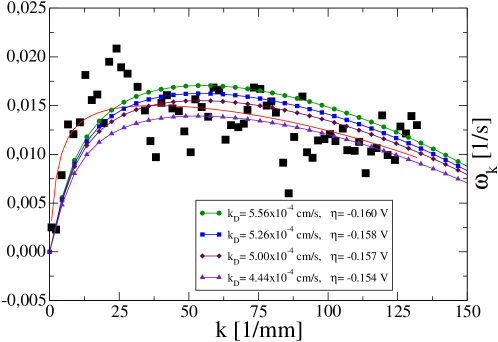
Figure 1: Linear dispersion relation, $\omega_{k}$, of Cu electrodeposition. Squares provide the experimental values taken from Ref. [37], and the red line is the fit to (9) made in this reference. The other lines are numerical solutions of (8) using the parameters in the second column in Table 1 for different values of $k_{D}$ as indicated in the legend.

These data are compatible with the assumptions made in the derivation of the moving boundary problem introduced in Ref. [10]. For instance, the diffusion length is larger than the branch width (typically $0.1$ mm in these experiments) but the mean growth velocity is comparable to the mass transport coefficient, and surface kinetics become relevant. For this reason, the growth process is not diffusion limited and the dispersion relation is very different from the Mullins-Sekerka one. Similarly, the estimate for $k_{D}$ implies that the applied overpotential $\eta$ varies between $-0.160$ V and $-0.154$ V, which are plausible enough. With this information we can now proceed to recast the experimental results in Ref. [37] as shown in Fig. 1. The agreement between our theory (8) and experiment is remarkable, taking into account that we are not performing any fit of the data. Moreover, the long wavelength approximations (7) are not able to fit the experimental data.

We have performed a numerical integration of an improved version of Eq. (6) in which the full linear dispersion relation (8) is employed, using a stochastic pseudospectral scheme, see e.g. [40, 10]. Results are shown in Fig. 2 for the time evolution of the surface roughness $W(t)$ (root mean square deviation) and the surface structure factor or power spectral density (PSD), $S(k,t)=\langle|\zeta_{k}(t)|^{2}\rangle$, of the surface height, $\zeta(x,t)$. As we see, the roughness increases very fast (close to $W(t)\sim t^{1.8}$) within an intermediate time regime, after which saturation to a stationary value is achieved.

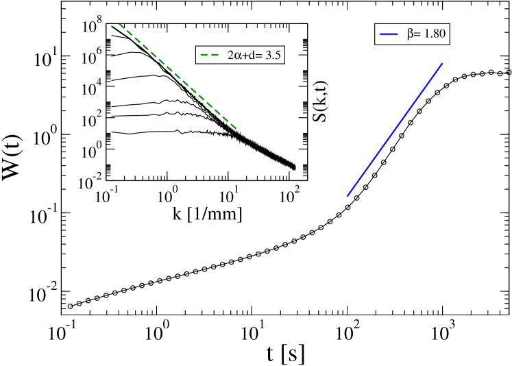
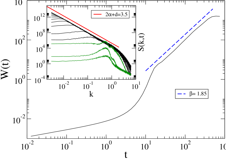
Figure 2: Time evolution of the surface roughness and PSD (insets) using (6) with $\omega_{k}$ given by (8) (left panel) and (10) for $\mu=0.75$ (right panel).

As for the time evolution of the PSD curves, they follow a standard Family-Vicsek (FV) behaviour [6], leading to a global roughness exponent $\alpha=1.25$, from the asymptotic behaviour $S(k)\sim k^{-(2\alpha+d)}$ for a 1D ($d=1$) interface. The time evolution of the interface height in real space can be appreciated in movie 1 in the supplementary material. As is clear from the images, an initially disordered interface develops mound-like structures that coarsen with time, leading to a long time super-rough morphology. This is inconsistent with the above expectation of KPZ scaling for the present case since, taking into account the values of $V$ and $k_{D}$, a KS behavior is expected for (8). In the inset of Fig. 3 we show the full dispersion relation (8) for sufficiently small values of wave-vector at which behaviour is indeed of the KS type. This apparent contradiction can be explained taking into account that such a KS shape (that holds for length scales in the cm range) cannot be observed in practice for the physical length-scales that are accessible in the experiment.

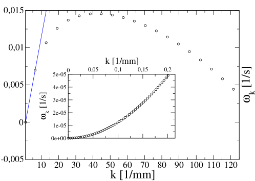
Figure 3: Full linear dispersion relation as shown in Fig. 1 for $k_{D}=5\cdot 10^{-4}$ cm s^-1. For the meaning of the solid line see the main text. The inset is a zoom showing the $\omega_{k}\sim k^{2}$ behaviour for sufficiently small $k$ values.

As seen in the figure, the effective behavior of the dispersion relation is not of the KS type but, rather, $\omega_{k}$ behaves (sub)linearly for the smallest accesible $k$ values. This is made explicit in the main panel of Fig. 3, where a straight line is shown for reference at the smallest wave-vectors. Thus, for all practical purposes the linear dispersion relation that is experimentally operative does not behave as $\sim k^{2}$ but, rather, is closer to a form such as

$$\omega_{\mu}(k)=b_{\mu}|k|^{\mu}-b_{2}k^{2},$$ (10)

where $b_{\mu}$ and $b_{2}$ are positive, effective parameters, and $0<\mu\leq 1$.

Taking into account the previous paragraphs, we see that (10) summarizes the main features of the linear dispersion relation for many experimental systems, namely, (i) fast growth at the smallest available $k$ values, $\omega_{k}\sim|k|^{\mu}$, (ii) single finite maximum at intermediate $k$ values, and (iii) sufficiently fast decay at large wave-vectors, at least of the form $\omega_{k}\sim-k^{2}$ or faster (i.e. with a larger exponent value). Thus, a simple way to explore the dynamics as predicted by the small slope approximation with an improved dispersion relation consists in considering Eq. (6), but using (10) rather than (7). We have carried out such type of study for several values of $\mu$. For the sake of reference, movie 2 in the supplementary material shows the evolution of an interface obeying the KS equation, while movie 3 displays the analogous evolution but as described by Eq. (6) using the effective dispersion relation (10) for $\mu=0.75$. It is apparent that the latter resembles much more closely the dynamics associated with the full dispersion relation (8). Quantitative support is provided by the right panel of Fig. 2, where the evolution of the roughness and PSD is shown for Eq. (6) with (10) for $\mu=0.75$. In the inset, we can appreciate the formation of a periodic surface (signalled as a peak in the PSD) at initial times that grows very rapidly in amplitude, as confirmed by the exponential evolution of the global surface roughness $W(t)$, shown in the main panel of Fig. 2, for times $t\lesssim 15$. For long enough times, this peak smears out, once the lateral correlation length is larger than the pattern wavelength. That marks the onset for nonlinear effects that induce power-law behavior (kinetic roughening) both in the roughness and in the PSD, approximately as $W(t)\sim t^{1.85}$ and $S(k)\sim 1/k^{3.5}$, wherefrom we conclude that the associated critical exponents have values $\beta=1.85$ and $\alpha=1.25$ (thus, $z=\alpha/\beta=0.68$, not far from $z=\mu=0.75$, an exponent relation which at least holds for (10) when $\mu=1$ [10].) We find it remarkable that the KPZ nonlinearity is able to stabilize the initial morphological instability of Eq. (6) even in the case of a dispersion relation such as $\omega_{\mu=0.75}$ that induces such a fast rate of growth. Notice $z=0.68<1$ corresponds effectively to correlations building up at a rate that is even faster than ballistic. Moreover, the height profile develops values of the slope at long times that are no longer compatible with the $|\nabla\zeta(t)|\ll 1$ approximation that led to the derivation of Eq. (6) in the first place. This requires us to reconsider the original moving boundary problem from a different perspective.

4 Multivalued interfaces

In order to go beyond the small-slope approximation one has to face the numerical integration of the full moving boundary problem (1)-(4). As mentioned in the introduction, a method of choice to this end is the so-called phase-field or diffuse interface approach [11]. In this method, one introduces an auxiliary (phase) field $\phi(\mathbf{r},t)$ that is coupled to the physical concentration field $c(\mathbf{r},t)$ in such a way as to reproduce the original moving boundary problem asymptotically, within a perturbation expansion in the small parameter $\epsilon=W/l_{D}$. Here, $W$ denotes the typical size of the region within which the value of $\phi(\mathbf{r},t)$ changes between $\phi=-1$ in the vapor phase and $\phi=+1$ in the solid phase. The level set $\phi=0$ will thus provide the locus of the aggregate surface, avoiding the need of explicit front tracking. For our present physical problem, such an asymptotic equivalence has been recently established [35] for the following phase-field reformulation of the stochastic system (1)-(4),

$$\tau\partial_{t}\phi=W^{2}\nabla^{2}\phi-\partial_{\phi}\big{[}f(\phi)-\lambda ug(\phi)\big{]}+\sigma_{\phi},$$ (11)

$$\partial_{t}u=\nabla\cdot\left(Dq(\phi)\,\nabla u-\mathbf{j}_{at}\right)-\frac{1}{2}\partial_{t}h(\phi)-\nabla\cdot\boldsymbol{\sigma}_{u},$$ (12)

where, $u=\Omega(c-c^{0}_{eq})$, $\sigma_{\phi}$ and $\boldsymbol{\sigma}_{u}$ are noises whose variances are related to those of $\mathbf{q}$ and $\chi$ in (1)-(4) [35], and $f(\phi)$, $g(\phi)$, $q(\phi)$, and $h(\phi)$ are auxiliary functions that are conveniently chosen (in order to achieve asymptotic convergence) as $f(\phi)=\phi^{4}/4-\phi^{2}/2$, $g(\phi)=\phi-2\phi^{3}/3+\phi^{5}/5$, $q(\phi)=(1-\phi)/2$, and $h(\phi)=\phi$ [41]. Moreover, the current $\mathbf{j}_{at}$ generates a so-called anti-trapping flux that is needed for technical reasons related to convergence [41, 35], and can be taken as $\mathbf{j}_{at}=8^{-1/2}W(\partial_{t}\phi)\,\nabla\phi/|\nabla\phi|$. Given model (11)-(12), one can finally prove [35] its convergence to the original moving boundary problem in the thin interface limit $\epsilon\ll 1$, provided model parameters are related as

$$d_{0}=a_{1}\frac{W}{\lambda},$$ (13)

$$k_{D}^{-1}=a_{1}\left(\frac{\tau}{\lambda W}-a_{2}\frac{W}{D}\right),$$ (14)

where $a_{1}$ and $a_{2}$ are constants associated with the phase-field model, with values

$$a_{1} = 0.8839,$$

$$a_{2} = 0.6267.$$ (15)

There have been previous proposals of phase-field formulations of diffusive [42, 43, 44] (and ballistic [45, 44]) growth systems of the type of our moving boundary problem. However, in these works the phase-field equations are proposed on a phenomenological basis, rather than being connected with a physical moving boundary problem as in our case. Thus, quantitative comparison is harder to achieve, although many qualitative morphological features can indeed be retrieved.

We have performed numerical simulations of model (11)-(12) using physical parameter values that correspond to the experiments of Cu ECD by Kahanda et al. [38] (see parameters in Table 1), for different surface kinetics conditions. Representative morphologies are shown in Fig. 4, where the overpotential value is employed to tune the value of the kinetic coefficient $k_{D}$.

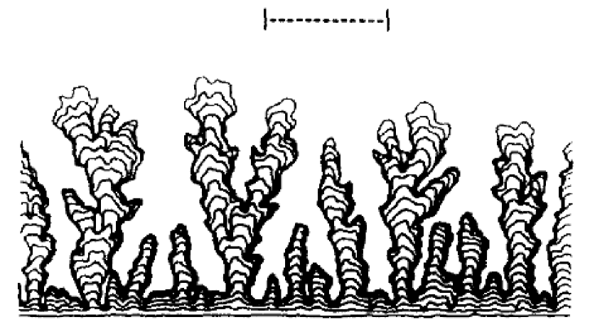
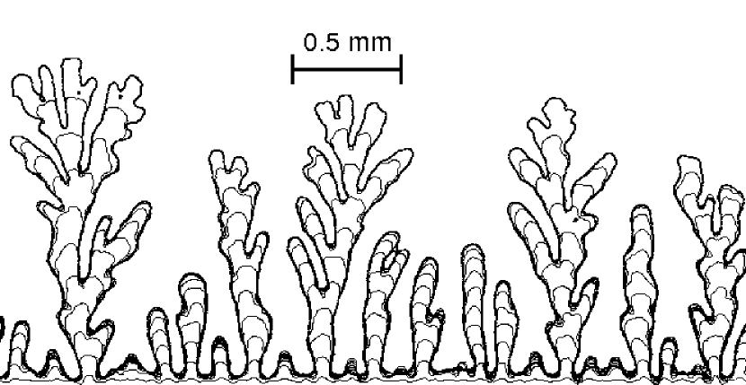
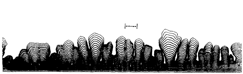
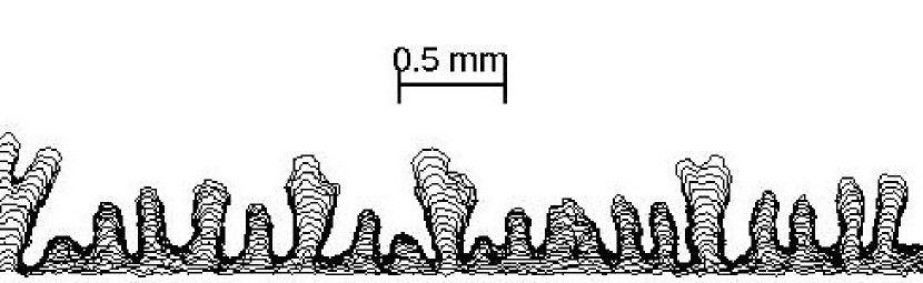
Figure 4: Comparison of morphologies from the experiments on CuSO₄ in Ref. [38] (left column, taken from the original paper by permission; reference bars represent 0.5 mm) and phase-field simulations using parameters in Table 1 (right column). Top row corresponds to fast kinetics ($\eta=-0.50$ V), and bottom row corresponds to intermediate kinetics ($\eta=-0.35$ V).

Notice that in Ref. [38] the average growth velocity is overestimated, having been measured in the nonlinear regime, which also overshoots the estimated value of the capillary length. For this reason, the value of the capillary length employed in our simulations (and provided in Table 1) is estimated as smaller than that in [38]. As we can see, for the faster kinetics case (upper row in Fig. 4), indeed the interface becomes multivalued already at early times, leading to a relatively open, branched morphology. As the overpotential increases (thereby decreasing the value of $k_{D}$, lower row), the morphology is still multivalued, but more compact. We would like to stress the large degree of quantitative agreement between the simulated and experimental morphologies.

Our phase-field model (and the corresponding moving boundary problem that it represents) has moreover a large degree of universality, in the sense that it can also reproduce quantitatively other ECD systems. An example is provided by Fig. 5, which shows simulations for ECD growth from a Cu(NO₃)₂ solution, as in Ref. [39], see experimental parameters in Table 1. This dense branching morphology corresponds to a fast kinetics condition for which the single valued approximation breaks down already for short times. Fig. 6 collects the time evolution of the surface roughness and of the PSD function for the same parameters as in Fig. 5.

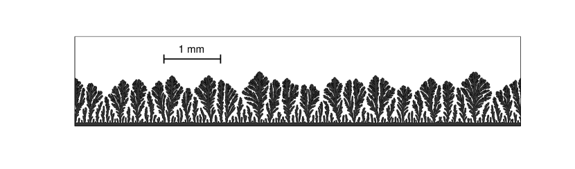
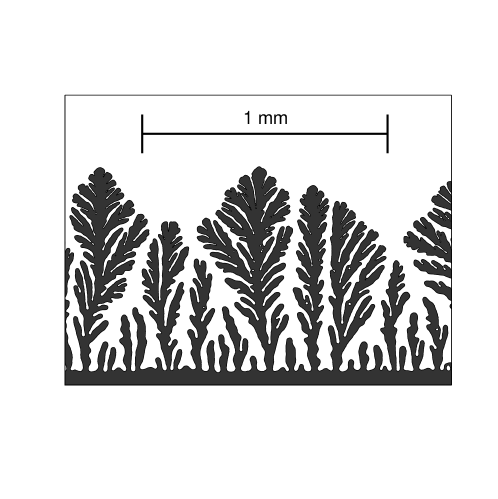
Figure 5: Simulated morphology using parameters as in the experiment of Ref. [39] on Cu(NO₃)₂, corresponding to a fast kinetics condition. Lower panel: zoom of a portion of the upper panel.

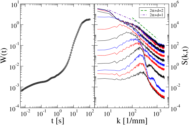
Figure 6: Numerical time evolution of the surface roughness (left panel) and PSD (right panel) for the same parameters as in Fig. 5. The PSD curves are for increasing times from bottom to top. Notice the time shift of the PSD curves for high values of $k$ (small length scales) signalling anomalous scaling, see the text for details. For reference, the dashed line has slope $-2$ while the dash-dotted line has slope $-1$.

The roughness grows rapidly within a transient regime, that is later followed by stabilization and rapid saturation to a stationary value. This result is similar to those obtained within the small slope approximation. However, the behavior of the PSD differs dramatically. Thus, for very small times the linear instability shows up in the finite maximum of the curves. For intermediate times the PSD’s shift upwards with time, a behaviour that is associated with anomalous kinetic roughening properties [8, 46] that contrasts with the standard FV scaling found above in which the PSD values are time independent for length scales that are below the correlation length. Note that at these intermediate times the single valued approximation does not describe the features of the interface at all. Actually, the single valued approximation to the height field (not shown) presents abundant large jumps that are possibly responsible for the effective anomalous scaling [47]. However, for sufficiently long times branches grow laterally closing the interbranch spacing, and the validity of the single valued approximation is restored. Thus, the PSD curves for the longest times again display Family-Vicsek behavior for the largest $k$ values. A crossover between $\alpha=0.5$ for small scales and $\alpha=0$ (log) for intermediate scales can be read off from the figure.

Note that, for the longest distances in our system, scale invariance seems to break down, since no clear power law can be distinguished for, say, $k<30$ mm${}^{-1}\simeq l_{D}^{-1}$. In order to properly characterize the behavior of the interface at these scales, simulations are required for system sizes that are much larger the diffusion length. We hope to report on this in the future.

5 Discussion and Conclusions

In this paper we have studied the physics of non-conserved growth from a diffusive source. We have focused on, both, morphological features and dynamical properties, making special emphasis in the emergence of a long time structure arising from a well characterized linearly unstable regime. Thus, we have dealt with the problem from two different but complementary points of view: the linearized dispersion relation obtained from the moving boundary description of the problem (as presented in Ref. [10]) and the use of a phase-field equivalent description of the full original physical system.

This complementary study has allowed us to understand the evolution of the problems in two well separated regimes: one at short times, well characterized by the linear dispersion relation, and another one at long times in which steep slopes may eventually develop and break down the simplistic description through a single valued height field. We want to emphasize that the comparison has been done quantitatively. Thus, in Sec. II we have shown how our theoretical predictions allow to explain some experimental results reported in [37]. At variance with the data analysis performed in this reference, our comparison is not based on a multidimensional fit of the parameters but arises, rather, from a prediction for the form of the dispersion relation compatible with the available experimental data.

In order to develop insight into the dynamics decribed by the complex full dispersion relation (8), we have proposed a simple description of the evolving interface in terms of an effective dispersion relation, in which the exponent $\mu$ of the destabilizing term comprises all the relevant information on the behavior of the morphological instability at the largest length scales accesible in the system. Hence, the simple description of the data given by Eq. (6) using (8) provides a promising testbed for future theoretical analysis of many problems sharing similar ingredients with ours. Another benefit of this characterization of the linear regime is to provide an explanation for the scarcity of experimental evidence of the celebrated KPZ scaling (or even its generalization for unstable systems given by the KS equation). As we have demonstrated, the difficulty of actually observing the experimental systems in the KPZ universality class is due to the fact that the physical conditions for the observation of that behavior cannot be fulfilled for realistic (experimentally motivated) values of the parameters, as they typically require system sizes that are beyond experimental feasibility.

Besides, with the help of the phase-field model we have also performed a systematic analysis of the experiments reported in [38]. Our comparison not only reproduces qualitatively well the morphologies obtained in those experiments but also predicts the existence of a scaling regime characterized by anomalous scaling. This anomalous scaling deserves further analysis but, preliminarily, can be understood in terms of the emergence of large slopes for times following appearance of overhangs and multivalued interfaces. As we have shown, our model sheds some light on the characterization of the experiments reported in Refs. [38, 39] and the role of the different mechanisms involved. The quantitative estimation of the parameters appearing in our theoretical framework leads also to remarkable agreement with the morphological structure of the observed deposits.

Finally, we want to stress that, although the formulation of the electrochemical deposition process with a phase-field theory has been addressed before in the literature [42, 43, 44, 45], our model is not constructed phenomenologically, but is, rather, an equivalent formulation of the physical equations (diffusion, electrochemical reduction at the cathode, etc.) that reduces to them in the thin-interface limit. In addition, our formulation allows us to do a quantitative comparison with experiments which is far from the capabilities of the mentioned theories. Notwithstanding, the promising results presented above still need more detailed comparison and analysis (through more extensive numerical experiments), which will be the aim of future work. This will focus particularly on the appearance of the anomalous scaling regime and, from the morphological point of view, on the influence, cooperation and/or competition of different physical mechanisms that are naturally included in our theory.

6 Acknowledgments

This work has been partially supported by MEC (Spain), through Grants No. FIS2006-12253-C06-01 and No. FIS2006-12253-C06-06, and by CAM (Spain) through Grant No. S-0505/ESP-0158. M. N. acknowledges support by the FPU programme (MEC) and by Fundación Carlos III.

References

References

- [1] K. Jensen and W. Kern, in Thin Film Processes II, edited by J. Vossen and W. Kern (Academic, Boston, 1991).
- [2] J. Bockris and A. Reddy, Modern electrochemistry (Plenum/Rosetta, New York, 1970).
- [3] A. Pimpinelli and J. Villain, Physics of Crystal Growth (Cambridge University Press, Cambridge, 1998).
- [4] M. Matsushita et al., Biofilms 1, 305 (2005).
- [5] P. Ball, The self-made tapestry: pattern formation in nature (Oxford University Press, Oxford, 1999).
- [6] A.-L. Barabási and H. E. Stanley, Fractal concepts in surface growth (Cambridge University Press, Cambridge, 1995).
- [7] R. Cuerno et al., Eur. Phys. J. Special Topics 146, 427 (2007).
- [8] M. Castro, R. Cuerno, A. Sánchez, and F. Domínguez-Adame, Phys. Rev. E 57, 2491 (1998).
- [9] M. Castro, R. Cuerno, A. Sánchez, and F. Domínguez-Adame, Phys. Rev. E 62, 161 (2000).
- [10] M. Nicoli, M. Castro, and R. Cuerno, Phys. Rev. E 78, 21601 (2008).
- [11] R. González-Cinca et al., in Advances in Condensed Matter and Statistical Physics, edited by E. Korutcheva and R. Cuerno (Nova Science Publishers, New York, 2004).
- [12] M. Plapp and A. Karma, Phys. Rev. Lett. 84, 1740 (2000).
- [13] A. Karma and W. Rappel, Phys. Rev. E 53, 3017 (1996).
- [14] S. Wang et al., Physica D 69, 189 (1993).
- [15] K. Elder, M. Katakowski, M. Haataja, and M. Grant, Phys. Rev. Lett. 88, 245701 (2002).
- [16] L. Granasy et al., Nature Mater. 2, 92 (2003).
- [17] A. Karma and M. Plapp, Phys. Rev. Lett. 81, 4444 (1998).
- [18] M. Castro, Phys. Rev. B 67, 35412 (2003).
- [19] M. Dubé et al., Eur. Phys. J. B 15, 701 (2000).
- [20] T. Ala-Nissila, S. Majaniemi, and K. Elder, Lecture Notes in Physics 357 (2004).
- [21] F. Campelo and A. Hernández-Machado, Phys. Rev. Lett. 99, 88101 (2007).
- [22] C. H. J. V. den Breckel and A. K. Jansen, J. Cryst. Growth 43, 364 (1978).
- [23] B. J. Palmer and R. G. Gordon, Thin Solid Films 158, 313 (1988).
- [24] G. S. Bales, A. C. Redfield, and A. Zangwill, Phys. Rev. Lett. 62, 776 (1989).
- [25] A. J. Bard and L. R. Faulkner, Electrochemical methods (John Wiley and Sons, New York, 1980).
- [26] D. Kashchiev and A. Milchev, Thin Solid Films 28, 189 (1975).
- [27] W. W. Mullins, J. Appl. Phys. 28, 333 (1957).
- [28] W. W. Mullins, J. Appl. Phys. 30, 77 (1959).
- [29] R. Cuerno and M. Castro, Phys. Rev. Lett. 87, 236103 (2001).
- [30] R. Cuerno and M. Castro, Physica A 314, 192 (2002).
- [31] P. L. Schilardi, O. Azzaroni, R. C. Salvarezza, and A. J. Arvia, Phys. Rev. B 59, 4638 (1999).
- [32] R. Cuerno and L. Vázquez, in Advanced in Condensed Matter and Statistical Physics, edited by E. Korutcheva and R. Cuerno (Nova Science Publishers, New York, 2004).
- [33] F. Ojeda, R. Cuerno, R. Salvarezza, and L. Vázquez, Phys. Rev. Lett. 84, 3125 (2000).
- [34] F. Ojeda et al., Phys. Rev. B 67, 245416 (2003).
- [35] M. Nicoli, M. Castro, M. Plapp, and R. Cuerno, J. Stat. Mech. submitted (2008).
- [36] G. White and J. de Bruyn, Physica A 239, (1997).
- [37] J. de Bruyn, Phys. Rev. E 53, 5561 (1996).
- [38] G. L. M. K. S. Kahanda, X.-q. Zou, R. Farrell, and P.-z. Wong, Phys. Rev. Lett. 68, 3741 (1992).
- [39] C. Léger, J. Elezgaray, and F. Argoul, Phys. Rev. E 58, 7700 (1998).
- [40] R. Gallego, M. Castro, and J. M. López, Phys. Rev. E 76, 051121 (2007).
- [41] B. Echebarria, R. Folch, A. Karma, and M. Plapp, Phys. Rev. E 70, 061604 (2004).
- [42] P. Keblinski et al., Phys. Rev. E 49, R937 (1994).
- [43] P. Keblinski, A. Maritan, F. Toigo, and J. R. Banavar, Phys. Rev. E 49, R4795 (1994).
- [44] P. Keblinski et al., Phys. Rev. E 53, 759 (1996).
- [45] P. Keblinski, A. Maritan, F. Toigo, and J. R. Banavar, Phys. Rev. Lett. 74, 1783 (1995).
- [46] S. Huo and W. Schwarzacher, Phys. Rev. Lett. 86, 256 (2001).
- [47] J. Asikainen et al., Eur. Phys. J. B 30, 253 (2002).