Default correlation, cluster dynamics and single names:
The GPCL dynamical loss model

Abstract

We extend the common Poisson shock framework reviewed for example in Lindskog and McNeil (2003) to a formulation avoiding repeated defaults, thus obtaining a model that can account consistently for single name default dynamics, cluster default dynamics and default counting process. This approach allows one to introduce significant dynamics, improving on the standard “bottom-up” approaches, and to achieve true consistency with single names, improving on most “top-down” loss models. Furthermore, the resulting GPCL model has important links with the previous GPL dynamical loss model in Brigo, Pallavicini and Torresetti (2006a,b), which we point out. Model extensions allowing for more articulated spread and recovery dynamics are hinted at. Calibration to both DJi-TRAXX and CDX index and tranche data across attachments and maturities shows that the GPCL model has the same calibration power as the GPL model while allowing for consistency with single names.

JEL classification code: G13.
AMS classification codes: 60J75, 91B70

Keywords: Loss Distribution, Loss Dynamics, Single Name Default Dynamics, Cluster Default Dynamics, Calibration, Generalized Poisson Processes, Stochastic Intensity, Spread Dynamics, Common Poisson Shock Models.

1 Introduction

The modeling of dependence or “correlation” between the default times of a pool of names is the key issue in pricing financial products depending in a non-linear way on the pool loss. Typical examples are CDO tranches, forward start CDO’s and tranche options.

Bottom-up approach

A common way to introduce dependence in credit derivatives modeling, among other areas, is by means of copula functions. A copula corresponding to some preferred multivariate distribution is “pasted” on the exponential random variables triggering defaults of the pool names according to first jumps of Poisson or Cox processes. In general, if one tries to control dependence by specifying dependence across single default times, one is resorting to the so called “bottom-up” approach, and the copula approach is typically within this framework. Yet, such procedure cannot be extended in a simple way to a fully dynamical model in general. A direct alternative is to insert dependence among the default intensities dynamics of single names either by direct coupling between intensity processes or by introducing common factor dynamics. See for example the paper by Chapovsky, Rennie and Tavares (2006).

Top-down approach

On the other side, one could give up completely single default modeling and focus on the pool loss and default counting processes, thus considering a dynamical model at the aggregate loss level, associated to the loss itself or to some suitably defined loss rates. This is the “top-down” approach pioneered by Bennani (2005, 2006), Giesecke and Goldberg (2005), Sidenius, Piterbarg and Andersen (2005), Schönbucher (2005), Di Graziano and Rogers (2005), Brigo, Pallavicini and Torresetti (2006a,b), Errais, Giesecke and Goldberg (2006) among others. The first joint calibration results of a single model across indices, tranches attachments and maturities, available in Brigo, Pallavicini and Torresetti (2006a), show that even a relatively simple loss dynamics, like a capped generalized Poisson process, suffices to account for the loss distribution dynamical features embedded in market quotes. However, to justify the “down” in “top-down” one needs to show that from the aggregate loss model, possibly calibrated to index and tranche data, one can recover a posteriori consistency with single-name default processes. Errais, Giesecke and Goldberg (2006) advocate the use of random thinning techniques for their approach, but in general it is not clear whether a fully consistent single-name default formulation is possible given an aggregate model as the starting point. Interesting research on this issue is for example in Bielecki, Vidozzi and Vidozzi (2007), who play on markovianity of families of single name and multi-name processes with respect to different filtrations, introducing assumptions that limit the model complexity needed to ensure consistency.

Common Poisson Shock (CPS) approach and Marshall-Olkin copula

Apart from these two general branches and their problems, mostly the above mentioned lack of dynamics in the classical “bottom-up” approach and the possible lack of “down” in the “top-down” approach, there is a special “bottom-up” approach that can lead to a loss dynamics resembling some of the “top-down” approaches above, and the model in Brigo, Pallavicini and Torresetti (2006a) in particular. This approach is based on the common Poisson shock (CPS) framework, reviewed in Lindskog and McNeil (2003) with application in operational risk and credit risk for very large portfolios. This approach allows for more than one defaulting name in small time intervals, contrary to some of the above-mentioned “top-down” approaches.

The problem of the CPS framework is that it leads in general to repeated defaults. If one is willing to assume that single names and groups of names may default more than once, actually infinite times, the CPS framework allows one to model consistently single defaults and clusters defaults. Indeed, if we term “cluster” any (finite) subset of the (finite) pool of names, in the CPS framework different cluster defaults are controlled by independent Poisson processes. Starting from the clusters defaults one can easily go back either to single name defaults (“bottom-up”) or to the default counting process (“top-down”). Thus we have a consistent framework for default counting processes and single name default, driven by independent clusters-default Poisson processes. In the “bottom-up” language, one sees that this approach leads to a Marshall-Olkin copula linking the first jump (default) times of single names. In the “top-down” language, this model looks very similar to the GPL model in Brigo, Pallavicini and Torresetti (2006a) when one does not limit the number of defaults.

In the credit derivatives literature the CPS framework has been used for example in Elouerkhaoui (2006), see also references therein. Balakrishna (2006) introduces a semi-analytical approach allowing again for more than one default in small time intervals and hints at its relationship with the CPS framework, showing also some interesting calibration results.

CPS without repeated defaults?

Troubles surface when one tries to get rid of the unrealistic “repeated default” feature. In past works it was argued that one just assumes cluster default intensities to be small, so that the probability that the Poisson process for one cluster jumps more than once is small. However, calibration results in Brigo, Pallavicini and Torresetti (2006a) lead to high enough intensities that make repeated defaults troublesome. The issue remains then if one is willing to use the CPS framework for dependence modeling in credit derivatives pricing and hedging.

New results

In this paper we start from the standard CPS framework with repeated defaults and use it as an engine to build a new model for (correlated) single name defaults, clusters defaults and default counting process or portfolio loss. Indeed, if $s$ is a set of names in the portfolio and $|s|$ is the number of names in the set $s$, we start from the (independent) cluster default Poisson processes $\widetilde{N}_{s}$ for example in Lindskog and McNeil (2003), consistent with (correlated) single name $k$ repeated default Poisson processes $N_{k}$, and build new default processes avoiding repeated single name and cluster defaults. We propose two ways to do this, the most interesting one leading to a new definition of cluster defaults ${\widetilde{N}^{2}}_{s}$ avoiding repetition and (correlated) single name defaults $N^{2}_{k}$ avoiding repetition as well, whose construction is detailed in Section 3.3. An alternative approach, based on an adjustment to avoid repeated defaults at single name level, and leading to (correlated) single name default processes $N^{1}_{k}$, is proposed in Section 3.2. This approach however leads to a less clear cluster dynamics in terms of the original cluster repeated default processes $\widetilde{N}_{s}$.

The Generalized Poisson Cluster Loss (GPCL) model

We then move on and examine the approach based on the non-repeated cluster and single name default processes ${\widetilde{N}^{2}}_{s},N^{2}_{k}$, which we term “Generalized Poisson Cluster Loss model” (GPCL), detailing some homogeneity assumptions that can reduce the otherwise huge number of parameters in this approach. We calibrate the associated default counting process to a panel of index and tranche data across maturities, and compare the resulting model with the Generalized Poisson Loss (GPL) model in Brigo, Pallavicini and Torresetti (2006a,b). The GPL model is similar to the GPCL model but lacks a clear interpretation in “bottom-up” terms, since we act on the default counting process, by capping it to the portfolio size, without any control of what happens either at single name or at clusters level. The GPCL instead allows us to understand what happens there. Calibration results are similar but now we may interpret the “top-down” loss dynamics associated to the default counting process in a “bottom-up” framework, however stylized this is, and have a clear interpretation of the process intensities also in terms of default clusters.

Possible extensions

In Section 5 we present possible extensions leading to richer spread dynamics and recovery specifications. This, in principle, allows for more realism in valuation of products that depend strongly on the spread dynamics such as forward starting CDO tranches or tranche options. However, since we lack liquid market data for these products, we cannot proceed with a thorough analysis of the extensions. Indeed, the extensions are only presented as a proposal and to illustrate the fact that the model is easily generalizable. Further work is in order when data will become available.

2 Modeling framework and the Common Poisson Shock approach

We consider a portfolio of $M$ names, typically $M=125$, each with notional $1/M$ so that the total pool has unit notional. We denote with ${\bar{L}}_{t}$ the portfolio cumulated loss, with $C_{t}$ the number of defaulted names up to time $t$ (“default counting process”) and we define ${\bar{C}}_{t}:=C_{t}/M$ (default rate of the portfolio).

Since a portion of the amount lost due to each default is usually recovered, the loss is smaller than the default fraction. Thus,

$$0\leq d{\bar{L}}_{t}\leq d{\bar{C}}_{t}\leq 1\ \ \ \mbox{for all}\ \ \ t,\ \ \ {\bar{L}}_{0}=0,{\bar{C}}_{0}=0,$$ (1)

which in turn implies (but is not implied by) $0\leq{\bar{L}}_{t}\leq{\bar{C}}_{t}\leq 1$.

Notice that with the notation $dX_{t}$, where $X_{t}$ is a jump process which we assume to be right continuous with left limit, we actually mean the jump size of process $X$ at time $t$ if $X$ jumps at $t$, and zero otherwise, or, in other terms, pathwise, $dX_{t}=X_{t}-X_{t^{-}}$, where in general we define $X_{t^{-}}:=\lim_{h\downarrow 0}X_{t-h}$.

We can relate the cumulated loss process ${\bar{L}}_{t}$ and the re-scaled number of defaults ${\bar{C}}_{t}$ at any time $t$ through the notion of recovery rate at default $R_{t}$,

$$d{\bar{L}}_{t}=d{\bar{C}}_{t}(1-R_{t})$$ (2)

where $R_{t}$ satisfies some technicalities that we detail later in Section 5.5. This equation actually is an abbreviation for

$${\bar{L}}_{t}=\int_{0}^{t}(1-R_{u})d{\bar{C}}_{u}.$$

The no-arbitrage condition (1) is met if $R$ takes values in $[0,1]$.

2.1 CPS Basic Framework

The modeling of the dependence between the default times of the pool names is the key point in pricing financial products depending in a non-linear way on the loss distribution. Typical examples are CDO tranches and options on them.

We begin by briefly illustrating the common Poisson shock framework (CPS), reviewed for example in Lindskog and McNeil (2003).

The occurrence of a default in a pool of names can be originated by different events, either idiosyncratic or systematic. In the CPS framework, the occurrence of the event number $e$, with $e=1\dots m$, is modelled as a jump of a Poisson process $N^{(e)}$. Notice that each event can be triggered many times. Poisson processes driving different events are considered to be independent.

The CPS setup assumes unrealistically that a defaulted name $k$ may default again. In the next section of the paper the try and limit the number of defaults of each name to one. For now, we assume that the $r$-th jump of $N^{(e)}$ triggers a default event for the name $k$ with probability $p_{r,k}^{(e)}$, leading to the following dynamics for the single name default process $N_{k}$, defined as the process that jumps each time name $k$ defaults:

$$N_{k}(t):=\sum_{e=1}^{m}\sum_{r=1}^{N^{(e)}(t)}I^{(e)}_{r,k}$$

where $I^{(e)}_{r,k}$ is a Bernoulli variable with probability $\mathbb{Q}\left\{\,I^{(e)}_{r,k}=1\,\right\}=p_{r,k}^{(e)}$. Under the Poisson assumption for $N^{e}$ and the Bernoulli assumption for $I^{(e)}_{r,j}$ it follows that $N_{k}$ is itself a Poisson process. Notice however that the processes $N_{k}$ and $N_{h}$ followed by two different names $k$ and $h$ are not independent since their dynamics is explained by the same driving events.

The core of the CPS framework consists in mapping the single name default dynamics, consisting of the dependent Poisson processes $N_{k}$, into a multi-name dynamics explained in terms of independent Poisson processes $\widetilde{N}_{s}$, where $s$ is a subset (or “cluster”) of names of the pool, defined as follows.

$$\widetilde{N}_{s}(t)=\sum_{e=1}^{m}\sum_{r=1}^{N^{(e)}(t)}\sum_{s^{\prime}\supseteq s}(-1)^{|s^{\prime}|-|s|}\prod_{k^{\prime}\in s^{\prime}}I^{(e)}_{r,k^{\prime}}$$

where $|s|$ is the number of names in the cluster $s$. In a summation, $s\ni k$ means we are adding up across all clusters $s$ containing $k$, $k\in s$ means we are adding across all elements $k$ of cluster $s$, while $|s|=j$ means we are adding across all clusters of size $j$ and, finally, $s^{\prime}\supseteq s$ means we are adding up across all clusters $s^{\prime}$ containing cluster $s$ as a subset.

The non-trivial proof of the independence of $\widetilde{N}_{s}$ for different subsets $s$ can be found in Lindskog and McNeil (2003). Notice that a jump in a $\widetilde{N}_{s}$ processes means that all the names in the subset $s$, and only those names, have defaulted at the jump time. We denote by $\widetilde{\lambda}_{s}$ the intensity of the Poisson process $\widetilde{N}_{s}(t)$, and we assume it to be deterministic for the time being, although we present extensions later.

2.2 Cluster processes $(\widetilde{N}_{s})$ as CPS building blocks

One does not need to remember the above construction. All that matters for the following developments are the independent clusters default Poisson processes $\widetilde{N}_{s}(t)$. These can be taken as fundamental variables from which (correlated) single name defaults and default counting processes follow. The single name dynamics can be derived based on these independent $\widetilde{N}_{s}$ processes in the so-called fatal shock representation of the CPS framework:

$$N_{k}(t)=\sum_{s\ni\,k}\widetilde{N}_{s}(t),\ \ \ \mbox{or}\ \ \ dN_{k}(t)=\sum_{s\ni\,k}d\widetilde{N}_{s}(t),$$ (3)

where the second equation is the same as the first one but in instantaneous jump form. We now introduce the process $Z_{j}(t)$, describing the occurrence of the simultaneous default of any $j$ names whenever it jumps (with jump-size one):

$$Z_{j}(t):=\sum_{|s|=j}\widetilde{N}_{s}(t).$$ (4)

Notice that each $Z_{j}(t)$, being the sum of independent Poisson processes, is itself Poisson. Further, since the clusters corresponding to the different $Z_{1},Z_{2},\ldots,Z_{M}$ do not match, the $Z_{j}(t)$ are independent Poisson processes.

The multi-name dynamics, that is the default counting process $Z_{t}$ for the whole pool, can be easily derived by carefully adding up all the single name contributions.

$$Z_{t}:=\sum_{k=1}^{M}N_{k}(t)=\sum_{k=1}^{M}\sum_{s\ni\,k}\widetilde{N}_{s}(t)=\sum_{k=1}^{M}\sum_{j=1}^{M}\sum_{s\ni\,k,|s|=j}\widetilde{N}_{s}(t)=\sum_{j=1}^{M}j\sum_{|s|=j}\widetilde{N}_{s}(t),$$

leading to the relationship which links the set of dependent single name default processes $N_{k}$ with the set of independent and Poisson distributed counting processes $Z_{j}$:

$$\sum_{k=1}^{M}N_{k}(t)=\sum_{j=1}^{M}jZ_{j}(t)=:Z_{t}$$ (5)

Hence, the CPS framework offers us a way to consistently model the single name processes along with the pool counting process taking into account the correlation structure of the pool, which remains specified within the definition of each cluster process $\widetilde{N}_{s}$. Notice, however, that the $Z_{t}/M$ process is not properly the re-scaled number of defaults ${\bar{C}}_{t}$, since the former can increase without limit, while the latter is bounded in the $[0,1]$ interval. We address this issue in Section 3 below, along with the issue of avoding repeated single names and cluster defaults.

2.3 Equivalent formulation as compound Poisson process

One more way of looking at the $Z_{t}$ process is the compound Poisson process, although the link with single name dynamics is lost with this interpretation, since we cannot single out each $\widetilde{N}_{s}$ given only the dynamics of $Z_{t}$. At any time $t$ the process $Z_{t}$ has the same characteristic function as a particular compound Poisson process. Consider the following compound Poisson process

$$X_{t}=\sum_{i=1}^{N_{t}}Y_{i},\ \$$

where $\lambda_{j}:=\sum_{|s|=j}\widetilde{\lambda}_{s}$, $N$ is a standard Poisson process with intensity $\lambda$ and the $Y_{j}$’s are i.i.d random variables, independent of $N$, and with distribution given by

$$Y_{j}\sim\left\{\begin{array}[]{cc}1&\lambda_{1}/(\sum_{j=1}^{M}\lambda_{j})\vskip 3.0pt plus 1.0pt minus 1.0pt\\ 2&\lambda_{2}/(\sum_{j=1}^{M}\lambda_{j})\\ \vdots&\\ M&\lambda_{M}/(\sum_{j=1}^{M}\lambda_{j})\end{array}\right.$$

If we define $\lambda:=\sum_{j=1}^{M}\lambda_{j}$, then the compound Poisson process $X_{t}$ has the same characteristic function, at all times $t$, as the process $Z_{t}$. The finite dimensional distributions of the two processes coincide as well, so that substantially $Z_{t}$ and $X_{t}$ are the same process. This is easily checked by writing the finite dimensional distributions in terms of independent increments, while recalling that both $Z_{t}$ and $X_{t}$ have stationary independent increments.

Finally, we notice that also Di Graziano and Rogers (2005) in some of their formulations obtain a compound Poisson process for the loss distribution.

2.4 Copula structure of default times

The single name default dynamics in the CPS framework induces a Marshall-Olkin copula type dependence between the first jumps of the single name processes $N_{j}$. More precisely, if the random default times $\{\tau_{1},\dots,\tau_{M}\}$ of names $1,\ldots,M$ in the pool are modeled as the first jump times of the single name processes $N_{1},\ldots,N_{M}$,

$$\tau_{k}:=\inf\{t\geq 0:N_{k}(t)>0\},$$

then Lindskog and McNeil (2003) show that the default times vector is distributed according to a multi-variate distribution whose survival copula is a $M$-dimensional Marshall-Olkin copula.

3 Avoiding repeated defaults

In the above framework we have a fundamental problem, due to repeated jumps of the same Poisson processes. Indeed, if the jumps are to be intepreted as defaults, this leads the above framework to unrealistic consequences. Indeed, repeated defaults would occur both at the cluster level, in that a given cluster $s$ of names may default more than once, as $\widetilde{N}_{s}$ keeps on jumping, and at the single name level, since each name $k$ keeps on defaulting as the related Poisson process $N_{k}$ keeps on jumping. These repetitions would cause the default counting process $Z_{t}$ to exceed the pool size $M$ and to grow without limit in time.

There are two main strategies to solve this problem. Both take as starting points the cluster repeated-default processes $\widetilde{N}_{s}$ and then focus on different variables. They can be summarized as follows.

Strategy 1 (Single-name adjusted approach). Force single name defaults to jump only once and deduce clusters jumps consistently.

Strategy 2 (Cluster adjusted approach). Force clusters to jump only once and deduce single names defaults consistently.

The two choices have different implications, and we explore both of them in the following, although we anticipate the second solution is more promising.

If one gives up single names and clusters, and focuses only on the default counting process and the loss (throwing away the “bottom-up” interpretation), there is a third possible strategy to make the default counting process above consistent with the pool size:

Strategy 0 (Default-counting adjusted approach). Modify the aggregated pool default counting process so that this does not exceed the number of names in the pool.

Strategy 0 addresses the problem of the CPS framework at the default counting level. In the basic CPS framework, the link between the re-scaled pool counting process $Z_{t}/M$, which can increase without limit, and the re-scaled number of defaults ${\bar{C}}_{t}$, that must be bounded in the $[0,1]$ interval, is not correct. This forbids in principle to model ${\bar{C}}_{t}$ as $Z_{t}/M$. In the CPS literature this problem is not considered usually. Lindskog and McNeil (2003) for instance suppose that the default intensities of the names are so small to lead to negligible “second-default” probabilities. If this assumption were realistic, this would allow for adopting $Z_{t}/M$ as a model for ${\bar{C}}_{t}$ and strategy 0 would not be needed. However, in our calibration results in Brigo, Pallavicini and Torresetti (2006a) we find that intensities are large enough to make repeated defaults unacceptable in practice.

In Table 1 we summarize the notation we are going to adopt in the following.

	default process	default proc	default count proc	total default
	for cluster $s$	for name $k$	for $j$ simult defaults	counting
Repeated defaults	$\widetilde{N}_{s}$	${N}_{k}$	${Z}_{j}$	${Z}$
Strategy 0 (GPL)	–	–	$Z_{j}^{0}$	$\min(Z,M)$
Strategy 1	$\widetilde{N}^{1}_{s}$	$N^{1}_{k}$	$Z^{1}_{j}$	$Z^{1}$
Strategy 2 (GPCL)	$\widetilde{N}^{2}_{s}$	$N^{2}_{k}$	$Z^{2}_{j}$	$Z^{2}$

Table 1: Notation for default processes according to the different strategies

3.1 Default-counting adjustment: GPL model (strategy 0)

One possibility is to consider the pool counting process $Z_{t}$ merely as a driving process of some sort for the market relevant quantities, namely the cumulated portfolio loss ${\bar{L}}_{t}$ and the re-scaled number of defaults ${\bar{C}}_{t}$. This candidate underlying process $Z_{t}$ is non-decreasing and takes arbitrarily large values in time. The portfolio cumulated loss and the re-scaled number of defaults processes are non-decreasing, but limited to the interval $[0,1]$. Thus, we may consider a deterministic non-decreasing function $\psi:\mathbb{N}\cup\{0\}\rightarrow[0,1]$ and we define either the counting or loss process as $\psi(Z_{t})$. In Brigo, Palavicini and Torresetti (2006a) we go for the former choice, by capping the counting process coming from single name repeated defaults, assuming

$${\bar{C}}_{t}:=\psi_{\bar{C}}(Z_{t}):=\min(Z_{t}/M,1),$$ (6)

where $M>0$ is the number of names in the portfolio, while in Brigo, Pallavicini and Torresetti (2006b) we adopt the latter choice,

$${\bar{L}}_{t}:=\psi_{\bar{L}}(Z_{t}):=\min(Z_{t}/M^{\prime},1),$$ (7)

where $1/M^{\prime}$, with $M^{\prime}\geq M>0$, is the minimum jump-size allowed for the loss process, leading to more refined granularity solutions. The quantity that is not modelled directly between ${\bar{C}}_{t}$ and ${\bar{L}}_{t}$ can be obtained from the one modelled directly through explicit assumptions on the recovery rate. We discuss recovery assumptions in general below, in Section 5.5.

This approach has the drawback of breaking the relationship (5) which links the single name processes $N_{k}$ with the counting processes $Z_{j}$. We can still write the counting processes as a function of the repeated default counting process $Z_{t}$ under formula (6):

$$Z_{j}^{0}(t)=\int_{0}^{t}1_{\{dZ_{u}=j,Z_{u^{-}}\leq M-j\}}=\int_{0}^{t}1_{\{Z_{u^{-}}\leq M-j\}}dZ_{j}(u),$$

but we have clearly no link with single names.

This can be considered a viable approach, if we are interested only in the collective dynamics of the pool without considering its constituents, i.e. in the aggregate loss picture typical of many “top-down” approaches.

3.2 Single-name adjusted approach (strategy 1)

In order to avoid repeated defaults in single name dynamics, we can introduce constraints on the single name dynamics ensuring that each single name makes only one default. Such constraints can be implemented by modifying Equations (3) in order to allow for one default only. Given the same repeated cluster processes $\widetilde{N}_{s}$ as before, we define the new single name default processes $N^{1}_{k}$ replacing $N_{k}$ as solutions of the following modification of Equation (3) for the original $N_{k}$:

$$dN^{1}_{k}(t) := (1-N^{1}_{k}(t^{-}))\sum_{s\ni\,k}d\widetilde{N}_{s}(t)$$

$$= \sum_{s\ni\,k}d\widetilde{N}_{s}(t)\prod_{s\ni\,k}1_{\{\widetilde{N}_{s}(t^{-})=0\}}$$

Interpretation: This equation amounts to say that name $k$ jumps at a given time if some cluster $s$ containing $k$ jumps (i.e. $\widetilde{N}_{s}$ jumps) and if no cluster containing name $k$ has ever jumped in the past.

We can compute the new cluster defaults $\widetilde{N}^{1}_{s}$ consistent with the single names $N^{1}_{k}$ as

$$d\widetilde{N}^{1}_{s}(t)=\prod_{j\in s}dN^{1}_{j}(t)\prod_{j\in s^{c}}(1-dN^{1}_{j}(t))$$ (9)

where $s^{c}$ is the set of all names that do not belong in $s$.

Now, we can use equation (5) with the $N^{1}_{k}$ replacing the $N_{k}$, to calculate how the new counting processes ${Z}^{1}_{j}$ are to be defined in terms of the new single names default dynamics:

$$\sum_{k=1}^{M}dN^{1}_{k}(t) = \sum_{k=1}^{M}(1-N^{1}_{k}(t^{-}))\sum_{s\ni\,k}d\widetilde{N}_{s}(t)=\sum_{k=1}^{M}(1-N^{1}_{k}(t^{-}))\sum_{j=1}^{M}\sum_{s\ni\,k,|s|=j}d\widetilde{N}_{s}(t)$$

$$= \sum_{j=1}^{M}\sum_{|s|=j}d\widetilde{N}_{s}(t)\sum_{k\in s}(1-N^{1}_{k}(t^{-}))=\sum_{j=1}^{M}\sum_{|s|=j}d\widetilde{N}_{s}(t)\sum_{k\in s}\prod_{s^{\prime}\ni k}1_{\{\widetilde{N}_{s^{\prime}}(t^{-})=0\}}.$$

This expression should match $d{Z}^{1}(t):=\sum_{j}j\ d{Z}^{1}_{j}(t)$, so that the counting processes are to be defined as

$$d{Z}^{1}_{j}(t):=\frac{1}{j}\sum_{|s|=j}d\widetilde{N}_{s}(t)\sum_{k\in s}\prod_{s^{\prime}\ni k}1_{\{\widetilde{N}_{s^{\prime}}(t^{-})=0\}}$$ (10)

The intensities of the above processes can be directly calculated in terms of the density of the process compensator. We obtain by direct calculation

$$h_{N^{1}_{k}}(t) = \prod_{s\ni\,k}1_{\{\widetilde{N}_{s}(t^{-})=0\}}\sum_{s\ni\,k}\widetilde{\lambda}_{s}(t)$$

$$h_{{Z}^{1}_{j}}(t) = \frac{1}{j}\sum_{|s|=j}\widetilde{\lambda}_{s}(t)\sum_{k\in s}\prod_{s^{\prime}\ni k}1_{\{\widetilde{N}_{s^{\prime}}(t^{-})=0\}}$$

where in general we denote by $h_{X}(t)$ the compensator density of process $X$ at time $t$, referred to as “intensity of $X$”, and where $\widetilde{\lambda}_{s}$ is the intensity of the Poisson process $\widetilde{N}_{s^{\prime}}$.

Given exogenously the repeated Poisson “cluster” default building blocks $\widetilde{N}_{s}$, the model $N^{1}_{k},\widetilde{N}^{1}_{s},{Z}^{1}_{j}$ is a consistent way of simulating the single name processes, the cluster processes and the pool counting process from the point of view of avoiding repeated defaults. In particular, we obtain ${\bar{C}}_{t}:=\sum_{k}{N}^{1}_{k}(t)/M={Z}^{1}_{t}/M\leq 1$.

Notice, however, that the definition of $N^{1}_{k}$ in (3.2), even if it avoids repeated defaults of single names, is not consistent with the spirit of the original repeated cluster dynamics.

Consider indeed the following example.

Begin Example. Consider two clusters $s=\{1,2,3\}$, $z=\{3,4,5,6\}$. Assume no name defaulted up to time $t$ except for cluster $z$, in that in a single past instant preceding $t$ names $3,4,5,6$ (and only these names) defaulted together ($\widetilde{N}_{z}$ jumped at some past instant). Now suppose at time $t$ cluster $s$ jumps, i.e. names $1,2,3$ (and only these names) default, i.e. $\widetilde{N}_{s}$ jumps for the first time.

Question: Does name $2$ default at $t$?

According to our definition of $N^{1}_{2}$ the answer is yes, since no cluster containing name $2$ has ever defaulted in the past. However, we have to be careful in interpreting what is happening at cluster level. Indeed, clusters $z$ and $s$ cannot both default since this way name $3$ (that is in both clusters) would default twice. So we see that the actual clusters default of this approach, implicit in Equation (9), do not have a clear intuitive link with repeated cluster defaults $\widetilde{N}_{s}$.

End Example.

To simplify the parameters, we may assume the cluster intensities $\widetilde{\lambda}_{s}$ to depend only on the cluster size $|s|=j$. Then it is possible to directly calculate the intensity of the pool counting process $C={Z}^{1}$ as

$$h_{{Z}^{1}}(t)=\left(1-\frac{{Z}^{1}_{t^{-}}}{M}\right)\sum_{j}j{M\choose j}\widetilde{\lambda}_{j}$$

where $\widetilde{\lambda}_{j}$ is the common intensity of clusters of size $j$.

We see that the pool counting process intensity $h_{{Z}^{1}}$ is a linear function of the counting process $C={Z}^{1}$ itself, as we can expect by general arguments for a pool of independent names (again with homogeneous intensities). In such a pool default of one name does not affect the intensity of default of other names, and the pool intensity is the common homogeneous intensity times the number of outstanding names. Each new default simply diminishes the pool intensity of one common intensity value and the pool intensity is always proportional to the number (fraction) of outstanding names $(1-{\bar{C}})$.

3.3 GPCL model: Cluster-adjusted approach (strategy 2)

In the preceding sections we have seen that, if we are able to model all the repeated cluster defaults $\widetilde{N}_{s}$, we are able to describe the repeated default dynamics of both single names and the pool as a whole. Indeed, by knowing all the $\widetilde{N}_{s}$, we can directly compute the single name processes $N_{k}$ and the aggregated counting processes $Z_{j}$ by means of equations (3) and (4).

In the previous section we have used the $\widetilde{N}_{s}$ exogenously as an engine to generate single name and aggregated defaults. This avoids repeated defaults of single names and a default rate exceeding 1, but is not consistent with the initial intuitive meaning of the $\widetilde{N}_{s}$’s as repeated clusters defaults.

The key to consistently avoid repeated cluster defaults (and subsequently single names) is to track, when a cluster jumps, which single-name defaults are triggered, and then force all the clusters containing such names not to jump any longer.

We may formalize these points by introducing the process $J_{s}(t)$ defined as

$$J_{s}(t):=\prod_{k\in s}\prod_{s^{\prime}\ni k}1_{\{\widetilde{N}_{s^{\prime}}(t)=0\}}=\prod_{s^{\prime}:\,s^{\prime}\cap s\neq\emptyset}1_{\{\widetilde{N}_{s^{\prime}}(t)=0\}}$$

The process $J_{s}(t)$ is equal to $1$ at starting time and it jumps to $0$ whenever a cluster containing one element of $s$ jumps. Or one may view the process $J_{s}$ as being one when none of the names in $s$ have defaulted and $0$ when some names in $s$ have defaulted. Notice that $J_{s}(t)=1$ implies $1_{\{\widetilde{N}_{s}(t)=0\}}$ but not viceversa.

We now correct the cluster dynamics by avoiding repeated clusters defaults. We define as new cluster dynamics the following:

$$d{\widetilde{N}^{2}}_{s}(t)=J_{s}(t^{-})d\widetilde{N}_{s}(t).$$ (11)

Interpretation: every time a repeated cluster default process $\widetilde{N}_{s}$ jumps, this is a jump in our “no-repeated-jumps” framework only if no name contained in $s$ has defaulted in the past, i.e. if no cluster intersecting $s$ has defaulted in the past.

Once the clusters defaults are given, single name defaults follow easily. We can change equation (3) and define the single name dynamics as

$$dN^{2}_{k}(t):=\sum_{s\ni\,k}d{\widetilde{N}^{2}}_{s}=\sum_{s\ni\,k}J_{s}(t^{-})d\widetilde{N}_{s}(t).$$ (12)

Now, we can use equation (4) to see how the counting processes $Z_{j}$ are to be re-defined in terms of our new cluster dynamics (11). We obtain

$$d{{Z}^{2}}_{j}:=\sum_{|s|=j}d{\widetilde{N}^{2}}_{s}=\sum_{|s|=j}J_{s}(t^{-})d\widetilde{N}_{s}(t).$$ (13)

The pool counting process reads

$$d{{Z}^{2}}=\sum_{j=1}^{M}j\sum_{|s|=j}d{\widetilde{N}^{2}}_{s}=\sum_{j=1}^{M}j\sum_{|s|=j}J_{s}(t^{-})d\widetilde{N}_{s}(t).$$ (14)

If not for the cluster-related indicators $J_{s}(t^{-})$, ${{Z}^{2}}$ would be a generalized Poisson process. That is why we term the model $N^{2}_{k},{\widetilde{N}^{2}}_{s},{{Z}^{2}}_{j}$ the Generalized Poisson Cluster-adjusted Loss model (GPCL).

Recall that we can always consider cluster dynamics as defined by single name dynamics rather than directly. That is, we can define

$$d{\widetilde{N}^{2}}_{s}(t)=\prod_{j\in s}dN^{2}_{j}(t)\prod_{j\in s^{c}}(1-dN^{2}_{j}(t))$$ (15)

This way the cluster $s$ defaults, i.e. ${\widetilde{N}^{2}}_{s}$ jumps (at most once), when (and only when) all single names in cluster $s$ jump at the same time (first product), provided that at that time no other name jumps (second product).

One can check that (15) and (11) are indeed consistent if the single name dynamics is defined by (12).

To appreciate how this second strategy formulation improves on the first strategy, we consider again our earlier example.

Example (Reprise). Consider the same example as in Section 3.2 up to the Question: “Does name $2$ default at $t$?”

According to our definition of $N^{2}_{2}$ the answer is now NO, since the cluster $z=\{3,4,5,6\}$, intersecting the $s$ currently jumping (they both have name $3$ as element), has already defaulted in the past. Thus we see a clear difference between strategies 1 and 2. With strategy 2 name $2$ does not default when $s$ jumps, with strategy 1 it does. Notice that strategy 2 is more consistent with the original spirit of the repeated cluster defaults $\widetilde{N}_{s}$. Indeed, if cluster $z=\{3,4,5,6\}$ has defaulted in the past (meaning that $\widetilde{N}_{z}$ has jumped), $s=\{1,2,3\}$ should never be allowed to default, since it is impossible that now “exactly the names $1,2,3$ default”, given that $3$ has already defaulted in $z$.
End Example

The intensities of the above processes can be directly calculated as densities of the processes compensators. We obtain by direct calculation, given that $J_{s}(t)$ is known given the information (and in particular the $\widetilde{N}_{s}$) at time $t$:

$$h_{N^{2}_{k}}(t) = \sum_{s\ni\,k}J_{s}(t^{-})\widetilde{\lambda}_{s}(t)$$ (16)

$$h_{Z^{2}_{j}}(t) = \sum_{|s|=j}J_{s}(t^{-})\widetilde{\lambda}_{s}(t)$$ (17)

Remark 3.1.

(Self-affecting features ). Notice that in the GPCL model the single name intensities $h_{N^{2}_{k}}(t)$ are stochastic, since they depend on the process $J_{s}$. Moreover, the single name intensities are affected by the loss process. In particular, the intensity of a single-name jumps when one of the other names jumps. Consider for example a name $k$ that has not defaulted by $t$, with intensity $h_{N^{2}_{k}}(t)$, and one path where there are no new defaults until $t^{\prime}>t$, when name $k^{\prime}$ defaults. Now all clusters $s$ containing $k^{\prime}$ have $J_{s}(t^{\prime})=0$ so that

$$h_{N^{2}_{k}}(t^{\prime})=\sum_{s\ni\,k}J_{s}(t^{\prime-})\widetilde{\lambda}_{s}(t^{\prime})=\sum_{s\ni\,k}J_{s}(t^{-})\widetilde{\lambda}_{s}(t^{\prime})-\sum_{s\supseteq\,\{k,k^{\prime}\}}J_{s}(t^{-})\widetilde{\lambda}_{s}(t^{\prime})$$

We see that the the $k$-th name intensity reduces when $k^{\prime}$ defaults, and it reduces of the second summation in the last term.

At first sight this is a behaviour that is not ideally suited to intensities. For example, looking at the loss feedback present in the default intensities of Hawkes-processes (see Errais, Giesecke and Goldberg (2006) for Hawkes processes applied to default modeling), one sees that intensities are self-exciting, in that they increase when a default arrives. As soon as one name defaults, the intensities of the pool jump up, as is intuitive. However, Errais, Giesecke and Goldberg (2006) (but also Schönbucher (2005) and others) assume there is only one default at a time. We are instead assuming there may be more than one default in a single instant. Therefore the self-exciting feature is somehow built in the fact that more than one name may default at the same instant. In other terms, instead of having the intensity of default of a related name jumping up of a large amount, implying that the name could default easily in the next instants, we have the two names defaulting together. From this point of view cluster defaults embed the self-exciting feature, although in an extreme way.

The best way to summarize our construction is through the three equations defining respectively cluster defaults, single name defaults and default counting processes:

$$d{\widetilde{N}^{2}}_{s}(t)=J_{s}(t^{-})d\widetilde{N}_{s}(t),\ \ \boxed{dN^{2}_{k}(t):=\sum_{s\ni\,k}d{\widetilde{N}^{2}}_{s}(t),\ dZ^{2}_{j}(t):=\sum_{|s|=j}d{\widetilde{N}^{2}}_{s}(t)}$$

Notice that once the new cluster default processes ${\widetilde{N}^{2}}_{s}$ are properly defined, single name and default counting processes follow immediately in what is indeed the only possible relationships that make sense for connecting clusters fatal shocks to single name defaults and to default counting processes. With our particular choice for the cluster defaults ${\widetilde{N}^{2}}_{s}$ dynamics we start from the repeated cluster defaults $\widetilde{N}_{s}$ dynamics and correct it to avoid repeated defaults at a cluster level. Then everything follows for default counting and single names.

We may also write the cluster intensities as

$$h_{{\widetilde{N}^{2}}_{s}}(t)=J_{s}(t^{-})\widetilde{\lambda}_{s}(t)=:\bar{\lambda}_{s}(t)$$

Notice that this strongly reminds us of what we do with Poisson (or more generally Cox) processes to model single name defaults. The default time $\tau_{k}$ of the single name $k$ is modeled as the first jump of a Poisson process with intensity $\lambda_{k}(t)$, and then the process is killed after the first jump in order to avoid repeated defaults. This way the intensity $\bar{\lambda}_{k}(t)$ of the default time $\tau_{k}$ is

$$\bar{\lambda}_{k}(t)=1_{\{\tau_{k}>t\}}\lambda_{k}(t)$$

What we do is similar for clusters: we start from clusters with repeated jumps $\widetilde{N}_{s}$ and then we kill the repeated jumps through an indicator $J_{s}(t)$, replacing the simpler indicator $1_{\{\tau_{k}>t\}}$ of the single-name case.

If, as before, we assume the cluster intensities $\widetilde{\lambda}_{s}$ to depend only on the cluster size, $\widetilde{\lambda}_{s}=\widetilde{\lambda}_{|s|}$, it is possible to directly calculate the intensity of the pool counting process $Z^{2}(t):=\sum_{j}jZ^{2}_{j}(t)$. We obtain

$$h_{Z^{2}}(t)=\sum_{j}j\,{M-Z^{2}_{t^{-}}\choose j}\widetilde{\lambda}_{j}$$

where $\widetilde{\lambda}_{j}$ is the common intensity of clusters of size $j$. The pool counting process intensity is a non-linear function of the counting process, taking into account the co-dependence of single name defaults.

3.4 Comparing models in a simplified scenario

It is interesting to compare the relationships between the pool counting process $C_{t}$ and its intensity across the different formulations we considered above.

Here, we summarize the approaches shown above in the case cluster intensities depend only on the cluster size, $\lambda_{s}=\lambda_{|s|}$.

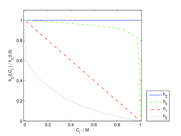
Figure 1: The relationships between the pool counting process $C_{t^{-}}/M$ and its intensity ratio $h_{C}(t;C_{t^{-}})/h_{C}(t;C_{t^{-}}=0)$ in the four different cases summarized in Section 3.4. The cluster intensities for the GPL and GPCL models are listed in the rightmost columns of the two panels of Table 5.

1. Repeated defaults. The counting process can increase without limit, as implictly done in Lindskog and McNeil (2003).

   $$C_{t}=Z_{t},\ \ h_{Z}(t)=h_{C}(t)=\sum_{j=1}^{M}j\,{M\choose j}\widetilde{\lambda}_{j}(t)$$

2. Strategy 0. The counting process is bounded by the mapping $\psi(\cdot):=\min(\cdot,M)$, as in Brigo, Pallavicini and Torresetti (2006a). This is the Generalized Poisson Loss (GPL) model.

   $$C_{t}=\min(Z_{t},M),\ \ h_{0}(t):=h_{C}(t)=\sum_{j=1}^{M}\min(j,(M-Z_{t^{-}})^{+}){M\choose j}\widetilde{\lambda}_{j}(t)$$

3. Strategy 1. The counting process is bounded by forcing each single name to jump at most once. A dynamics, leading to a similar form of the intensity, is considered also in Elouerkhaoui (2006).

   $$C_{t}={Z}^{1}_{t},\ \ h_{1}(t):=h_{C}(t)=\left(1-\frac{{Z}^{1}_{t^{-}}}{M}\right)\sum_{j=1}^{M}j\,{M\choose j}\widetilde{\lambda}_{j}(t)$$

4. Strategy 2. The counting process is bounded by forcing clusters dynamics to give raise to at most one jump in each single name. This is the Generalized Poisson Cluster Loss (GPCL) model.

   $$C_{t}=Z^{2}_{t},\ \ h_{2}(t):=h_{C}(t)=\sum_{j=1}^{M}j\,{M-Z^{2}_{t^{-}}\choose j}\widetilde{\lambda}_{j}(t)$$

In Figure 1 we plot $h_{C}(t;C_{t^{-}})/h_{C}(t;C_{t^{-}}=0)$ against $C_{t^{-}}/M$ in the four cases. The cluster intensities $\widetilde{\lambda}_{j}$ for the first and the third model are not relevant, since their influence cancels taking the ratio. The cluster intensities for the second and the fourth model are calibrated against the 10-year DJi-TRAXX tranche and index spreads on October 2, 2006 (see Table 5).

Notice, further, that for any choice of the cluster intensities the pool intensities are monotonic non-increasing functions of the pool counting process, not explicitly depending on time.

4 Beyond GPL: The GPCL model calibration

In Brigo, Pallavicini and Torresetti (2006a) the GPL basic model $C_{t}=\min(Z_{t},M)$ is calibrated to the index and its tranches for several maturities. Here we try instead the richer GPCL model $C_{t}=Z^{2}_{t}$ introduced above, allowing us in principle to model also cluster and single name defaults consistently. However, the GPCL model can hardly be managed without simplifying assumptions. In the following we assume again that the cluster intensities $\widetilde{\lambda}_{s}$ depend only on the cluster size $|s|$. Moreover, as with the basic GPL model, we try calibration of multi-name products only, such as credit indices and CDO tranches, leaving aside single name data for the time being. Indeed, with respect to our earlier paper in Brigo Pallavicini and Torresetti (2006a), we focus only on the improvement in calibration due to using a default counting process whose intensity has a clear interpretation in terms of default clusters. This will allow us, in further work, to include single names in the picture, since our GPCL framework allows us to do so explicitly.

The recovery rate is considered as a deterministic constant and set equal to $R=40\%$. Thus, the underlying driving model definition is

$$C_{t}:=Z^{2}(t)=\sum_{j=1}^{M}j\,Z^{2}_{j}(t),\ \ \mbox{where}\ \ \ dZ^{2}_{j}(t)\sim{\rm Poisson}\left({M-Z^{2}_{t^{-}}\choose j}\widetilde{\lambda}_{j}(t)dt\right)$$

while the pool counting and loss processes are defined as

$$d{\bar{C}}_{t} := dZ^{2}_{t}/M$$

$$d{\bar{L}}_{t} := (1-R)\,dZ^{2}_{t}/M$$

In the following sections we first discuss the numerical issues concerning calibration, and, then, we show some model calibration results.

4.1 Numerical issues concerning calibration

Given our recovery assumption, the prices of the products to be calibrated, presented in the appendix, depend only on knowledge of the probability distribution of the pool counting process $C_{t}$. Thus, our main issue is to calculate this law as fast as possible. When dealing with dynamics derived from Poisson processes, there are different available calculation methods, depending on the structure of the intensities.

If the intensity does not depend on the process itself, or it does only in a simple way, then the probability distribution can be derived by means of Fast Fourier inversion of the characteristic function, when the latter is available in closed form. This method is described and used for the GPL model in Brigo, Pallavicini and Torresetti (2006a,b). Again, the GPL process is based on the driver $Z$, that can be interpreted also as a compound Poisson process, as we have seen in Section 2.3. In general the probability distributions of compound Poisson processes can be calculated in closed form if the i.i.d. jump amplitudes have a discrete-valued distribution. Consider the compound Poisson process defined in Section 2.3. It is possible to find a relationship, known as Panjer recursion, between the probability densities $p_{X_{t}}(n)$ and $p_{X_{t}}(n-1)$ as done in Hess et al. (2002).

However, with the GPCL model, the dependence of the intensity of the pool counting process on the process itself prevents us either to calculate the relevant characteristic function in closed form or to use the Panjer method.

Our choice then is to explicitly calculate the forward Kolmogorov equation satisfied by the probability distribution $p_{Z^{2}_{t}}(x)=\mathbb{Q}\left\{\,Z^{2}_{t}=x\,\right\}$, namely

$$\frac{d}{dt}p_{Z^{2}_{t}}(x)=\sum_{y=0}^{M}A_{t}(x,y)p_{Z^{2}_{t}}(y)$$

where the transition rate matrix $A_{t}=(A_{t}(x,y))_{x,y=0,\ldots,M}$ is given by

$$A_{t}(x,y):=\lim_{\Delta t\rightarrow 0}\frac{\mathbb{Q}\left\{\,Z^{2}_{t+\Delta t}=x|Z^{2}_{t}=y\,\right\}}{\Delta t}={M-y\choose x-y}\widetilde{\lambda}_{x-y}(t)$$

for $x>y$,

$$A_{t}(y,y):=\lim_{\Delta t\rightarrow 0}\frac{\mathbb{Q}\left\{\,Z^{2}_{t+\Delta t}=y|Z^{2}_{t}=y\,\right\}-1}{\Delta t}=-\sum_{j=1}^{M-y}{M-y\choose j}\widetilde{\lambda}_{j}(t).$$

for $x=y$, and zero for $x<y$.

In matrix form we write

$$\frac{d}{dt}\widehat{\pi}_{t}=A_{t}\widehat{\pi}_{t},\ \ \ \ \ \widehat{\pi}_{t}:=\left[\begin{array}[]{ccccc}p_{Z^{2}_{t}}(0)&p_{Z^{2}_{t}}(1)&p_{Z^{2}_{t}}(2)&\ldots&p_{Z^{2}_{t}}(M)\end{array}\right]^{\prime}$$

whose solution is obtained through the exponential matrix,

$$\widehat{\pi}_{t}=\exp\left(\int_{0}^{t}A_{u}du\right)\widehat{\pi}_{0},\ \ \widehat{\pi}_{0}=[1\ 0\ 0...\ 0]^{\prime}.$$

Matrix exponentiation can be quickly computed with the Padé approximation (see Golub and Van Loan (1983)), leading to a closed form solution for the probability distribution $p_{C_{t}}=\widehat{\pi}_{t}$ of the pool counting process $C_{t}$. This distribution can then be used in the calibration procedure.

4.2 GPCL model detailed Calibration procedure

If we define the cumulated cluster intensities as

$$\widetilde{\Lambda}_{j}(t)=\int_{0}^{t}\widetilde{\lambda}_{j}(u)\,du.$$

then the entries of the matrix undergoing exponentiation in determining the default counting distribution are given by

$${\rm for~{}}x>y{\rm:~{}}\int_{0}^{t}A_{u}(x,y)du={M-y\choose x-y}\widetilde{\Lambda}_{x-y}(t)$$

$${\rm for~{}}x=y{\rm:~{}}\int_{0}^{t}A_{u}(y,y)du=-\sum_{j=1}^{M-y}{M-y\choose j}\widetilde{\Lambda}_{j}(t).$$

We assume the $\widetilde{\Lambda}_{j}$ to be piecewise linear in time, changing their values at payoff maturity dates. We use $\widetilde{\Lambda}_{j}$ as calibration parameters. We have $bM$ free calibration parameters, if we consider $b$ maturities. Notice that many $\widetilde{\Lambda}_{j}(t)$ will be equal to zero for all maturities, meaning that we can ignore their corresponding counting process $Z^{2}_{j}(t)$. One can think of deleting all the modes with jump sizes having zero intensity and keep only the nonzero intensity ones. Call $\alpha_{1}<\alpha_{2}<...<\alpha_{n}$ the jump sizes with nonzero intensity. Then one renumbers progressively the intensities according to the nonzero increasing $\alpha$: $Z^{2}_{j}$ becomes the jump of a cluster of size $\alpha_{j}$.

The calibration procedure for GPCL is implemented using the $\alpha_{j}$ in the same way as in Brigo, Pallavicini and Torresetti (2006a) for the GPL model. As concerns the GPCL intensities, in the tables we display ${M\choose\alpha_{j}}\widetilde{\Lambda}_{j}$, i.e. we multiply a cluster cumulated intensity for a given cluster size for the number of clusters with that size at time $0$.

We also calibrate the GPL model, for comparison. In this paper we denote the GPL cumulated intensities for the $\alpha_{j}$ mode by ${\Lambda}_{j}^{0}$, which reads, using the link with repeated defaults, as ${\Lambda}_{j}^{0}={M\choose\alpha_{j}}\widetilde{\Lambda}_{j}$. Given the arbitrary a-posteriori capping procedure in GPL, these $\widetilde{\Lambda}_{j}$ are not to be interpreted as cluster parameters, the only actual parameters being the ${\Lambda}_{j}^{0}$ directly, and they are to be interpreted as merely describing the pool counting process dynamic features.

More in detail, the optimal values for the amplitudes $\alpha_{j}$ in GPCL are selected, by adding non-zero amplitudes one by one, as follows, where typically $M=125$:

1. set $\alpha_{1}=1$ and calibrate $\widetilde{\Lambda}_{1}$;

2. add the amplitude $\alpha_{2}$ and find its best integer value by calibrating the cumulated intensities $\widetilde{\Lambda}_{1}$ and $\widetilde{\Lambda}_{2}$, starting from the previous value for $\widetilde{\Lambda}_{1}$ as a guess, for each value of $\alpha_{2}$ in the range $[1,125]$,

3. repeat the previous step for $\alpha_{i}$ with $i=3$ and so on, by calibrating the cumulated intensities $\widetilde{\Lambda}_{1},\dots,\widetilde{\Lambda}_{i}$, starting from the previously found $\widetilde{\Lambda}_{1},\dots,\widetilde{\Lambda}_{i-1}$ as initial guess, until the calibration error is under a pre-fixed threshold or until the intensity $\widetilde{\Lambda}_{i}$ can be considered negligible.

The objective function $f$ to be minimized in the calibration is the squared sum of the errors shown by the model to recover the tranche and index market quotes weighted by market bid-ask spreads:

$$f(\alpha,\widetilde{\Lambda})=\sum_{i}\epsilon_{i}^{2},\ \ \epsilon_{i}=\frac{x_{i}(\alpha,\widetilde{\Lambda})-x_{i}^{\rm Mid}}{x_{i}^{\rm Bid}-x_{i}^{\rm Ask}}$$ (18)

where the $x_{i}$, with $i$ running over the market quote set, are the index values $S_{0}$ for DJi-TRAXX index quotes, and either the index periodic premiums $S^{A,B}_{0}$ or the upfront premium rates $U^{A,B}$ for the DJi-TRAXX tranche quotes, see the appendix for more details.

4.3 Calibration results

The calibration data set is the DJi-TRAXX main series on the run on October, 2 2006. In Tables 2 and 3 we list the discount interest rates, the CDO tranche spreads and the credit index spreads.

We calibrate three methods against such data set and we compare the results. They are listed in the tables.

1. The implied expected tranched loss method (hereafter ITL) described in Walker (2006) or in Torresetti, Brigo and Pallavicini (2006). It is a method which allows to check if arbitrage opportunities are present on the market by implying expected tranched losses satisfying basic no-arbitrage requirements.

2. The GPL model described in Brigo, Pallavicini and Torresetti (2006a) and summarized above, i.e. $C_{t}=\min(Z_{t},M)$ with $Z$ as in (5) (referred to before as strategy 0). Such model, due to the capping feature, is not compatible with any of the previously described single-name dynamics avoiding repeated defaults.

3. The GPCL model described in the present paper (strategy 2), which represents an articulated solution to the repeated defaults problem. We implement the simplified version with cluster intensity $\widetilde{\lambda}_{s}$ depending only on cluster size $|s|$.

First, we check that there are no arbitrage opportunities on October, 2 2006, by calibrating the ITL method. The calibration is almost exact and in Table 7 we show the expected tranched losses implied by the method, which we can use as reference values when comparing the other two models.

Then we calibrate the GPL and GPCL models, and we obtain the calibration parameters presented in Table 5, while the expected tranched losses implied by these two models are included in Table 7. We point out that this is a joint calibration across tranche seniority and maturity, since we are calibrating all and every tranche and index quote with a single model specification. When looking at the outputs of the calibrated models on the different maturities, we see that both our models perform very well on maturities of 3 years, 5 years and 7 years, for which the calibration error is within the bid-ask spread. The 10 year maturity quotes are more difficult to recover, but both models are close to the market values, as we see from the left panel of Table 8. Notice, however, that the GPCL model has a lower calibration error ($10\%-20\%$ better).

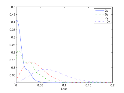
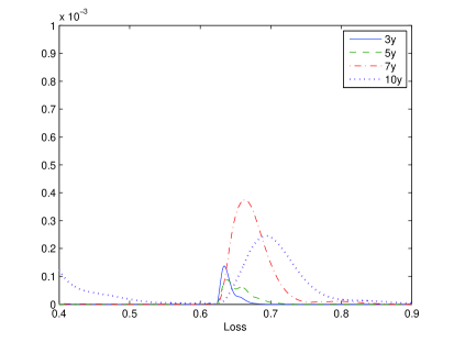
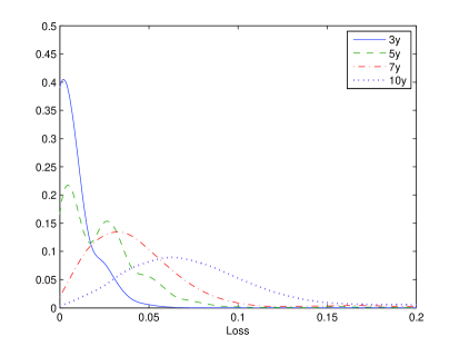
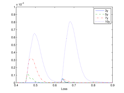
Figure 2: Loss distribution evolution of the GPL model (upper panel) and of the GPCL model (lower panel) at all the quoted maturities up to ten years, drawn as a continuous line.

The probability distributions implied by the two dynamical models are similar at gross-grain view, as one can see in Figure 2, but they differ if we observe the fine structure. Indeed, the tails of the two distributions show different bumps. The GPCL model shows a more complex pattern, and, as one can see from Table 5, its highest mode is the maximum portfolio loss, while the GPL model has a less clear tail configuration.

We also apply the ITL, GPL and GPCL methods to the CDX index and tranches (see Table 4 for market quotes), following the same procedure used for the DJi-TRAXX above. We find better results, that are summarized in Table 6 and in the right panel of Table 8.

5 Model Extensions

In this final section we hint at possible extensions of the basic model to account for more sophisticated features.

5.1 Spread dynamics

The valuation of credit index forward contracts or options maturing at time $T=T_{a}$ requires the calculation of the index spread at those future times, which in turn depends on the default intensity evolution. Consider, for instance, the case of deterministic interest rates (or more generally interest rates independent of defaults) for an index whose default leg protects against losses in the index pool up to time $T_{b}$ and where the spread premium payments occur at times $T_{1},T_{2},\ldots,T_{b}$. We have the spread expression at $T_{a}$ as

$$S_{T}=\frac{\int_{T}^{T_{b}}D(T,t)\,\mathbb{E}_{T}\!\left[\,h_{\bar{L}}(t)\,\right]dt}{\sum_{i=1}^{b}\,\delta_{i}D(T,T_{i})\left(1-{\bar{C}}_{T}-\int_{T}^{T_{i}}\mathbb{E}_{T}\!\left[\,h_{\bar{C}}(t)\,\right]dt\right)1_{\{T_{i}>T\}}}$$

where $h_{\bar{L}}(t)$ is the default intensity of the cumulated portfolio loss process and $h_{\bar{C}}(t)$ is the default intensity of the re-scaled default counting process ${\bar{C}}$ (see for example Brigo, Pallavicini e Torresetti (2006a), or the Appendix, for a detailed description of credit index contracts) and $D(s,t)$ is the discount factor, often assumed to be deterministic, between times $s$ and $t$.

The GPCL model presented in the previous sections has single-name and default counting intensities given by equations (16). These intensities depend on which names have already defaulted. The dynamics of the index $S_{t}$ (spread dynamics) can be enriched by more sophisticated modelling of the default intensities $h_{\bar{L}}(t)$ and $h_{\bar{C}}(t)$, by explicitly adding stochasticity to the Poisson intensities $\widetilde{\lambda}_{j}(t)$, e.g. resorting to the Gamma, scenario or CIR extensions of the model seen above.

5.2 Spread dynamics through Gamma intensity

Assume now that the cumulated clusters intensities $\widetilde{\Lambda}_{s}(t):=\int_{0}^{t}\,\widetilde{\lambda}_{s}(u)du$ are distributed at any time $t$ according a Gamma distribution, i.e.

$$\widetilde{\Lambda}_{s}(t)\sim\Gamma(k_{s}(t),\theta_{s})$$

where $k>0$ is the shape parameter and $\theta>0$ is the scale parameter in the Gamma distribution. These gamma processes are assumed to be independent of the exponential random variables triggering the jumps in the $\widetilde{N}_{s}$ Poisson processes. The Gamma choice is convenient because it does not alter the tractability of the basic model. See Brigo, Pallavicini e Torresetti (2006b) for a Gamma GPL implementation.

The Gamma distribution assumption for $\widetilde{\Lambda}_{s}(t)\sim\Gamma(k_{s}(t),\theta_{s})$ at every time $t$ is consistent with a Gamma process assumption for $\widetilde{\Lambda}_{s}(t)$, whose distribution is controlled by both parameters $k$ and $\theta$. The time constant $\theta$ allows for little flexibility in the variance term-structure of the process. In Brigo, Pallavicini and Torresetti (2006b) we improve the model in this respect, by introducing a piecewise Gamma GPL process extension.

5.3 Spread dynamics through CIR intensity

A different and possibly more interesting extension is to model the cluster intensities according to a Cox Ingersoll Ross (CIR) process

$$d\widetilde{\lambda}_{s}(t)=k_{s}(\theta_{s}-\widetilde{\lambda}_{s}(t))dt+\sigma_{s}\sqrt{\widetilde{\lambda}_{s}(t)}dW_{s}$$

with $2k_{s}\theta_{s}>\sigma_{s}^{2}$. These CIR processes are assumed to be independent of the exponential random variables triggering the jumps in the $\widetilde{N}_{s}$ Poisson processes.

With respect to the case of deterministic cluster intensities, the model tractability is preserved, due to the closed form results which can be derived. Alternatively, jump diffusion JCIR intensities can be considered, maintaining tractability.

5.4 Spread dynamics through Scenario intensity

A different extension is as follows. By taking scenarios on the clusters intensities we may easily extend our basic model. In this model we assume the intensities in all the clusters to take different scenarios with different probabilities. Indeed, assume now that the (possibly time varying) intensities $\widetilde{\lambda}_{s}$ are indexed by a random variable $I$ taking values $1,2,\ldots,m$ with (risk-neutral) probabilities $q_{1},q_{2},\ldots,q_{m}$: $\widetilde{\lambda}_{s}^{I}$ is then a random intensity for the $s$-th cluster process, depending on $I$. The related Poisson process is denoted by $\widetilde{N}_{s}^{I}$. $I$ is assumed to be independent of the exponential random variables triggering the jumps of the Poisson processes. Conditional on $I=i$, the intensity of the process $\widetilde{N}^{I}_{s}$ is $\widetilde{\lambda}_{s}^{i}$. This formulation does not spoil analytical tractability, since all the expected values can be calculated as a linear combination of conditional expectations.

5.5 Recovery dynamics

We introduced in (2), reported below here, the notion of recovery at default $R_{t}$:

$$d{\bar{L}}_{t}=(1-R_{t})d{\bar{C}}_{t}\ \ \ \ (\mbox{or, more precisely}\ \ \ {\bar{L}}_{t}=\int_{0}^{t}(1-R_{u})d{\bar{C}}_{u}).$$ (19)

Now we specify more about this notion. In general, for ease of computation, we assume $R_{t}$ to be a ${\cal G}_{t}$-adapted and left-continuous (and hence predictable) process taking values in the interval $[0,1]$. On predictability of the recovery process see also Bielecki and Rutkowski (2001). Here ${\cal G}_{t}$ denotes the filtration consisting of default-free market information and of the default-count monitoring up to time $t$. This implies in particular, given (19), that the loss ${\bar{L}}_{t}$ is ${\cal G}_{t}$-adapted too, as is reasonable. We noticed earlier that the no-arbitrage condition (1) is met if $R$ takes values in $[0,1]$. Equation (19) leaves us with the freedom of defining only two processes among ${\bar{L}}_{t}$, ${\bar{C}}_{t}$ and $R_{t}$. The more natural approach would be modeling explicitly $({\bar{C}}_{t},R_{t})$, obtaining ${\bar{L}}_{t}$, or modeling explicitly $({\bar{L}}_{t},R_{t})$, obtaining ${\bar{C}}_{t}$, all of them adapted.

However, if we choose to model both ${\bar{L}}_{t}$ and ${\bar{C}}_{t}$ as ${\cal G}_{t}$-adapted processes and to infer $R_{t}$, we have to ensure that the resulting process $R_{t}$ implicit in (19) is indeed left-continuous (and hence ${\cal G}_{t}$-predictable).

Indeed, in some formulations the predictability of the recovery is not possible. It is also a notion not always realistic: whether one or 125 names default in instant $(t-dt,t]$ (i.e. $dC_{t}=1$ or $dC_{t}=125$, respectively), we would be imposing the recovery $R_{t}$ to be the same in both cases and, in particular, to depend only on the information up to $t^{-}$.

However, under adapted-ness and left-continuity the recovery rate can be expressed also in terms of the intensities of the loss and default rate processes. From equation (19), by definition of compensator, we obtain

$$R_{t}=1-\frac{h_{\bar{L}}(t)}{h_{\bar{C}}(t)}.$$ (20)

Equation (20) shows that the recovery rate at default is directly related to the intensities of both the loss and the default rate processes. Thus, the choice for the intensity dynamics does induce a dynamics for the recovery rate.

In Brigo, Pallavicini and Torresetti (2006b) the cumulated portfolio loss process ${\bar{L}}$ is directly modelled as a GPL-type process with deterministic intensities and an extended set of allowed jump amplitudes that go beyond $1/M,2/M,\ldots,1$, according to (7). In this approach the recovery is implicitly defined. Numerical results show that calibrations are better with respect to the choice of modeling the default counting process as a GPL process instead (Brigo, Pallavicini, and Torresetti (2006a)). The direct loss modeling allows for both portfolio total loss and for more granular small-size losses. In particular super-senior tranches seem to be quoted taking into account the possibility of portfolio total loss, so that the direct loss model outperforms the default counting process model with a constant or simple recovery formulation.

On the other hand, the GPCL model derived within the CPS framework in the preceding sections requires direct modeling of the pool counting process. Thus, if the recovery rate $R$ is constant, the portfolio total loss is forbidden, since bounded to be not greater than $1-R$ on a unit portfolio notional.

We now examine possible ways to model the loss more realistically, starting from a GPL or GPCL model formulated in terms of default counting process. This amounts to implicitly model the recovery rate, since the number of defaults and the loss are linked by the recovery at default.

5.6 Recovery dynamics through Deterministic mapping

A first approach to implicitly model recovery rates consists in defining the cumulated portfolio loss ${\bar{L}}_{t}$ process as a deterministic function of the pool counting process ${\bar{C}}_{t}$ via a deterministic map, as previously done when dealing with repeated defaults exceeding the pool size, through the a-posteriori capping technique used in the basic GPL model (see Section 3.1). Generalizing that approach leads to the setting

$${\bar{L}}_{t}:=\psi({\bar{C}}_{t}),$$

where $\psi$ is a non-decreasing deterministic function with $\psi(0)=0$ and $\psi(1)\leq 1$. What does this imply in terms of recovery dynamics? We can easily write

$$d{\bar{L}}_{t}=\sum_{k=1}^{M}\left[\frac{\psi({\bar{C}}_{t^{-}}+k/M)-\psi({\bar{C}}_{t^{-}})}{k/M}\right]1_{\{d{\bar{C}}_{t}=k/M\}}d{\bar{C}}_{t}$$

which shows that the recovery at default in this case would not be predictable, depending explicitly from $dC_{t}$, except for very special $\psi$’s.

A generalization based on a random process transformation (rather than a deterministic function) of the counting process leading to an implicit dynamics of the recovery process is presented in the next section.

5.7 Recovery dynamics through Gamma mapping

Consider a stochastic process $u\mapsto\Psi_{u}$ in time $u$, ${\cal G}_{u}$-adapted and taking values in $[0,1]$, right-continuous with left limit, and independent of the default counting process ${\bar{C}}_{t}$, and use it to map the positive non-decreasing pool counting process ${\bar{C}}_{t}$ taking values in $[0,1]$ into the portfolio cumulated loss ${\bar{L}}_{t}$, sharing the same characteristics, i.e. define

$${\bar{L}}_{t}:=\Psi_{{\bar{C}}_{t}}.$$

Further, assume the process satisfies the following requirements, enforcing the no-arbitrage conditions:

$$\Psi_{0}=0,\quad\Psi_{1}\leq 1,\quad{\rm and}\quad d\Psi_{t}\geq 0$$

This way the cumulated portfolio loss can be viewed as a stochastic time change of the process $\Psi$. Further, in order to allow for portfolio total loss, we enforce the stronger condition

$$\Psi_{1}=1.$$

The time change does not spoil the analytical tractability of the model. If we know the probability distribution function of the pool counting process and of $\Psi$, we can simply derive the probability distribution function of the portfolio loss through an iterated expectation, thanks to independence:

$$\mathbb{Q}\left\{\,{\bar{L}}_{t}\leq x\,\right\}=\mathbb{E}\!\left[\,\mathbb{Q}\left\{\,{\bar{L}}_{t}\leq x|{\bar{C}}_{t}\,\right\}\,\right]=\int\mathbb{Q}\left\{\,\Psi_{y}\leq x\,\right\}p_{{\bar{C}}_{t}}(y)dy$$

As a relevant example, assume the process $u\mapsto\Psi_{u}$ is a Gamma process with shape parameter $\mu(u)$ and scale parameter $\nu$. The monotonicity of the resulting loss process can be easily checked, while the probability distribution of the process can be calculated explicitly. Indeed, as a direct calculation can show, for any times $s<t<T$, the conditional distribution of $\Psi_{t}$, given $\Psi_{s}$ and $\Psi_{T}$ is known in terms of the Beta distribution.

The calculation of the unconditional distribution of the cumulated portfolio loss follows directly.

Exactly as for the previous case based on the deterministic transform $\psi$, here the implicit recovery at default turns out to be not predictable in general.

6 Conclusions

We have extend the common Poisson shock (CPS) framework in two possible ways that avoid repeated defaults. The second way, more consistent with the original spirit of the CPS framework, leads to the Generalized-Poisson adjusted-Cluster-dynamics Loss model (GPCL) . We have illustrated the relationship of the GPCL with our earlier Generalized Poisson Loss (GPL) model, pointing out that while the GPCL model shares the good calibration power of the GPL model, it further allows for consistency with single names, thus constituing one of the few explict examples of top down approaches to loss modeling with real consistency for single names, or of bottom up approaches with real dynamical features.

Further research concerns recovery dynamics, calibration and analysis of forward start tranches and tranche options, when liquid quotes will be available, and analysis of calibration stability through history. A preliminary analysis of stability with the GPL model is however presented in Brigo, Pallavicini and Torresetti (2006b), showing good results. This is encouraging and leads to assuming the GPCL stability as well, although a rigorous check is in order in further work.

Appendix A Market quotes

The most liquid multi-name credit instruments available in the market are credit indices and CDO tranches (e.g. DJi-TRAXX, CDX).

A.1 Credit indices

The index is given by a pool of names $1,2,\ldots,M$, typically $M=125$, each with notional $1/M$ so that the total pool has unitary notional. The index default leg consists of protection payments corresponding to the defaulted names of the pool. Each time one or more names default the corresponding loss increment is paid to the protection buyer, until final maturity $T=T_{b}$ arrives or until all the names in the pool have defaulted.

In exchange for loss increase payments, a periodic premium with rate $S$ is paid from the protection buyer to the protection seller, until final maturity $T_{b}$. This premium is computed on a notional that decreases each time a name in the pool defaults, and decreases of an amount corresponding to the notional of that name (without taking out the recovery).

We denote with ${\bar{L}}_{t}$ the portfolio cumulated loss and with ${\bar{C}}_{t}$ the number of defaulted names up to time $t$ re-scaled by $M$. Thus, $0\leq{\bar{L}}_{t}\leq{\bar{C}}_{t}\leq 1$. The discounted payoff of the two legs of the index is given as follows:

$$\mbox{D{\tiny EF}L{\tiny EG}}(0):=\int_{0}^{T}D(0,t)d{\bar{L}}_{t}$$

$$\mbox{P{\tiny REMIUM}L{\tiny EG}}(0):=S_{0}\sum_{i=1}^{b}D(0,T_{i})\int_{T_{i-i}}^{T_{i}}(1-{\bar{C}}_{t})dt$$

where $D(s,t)$ is the (deterministic) discount factor between times $s$ and $t$. The integral on the right hand side of the premium leg is the outstanding notional on which the premium is computed for the index. Often the premium leg integral involved in the outstanding notional is approximated so as to obtain

$$\mbox{P{\tiny REMIUM}L{\tiny EG}}(0)=S_{0}\sum_{i=1}^{b}\,\delta_{i}D(0,T_{i})(1-{\bar{C}}_{T_{i}})$$

where $\delta_{i}=T_{i}-T_{i-1}$ is the year fraction.

Notice that, differently from what will happen with the tranches (see the following section), here the recovery is not considered when computing the outstanding notional, in that only the number of defaults matters.

The market quotes the value of $S_{0}$ that, for different maturities, balances the two legs. If one has a model for the loss and the number of defaults one may impose that the loss and number of defaults in the model, when plugged inside the two legs, lead to the same risk neutral expectation (and thus price) when the quoted $S_{0}$ is inside the premium leg, leading to

$$S_{0}=\frac{\mathbb{E}_{0}\!\left[\,\int_{0}^{T}D(0,t)d{\bar{L}}_{t}\,\right]}{\mathbb{E}_{0}\!\left[\,\sum_{i=1}^{b}\,\delta_{i}D(0,T_{i})(1-{\bar{C}}_{T_{i}})\,\right]}$$ (21)

A.2 CDO tranches

Synthetic CDO with maturity $T$ are contracts involving a protection buyer, a protection seller and an underlying pool of names. They are obtained by putting together a collection of Credit Default Swaps (CDS) with the same maturity on different names, $1,2,...,M$, typically $M=125$, each with notional $1/M$, and then “tranching” the loss of the resulting pool between the points $A$ and $B$, with $0\leq A<B\leq 1$.

$${\bar{L}}^{A,B}_{t}:=\frac{1}{B-A}\left[({\bar{L}}_{t}-A)1_{\{A<{\bar{L}}_{t}\leq B\}}+(B-A)1_{\{{\bar{L}}_{t}>B\}}\right]$$

Once enough names have defaulted and the loss has reached $A$, the count starts. Each time the loss increases the corresponding loss change re-scaled by the tranche thickness $B-A$ is paid to the protection buyer, until maturity arrives or until the total pool loss exceeds $B$, in which case the payments stop.

The discounted default leg payoff can then be written as

$$\mbox{D{\tiny EF}L{\tiny EG}}(0;A,B):=\int_{0}^{T}D(0,t)d{\bar{L}}^{A,B}_{t}$$

Again, one should not be confused by the integral, the loss ${\bar{L}}^{A,B}_{t}$ changes with discrete jumps. Analogously, also the total loss ${\bar{L}}_{t}$ and the tranche outstanding notional change with discrete jumps.

As usual, in exchange for the protection payments, a premium rate $S^{A,B}_{0}$, fixed at time $T_{0}=0$, is paid periodically, say at times $T_{1},T_{2},\ldots,T_{b}=T$. Part of the premium can be paid at time $T_{0}=0$ as an upfront $U^{A,B}_{0}$. The rate is paid on the “survived” average tranche notional. If we assume that the payments are made on the notional remaining at each payment date $T_{i}$, rather than on the average in $[T_{i-1},T_{i}]$, the discounted payoff of the premium leg can be written as

$$\mbox{P{\tiny REMIUM}L{\tiny EG}}(0;A,B):=U^{A,B}_{0}+S^{A,B}_{0}\sum_{i=1}^{b}\,\delta_{i}D(0,T_{i})(1-{\bar{L}}^{A,B}_{T_{i}})$$

where $\delta_{i}=T_{i}-T_{i-1}$ is the year fraction.

When pricing CDO tranches, one is interested in the premium rate $S^{A,B}_{0}$ that sets to zero the risk neutral price of the tranche. The tranche value is computed taking the (risk-neutral) expectation (in $t=0$) of the discounted payoff consisting on the difference between the default and premium legs above. We obtain

$$S^{A,B}_{0}=\frac{\mathbb{E}_{0}\!\left[\,\int_{0}^{T}D(0,t)d{\bar{L}}^{A,B}_{t}\,\right]-U^{A,B}_{0}}{\mathbb{E}_{0}\!\left[\,\sum_{i=1}^{b}\,\delta_{i}D(0,T_{i})(1-{\bar{L}}^{A,B}_{T_{i}})\,\right]}$$ (22)

The above expression can be easily recast in terms of the upfront premium $U^{A,B}_{0}$ for tranches that are quoted in terms of upfront fees.

The tranches that are quoted on the market refer to standardized pools, standardized attachment-detachment points $A-B$ and standardized maturities $T$.

Actually, for the i-Traxx and CDX pools, the equity tranche $(A=0,B=3\%)$ is quoted by means of the fair $U^{A,B}_{0}$, while assuming $S^{A,B}_{0}=500bps$. All other tranches are quoted by means of the fair $S^{A,B}_{0}$, assuming no upfront fee ($U^{A,B}_{0}=0)$.

Appendix B Tables: Calibration Inputs and Outputs

Date	Rate	Date	Rate	Date	Rate	Date	Rate
20-Dec-06	3.41%	21-Sep-09	3.71%	20-Jun-12	3.75%	20-Mar-15	3.83%
20-Mar-07	3.57%	21-Dec-09	3.72%	20-Sep-12	3.76%	22-Jun-15	3.84%
20-Jun-07	3.66%	22-Mar-10	3.72%	20-Dec-12	3.76%	21-Sep-15	3.84%
20-Sep-07	3.70%	21-Jun-10	3.72%	20-Mar-13	3.77%	21-Dec-15	3.85%
20-Dec-07	3.72%	20-Sep-10	3.72%	20-Jun-13	3.77%	21-Mar-16	3.86%
20-Mar-08	3.72%	20-Dec-10	3.72%	20-Sep-13	3.78%	20-Jun-16	3.87%
20-Jun-08	3.72%	21-Mar-11	3.73%	20-Dec-13	3.79%	20-Sep-16	3.87%
22-Sep-08	3.72%	20-Jun-11	3.73%	20-Mar-14	3.80%	20-Dec-16	3.88%
22-Dec-08	3.72%	20-Sep-11	3.74%	20-Jun-14	3.80%
20-Mar-09	3.71%	20-Dec-11	3.74%	22-Sep-14	3.81%
22-Jun-09	3.71%	20-Mar-12	3.74%	22-Dec-14	3.82%

Table 2: EUR zero-coupon continuously-compounded spot rates (ACT/365).

	Att-Det	Maturities
		3y	5y	7y	10y
Index		18(0.5)	30(0.5)	40(0.5)	51(0.5)
Tranche	0-3	350(150)	1975(25)	3712(25)	4975(25)
	3-6	5.50(4.0)	75.00(1.0)	189.00(2.0)	474.00(4.0)
	6-9	2.25(3.0)	22.25(1.0)	54.25(1.5)	125.50(3.0)
	9-12		10.50(1.0)	26.75(1.5)	56.50(2.0)
	12-22		4.00(0.5)	9.00(1.0)	19.50(1.0)
	22-100		1.50(0.5)	2.85(0.5)	3.95(0.5)

Table 3: DJi-TRAXX index and tranche quotes in basis points on October 2, 2006, along with the bid-ask spreads. Index and tranches are quoted through the periodic premium, whereas the equity tranche is quoted as an upfront premium. See Appendix A.

	Att-Det	Maturities
		3y	5y	7y	10y
Index		24(0.5)	40(0.5)	49(0.5)	61(0.5)
Tranche	0-3	975(200)	3050(100)	4563(200)	5500(100)
	3-7	7.90(1.6)	102.00(6.1)	240.00(48.0)	535.00(21.4)
	7-10	1.20(0.2)	22.50(1.4)	53.00(10.6)	123.00(7.4)
	10-15	0.50(0.1)	10.25(0.6)	23.00(4.6)	59.00(3.5)
	15-30	0.20(0.1)	5.00(0.3)	7.20(1.4)	15.50(0.9)

Table 4: CDX index and tranche quotes in basis points on October 2, 2006, along with the bid-ask spreads. Index and tranches are quoted through the periodic premium, whereas the equity tranche is quoted as an upfront premium. See Appendix A.

$\alpha_{j}$	${\Lambda}^{0}_{j}(T)$
	3y	5y	7y	10y
1	0.778	1.318	3.320	4.261
3	0.128	0.536	0.581	1.566
15	0.000	0.004	0.024	0.024
19	0.000	0.007	0.011	0.028
32	0.000	0.000	0.000	0.007
79	0.000	0.000	0.003	0.003
120	0.000	0.002	0.003	0.008

$\alpha_{j}$	${M\choose\alpha_{j}}{\widetilde{\Lambda}}_{j}(T)$
	3y	5y	7y	10y
1	0.882	1.234	3.223	3.661
3	0.128	0.615	0.682	1.963
15	0.001	0.002	0.023	0.023
19	0.000	0.009	0.016	0.043
57	0.000	0.000	0.002	0.007
80	0.000	0.000	0.000	0.010
125	0.001	0.005	0.042	0.042

Table 5: DJi-TRAXX pool. Left side: cumulated intensities, integrated up to tranche maturities, of the basic GPL model. Each row $j$ corresponds to a different Poisson component with jump amplitude $\alpha_{j}$. Right side: cumulated cluster intensities, integrated up to tranche maturities, and multiplied by the number of clusters of the same size at time $0$. Each row $j$ corresponds to a different cluster size $\alpha_{j}$. The amplitudes/cluster-sizes not listed have an intensity below $10^{-7}$. The recovery rate is $40\%$.

$\alpha_{j}$	${\Lambda}^{0}_{j}(T)$
	3y	5y	7y	10y
1	1.132	3.043	4.247	7.166
2	0.189	0.189	0.812	1.625
6	0.011	0.091	0.091	0.091
18	0.000	0.006	0.028	0.028
23	0.000	0.004	0.005	0.032
32	0.000	0.000	0.000	0.009
124	0.000	0.003	0.005	0.010

$\alpha_{j}$	${M\choose\alpha_{j}}\widetilde{\Lambda}_{j}(T)$
	3y	5y	7y	10y
1	0.063	0.552	3.100	6.661
2	0.804	1.531	1.531	2.076
3	0.020	0.195	0.195	0.195
17	0.000	0.010	0.037	0.087
32	0.000	0.003	0.009	0.032
110	0.000	0.000	0.000	0.010
125	0.000	0.011	0.054	0.054

Table 6: CDX pool. Left side: cumulated intensities, integrated up to tranche maturities, of the basic GPL model. Each row $j$ corresponds to a different Poisson component with jump amplitude $\alpha_{j}$. Right side: cumulated cluster intensities, integrated up to tranche maturities, and multiplied by the number of clusters of the same size at time $0$. Each row $j$ corresponds to a different cluster size $\alpha_{j}$. The amplitudes/cluster-sizes not listed have an intensity below $10^{-7}$. The recovery rate is $40\%$.

		Tranches
Models	Maturities	0-3	3-6	6-9	9-12	12-22	22-100
ITL	3y	18.6%	0.2%	0.1%	0.0%	0.0%	0.0%
	5y	44.6%	4.2%	1.2%	0.6%	0.2%	0.1%
	7y	71.0%	14.5%	4.3%	2.1%	0.7%	0.2%
	10y	91.6%	49.2%	14.1%	6.4%	2.2%	0.4%
GPL	3y	18.6%	0.2%	0.1%	0.1%	0.0%	0.0%
	5y	44.5%	4.2%	1.2%	0.6%	0.2%	0.1%
	7y	70.8%	14.6%	4.3%	2.1%	0.7%	0.2%
	10y	91.2%	47.2%	14.6%	6.4%	2.2%	0.4%
GPCL	3y	18.7%	0.2%	0.1%	0.0%	0.0%	0.0%
	5y	44.7%	4.2%	1.2%	0.6%	0.2%	0.1%
	7y	70.9%	14.6%	4.3%	2.1%	0.7%	0.2%
	10y	91.2%	47.5%	14.5%	6.4%	2.2%	0.4%

Table 7: Implied expected tranched loss for the ITL, GPL and GPCL models. Results refer to DJi-TRAXX market.

	Att-Det	DJi-TRAXX 10y
		GPL	GPCL
Index		0.00	0.00
Tranche	0-3	0.76	0.62
	3-6	-2.35	-1.93
	6-9	1.21	1.04
	9-12	-0.40	-0.36
	12-22	0.02	0.02
	22-100	0.00	0.00

	Att-Det	CDX 10y
		GPL	GPCL
Index		0.00	-0.06
Tranche	0-3	1.43	1.60
	3-7	-0.45	-0.22
	7-10	0.22	0.25
	10-15	-0.08	-0.12
	15-30	0.01	0.07

Table 8: Calibration errors calculated with the GPL and GPCL models with respect to the bid-ask spread (i.e. $\epsilon_{i}$ in (18)) for tranches quoted by the market for the ten year maturity (see Tables 3 and 4). The left panel refers to DJi-TRAXX market quotes, while the right panel refers to CDX market quotes. Calibration errors for the other maturities are within the bid-ask spread and therefore they are not reported. The recovery rate is $40\%$ .

References

-
[1]
Balakrishna, B.S. (2006). A Semi-Analytical
Parametric Model for Credit Defaults.
Working paper, available at http://www.defaultrisk.com/pp_crdrv128.htm -
[2]
Bennani, N. (2005). The forward loss model: a dynamic
term structure approach for the pricing of portfolio credit derivatives.
Working paper available at http://defaultrisk.com/pp_crdrv_95.htm -
[3]
Bennani, N. (2006). A Note on Markov Functional
Loss Models.
Working Paper, available at http://www.defaultrisk.com/pp_cdo_01.htm - [4] Bielecki, T., and Rutkowski, M. (2001). Credit Risk: Modeling, Valuation and Hedging. Springer Verlag, Heidelberg.
- [5] Bielecki, T., Vidozzi, A., and Vidozzi, L. (2006). Pricing and hedging of basket default swaps and related derivatives. Preprint
-
[6]
Brigo, D., Pallavicini, A. and Torresetti, R. (2006a).
The Dynamical Generalized-Poisson loss model, Part one. Introduction and CDO calibration.
Short version to appear in Risk Magazine. Extended version available at
http://www.defaultrisk.com/pp_crdrv117.htm -
[7]
Brigo, D., Pallavicini, A. and Torresetti, R. (2006b).
The Dynamical Generalized-Poisson Loss model, Part two. Calibration stability and spread dynamics extensions.
Short version to appear in Risk Magazine. Extended version available at
http://www.defaultrisk.com/pp_crdrv117.htm - [8] Chapovsky, A., Rennie, A., and Tavares, P.A.C. (2006). Stochastic Intensity Modelling for Structured Credit Exotics. Merrill Lynch working paper.
-
[9]
Di Graziano, G., and Rogers, C. (2005), A new approach to the
modeling and pricing of correlation credit derivatives.
Working paper available at www.statslab.cam.ac.uk/chris/papers/cdo21.pdf - [10] Elouerkhaoui, Y. (2006). Pricing and Hedging in a Dynamic Credit Model, Citigroup Working paper, Presented at the conference “Credit Correlation: Life After Copulas”, London, Sept 29, 2006
-
[11]
Errais, E., Giesecke, K., and Goldberg, L. (2006).
Pricing credit from the top down with affine point processes.
Working paper available at
http://www.stanford.edu/dept/MSandE/people/faculty/giesecke/indexes.pdf -
[12]
Giesecke, K., and Goldberg, L. (2005). A top
down approach to multi-name credit.
Working paper available at
http://www.stanford.edu/dept/MSandE/people/faculty/giesecke/topdown.pdf - [13] Golub, H. and Van Loan, C. (1983). Matrix Computation, p. 384, Johns Hopkins University Press.
-
[14]
Hess, K., Liewald, A., Schmidt, K. (2002). An extension of Panjer’s recursion.
Astin Bulletin 32, 283-297. -
[15]
Lindskog, F., and McNeil, A. (2003).
Common Poisson shock models: applications to insurance and credit risk modelling.
Astin Bulletin 33, 209-238. -
[16]
Schönbucher, P. (2005). Portfolio losses and the term
structure of loss transition rates: a new methodology for the
pricing of portfolio credit derivatives.
Working paper available at http://defaultrisk.com/pp_model_74.htm -
[17]
Sidenius, J., Piterbarg, V., Andersen, L. (2005). A new framework
for dynamic credit portfolio loss modeling.
Working paper available at http://defaultrisk.com/pp_model_83.htm -
[18]
Torresetti, R., Brigo, D., and Pallavicini, A. (2006).
Implied Expected Tranched Loss Surface from CDO Data.
Working paper. -
[19]
Walker, M. (2006).
CDO models. Towards the next generation: incomplete markets and term structure.
Working paper available at http://defaultrisk.com/pp_crdrv109.htm