A Limit on the Polarized Anomalous Microwave Emission of Lynds 1622

Abstract

The dark cloud Lynds 1622 is one of a few specific sites in the Galaxy where, relative to observed free-free and vibrational dust emission, there is a clear excess of microwave emission. In order to constrain models for this microwave emission, and to better establish the contribution which it might make to ongoing and near-future microwave background polarization experiments, we have used the Green Bank Telescope to search for linear polarization at $9.65$ Ghz towards Lynds 1622. We place a $95.4\%$ upper limit of $88\,{\rm\mu K}$ ($123\,{\rm\mu K}$ at $99.7\%$ confidence) on the total linear polarization of this source averaged over a $1^{\prime}.3$ FWHM beam. Relative to the observed level of anomalous emission in Stokes I these limits correspond to fractional linear polarizations of $2.7\%$ and $3.5\%$.

1 Introduction

The discovery of anomalous dust-correlated emission by multi-frequency Microwave Background experiments in the 1990s (Leitch et al., 1997; de Oliveira-Costa et al., 1997; Kogut et al., 1996) led to a recalculation by Draine & Lazarian (1998a) of the electric dipole emission from small rotating dust grains, first considered by Erickson (1957). The emission is spatially correlated with dust, but far in excess of a reasonable extrapolation of the thermal emission (Finkbeiner et al., 1999) and is therefore called “anomalous” dust emission, or “Foreground X” (de Oliveira-Costa et al., 2002) because of its interference with cosmic microwave background (CMB) experiments. Since the Draine & Lazarian (1998a) paper on spinning dust, and a later paper proposing magnetic dipole emission from Fe containing grains (Draine & Lazarian, 1999) measurements of this component have been refined (e.g. de Oliveira-Costa et al., 1998; Finkbeiner et al., 2002; Banday et al., 2003; de Oliveira-Costa et al., 2004; Finkbeiner et al., 2004; Davies et al., 2006) using various data sets.

One yet untested prediction of the spinning dust theory is that the emission should be moderately polarized ($3-7\%$) at low frequencies, falling to under 2% above 20 GHz (Lazarian & Draine, 2000). At 10 GHz 3-5% linear polarization is expected. In contrast magnetic dipole fluctuations in larger single-domain grains would show a strong linear polarization ($\sim 10\%$) below 10 GHz, rising to over 30% at 100 GHz (Draine & Lazarian, 1999), although the details depend on the shape, iron fraction, and magnetic domain configuration of the grains. Because the polarization properties of the anomalous dust emission are unknown and are of immense interest to the CMB community, a deep exposure on a cloud known to contain the anomalous emission would make a substantial contribution to our understanding of this component.

Although anomalous, dust-correlated microwave emission has been detected statistically by numerous experiments, at the time of writing the number of individual lines of sight on which it is seen are but three: the NCP loop (Leitch et al., 1997); Lynds 1622 (Finkbeiner et al., 2002; Casassus et al., 2004); and Perseus (Watson et al., 2005). Battistelli et al. (2006) report the only measurement of the polarization of the anomalous emission, a detection of 3% fractional polarization in the Perseus cloud with the COSMOSOMAS experiment. We have used the GBT at $9\,{\rm GHz}$ to search for polarization towards Lynds 1622 (L1622).

2 Observations & Calibration

We chose to search for polarized emission from L1622 along the line of sight 05:54:23, $+01$:46:54 (J2000); this is the same pointing position used by Finkbeiner et al. in previous 9 GHz measurements of L1622. It is also near the peak of 30 GHz excess emission observed by CBI (Casassus et al., 2006). We observe at $9\,{\rm GHz}$, a frequency where the product of fractional linear polarization and total intensity for spinning dust is expected to be detectable (a few mK). This is also the lowest frequency GBT receiver equipped with circularly polarized feeds, which are essential to obtaining the broadband continuum stability needed for the Stokes Q and U measurements. Two sub-bands were chosen by examining site RFI monitor data, each of 200 MHz total bandwidth, centered on $8.65$ and $9.65$ GHz, respectively. Much wider bandwidth measurements are in principle possible, but RFI was a key consideration. The receiver temperature is smooth and low in these regions and avoid known spectral resonances.

The GBT X-band receiver has a single, dual-circularly polarized feed horn. The GBT Spectrometer was used to form all four auto- and cross-correlations between the IF signals from each of LCP and RCP, providing in principle instantaneous measurements of all four Stokes parameters ($I,Q,U,V$). The Stokes parameters describing linear polarization $(Q,U)$ principally comprise combinations of the cross-correlations, which has the advantage that receiver gain fluctuations and atmospheric emission variations are suppressed.

Successive pairs of On/Off measurements on L1622 were performed, each lasting 48 seconds and consisting of 1-second integrations. The On/Off pairs were matched in hour angle to provide approximately the same track in azimuth and elevation for each pair; allowing for scan-related observing overheads we found we required a separation of $\sim 66$ seconds in Right Ascension. This strategy minimizes the potential effect of polarized ground spillover, which would be expected to have a signature that changes with azimuth and elevation. Note however that the expected level of spillover is low due to the clear aperture, off-axis design of the GBT; deep integrations with the GBT $26-40\,{\rm GHz}$ receiver show that the level of any systematic signal in total intensity is $<100\,\,{\rm\mu Jy}$. The choice of trailing field was constrained by a compromise between observing efficiency and the benefits of short cycle times, particularly for the total intensity measurement. The timing accuracy of the GBT control system was not sufficient to allow an analogous LEAD region. In all  700 On/Off pairs were collected in 30 hours of observing. Every hour the telescope pointing and focus is checked on the nearby calibrator 3C138. 3C138 is also a well-measured polarization calibrator and we perform an On/Off measurement of 3C138 with the system configured identically to our L1622 polarization observations.

Prior to any calibration the data are flagged for RFI. Several fixed frequency ranges show common interfence events and are flagged in all scans ($9.57579-9.5777$ GHz; $9.6673-9.6688$ GHz; $9.7005-9.7018$ GHz; and any data over $9.730$ GHz). Beyond this the RL and LR data for each IF are searched and integration with a $>5\sigma$ spectral feature is flagged for rejection.

The full-Stokes data were calibrated using a variation on the procedures described in Heiles (2001); Heiles et al. (2001b, a), which we briefly review. A single noise diode is used to inject noise into each of LCP and RCP, and this (coherent) signal is used to determine the phase difference between the two IF paths. The dominant contributor to the R/L phase is the path length difference between the signal chains ($\sim 70\,{\rm cm}$). The response of the instrument to celestial polarization is described by the Mueller matrix (MM). We determine the MM from the 3C138 measurements assuming a fractional linear polarization of $11\%$ and a parallactic angle of $170^{\circ}$ of the linear polarization pseudovector. The data are also amplitude-calibrated using 3C138, for which we assume flux densities $S_{8.65}=2.43\,{\rm Jy}$ and $S_{9.65}=2.20\,{\rm Jy}$. This allows the determination of an effective Stokes I flux density of the calibration diode, $S_{cal}$, as a function of frequency across our observing band. After correcting for the measured LR phase difference and calibrating data for the bandpass as a function of frequency from the $S_{cal}$ data, means across the band are taken to form nominal Stokes $(I,Q,U,V)$ measurements. Mueller Matrices are computed from these data on the calibrator, and applied to the equivalent data on L1622. The result of these procedures is a position-switched Stokes $(I,Q,U,V)$ in Janskys per beam for each of 720 ON-OFF measurements of L1622 in our dataset. This is converted into a main-beam filling equivalent surface brightness by multiplying by the GBT gain (taken to be $1.95\,{\rm K/Jy}$ at $9.65{\,\rm GHz}$) and dividing by the main beam efficiency ($\eta_{B}\equiv\Omega_{mb}/\Omega_{ant}=93\%$).

The beam properties were determined by scans along six evenly spaced directions through 3C286, and orthogonal (az/el) scans through 3C138. We adopt a beam width of $1^{\prime}.30\,({\rm FWHM})$.

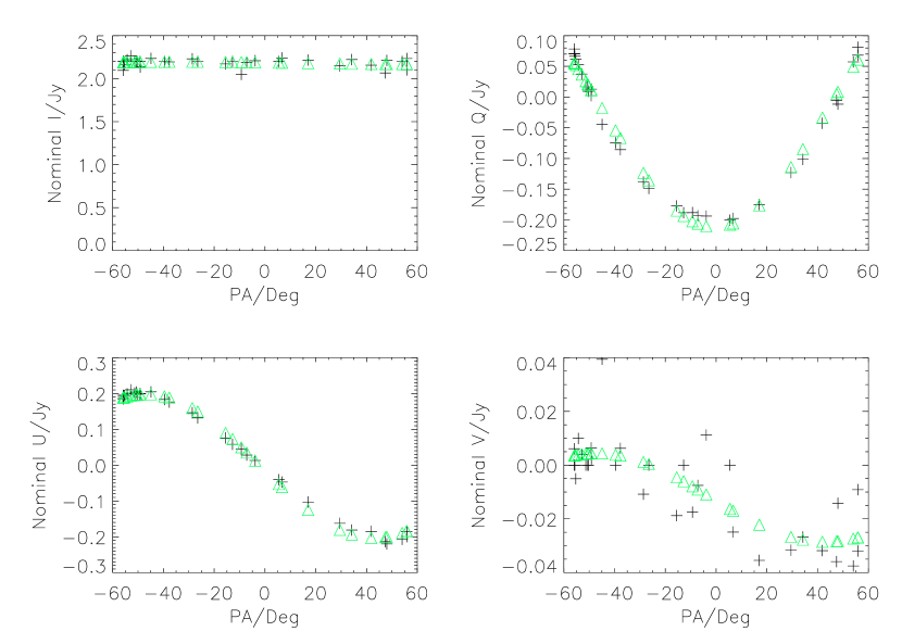
Figure 1: Measurements of 3C138 (black pluses) and the fitted Mueller Matrix describing the GBT polarization response (green triangles). The quantities shown are, from top left, the average autocorrelation (LL+RR); the real part of the LR cross correlation; the imaginary part of the LR cross correlation; the the difference between the autocorrelations.

The noise level was estimated from the data for each measurement by a robust, iterative procedure. First the the median absolute deviation of the measurements is computed for a given IF and Stokes parameter in a 3-hour buffer centered on the time of the measurement. We refer to the scatter so computed in this first pass on the data as $\sigma_{1}$. Data more than $6\sigma_{1}$ from the mean are rejected iteratively, i.e., if a data point(s) over the threshold exists, the worst outlier is rejected, the $\sigma$ recomputed, and the process repeated until there are no data over the threshold. This rejects $\sim 2\%$ of the data. After this process is completed the noises are recomputed using the variance in a sliding 3-hour buffer, resulting in a noise estimate $\sigma_{2}$ on the outlier-rejected data. Data with $\sigma_{2}$ values more than 5 times the expected radiometer noise ($S_{max,QU}=5\times 0.2\,\,{\rm mJy}$) in $Q$ and $U$ are rejected. Stokes $I$ data with noises more than $5$ times the best RMS ($S_{max,I}=5\times 10\,{\rm mJy}$) are rejected. This removes data collected in periods of less than optimal weather. Final results are computed as the weighted mean of individual measurements, with weights of $\sigma^{-2}_{2}$. The final results for each polarization are shown in Table 2 along with the average noise levels. Results for the $8.65$ GHz channel are consistent with those from the $9.65$ GHz channel but the Stokes $Q$ and $U$ parameters show noise levels a factor of $\sim 2$ higher, perhaps reflecting a hardware instability in these channels; we exclude them from our final results. The large variation in noise levels between the Stokes $I$, $Q$, $U$, and $V$ results is explained by the fact that with our observing technique both Stokes $I$ and $V$ are affected by receiver gain fluctuations, and Stokes $I$ is additionally affected by fluctuations in atmospheric emission, whereas Stokes $Q$ and $U$ largely are not.

A histogram of the individual measurements, normalized by the $\sigma_{2}$ value for each measurement is shown in Figure 2 along with the best-fit Gaussian to the distribution which should have a Gaussian $\sigma$ close to unity if our noise estimate is accurate. For Stokes $Q$ and $U$ the fitted Gaussians are within $5\%$ of unity; for $I$ and $V$, within $12\%$ of unity. While the data on the whole are well-described by a Gaussian distribution there are a small number of outliers. To determine the sensitivity of our results to these outliers, and to the noise estimate that results from our pipeline, we have varied our data filtering parameters in a suite of tests summarized in Table 1. The controlling parameters of our filtering procedure were systematically varied; the fully-averaged $9.65$ GHz Stokes parameters that result for each variation are shown in Figure 3. Note that our adopted parameters are denoted as “Test 0”.

The data binned by time and Parallactic Angle (PA) are shown in Figures 4 and 5, respectively. The overall consistency of the data are good, with the most significant deviation in Stokes $V$. The absence of significant variations in Stokes I, Q, and U with PA indicates that any residual ground signal is lower than the sensitivity achieved.

Figure 2: The distribution of individual measurements divided by their noise estimates ($8.65$ GHz is black and $9.65$ GHz is magenta). The dashed lines show the best-fitting Gaussian to each distribution. In all cases the Gaussian has a $\sigma$ within $4\%$ of unity indicating the accuracy of our noise estimate.

Figure 3: Fully averaged Stokes $I$, $Q$, $U$, and $V$ results for a range of filtering parameters. The dashed line shows our adopted value (test 0).

Figure 4: Mean values for each of Stokes $I$,$Q$,$U$, and $V$ with data binned in time over the course of the observing run.

Figure 5: Mean values for each of Stokes $I$,$Q$,$U$, and $V$ with data binned in parallactic angle.

Joint $1\sigma$, $2\sigma$, and $3\sigma$ confidence intervals on the $9.65$ GHz linear polarization signal are shown in Figure 6. These represent the difference in Stokes $Q$ and $U$ between the ON and OFF source locations, and on the assumption that the background signal is unpolarized at our observing frequency are limits on the polarization on the line of sight to L1622.

We note that there is a negative signal in Stokes $I$ on the line of sight to L1622. This is a robust result, likely due to small-scale variations in the free-free signal in the region; we discuss this possibility further in § 3.1.

Test	Buffer 1	Buffer 1 Reject	Buffer 2	Buffer 2 Reject	$Q,U$ Max.	$I$ Max.
Number	Scatter	Threshold	Scatter	Threshold	Buffer Noise	Buffer Noise
	Method	($S_{cut,1}$)	Method	($S_{cut,2}$)	($\sigma_{max,QU}$)	($\sigma_{max,I}$)
0	MAD	$6\sigma_{1}$	SD	No Rejection	1 mJy	50 mJy
1	MAD	$6\sigma_{1}$	SD	$4\sigma_{2}$	1 mJy	50 mJy
2	MAD	$6\sigma_{1}$	SD	$3\sigma_{2}$	1 mJy	50 mJy
3	MAD	$6\sigma_{1}$	MAD	No Rejection	1 mJy	50 mJy
4	MAD	$6\sigma_{1}$	MAD	$4\sigma_{2}$	1 mJy	50 mJy
5	MAD	$6\sigma_{1}$	MAD	$3\sigma_{2}$	1 mJy	50 mJy
6	MAD	$6\sigma_{1}$	SD	No Rejection	2 mJy	50 mJy
7	MAD	$6\sigma_{1}$	SD	$4\sigma_{2}$	2 mJy	50 mJy
8	MAD	$6\sigma_{1}$	SD	$3\sigma_{2}$	2 mJy	50 mJy
9	MAD	$6\sigma_{1}$	MAD	No Rejection	2 mJy	50 mJy
10	MAD	$6\sigma_{1}$	MAD	$4\sigma_{2}$	2 mJy	50 mJy
11	MAD	$6\sigma_{1}$	MAD	$3\sigma_{2}$	2 mJy	50 mJy
12	MAD	$6\sigma_{1}$	SD	No Rejection	$0.5$ mJy	50 mJy
13	MAD	$6\sigma_{1}$	SD	$4\sigma_{2}$	$0.5$ mJy	50 mJy
14	MAD	$6\sigma_{1}$	SD	$3\sigma_{2}$	$0.5$ mJy	50 mJy
15	MAD	$6\sigma_{1}$	MAD	No Rejection	$0.5$ mJy	50 mJy
16	MAD	$6\sigma_{1}$	MAD	$4\sigma_{2}$	$0.5$ mJy	50 mJy
17	MAD	$6\sigma_{1}$	MAD	$3\sigma_{2}$	$0.5$ mJy	50 mJy
18	MAD	$6\sigma_{1}$	SD	No Rejection	1 mJy	25 mJy
19	MAD	$6\sigma_{1}$	SD	No Rejection	1 mJy	25 mJy
20	MAD	$6\sigma_{1}$	SD	No Rejection	1 mJy	25 mJy
21	MAD	$6\sigma_{1}$	SD	No Rejection	1 mJy	100 mJy
22	MAD	$6\sigma_{1}$	SD	No Rejection	1 mJy	100 mJy
23	MAD	$6\sigma_{1}$	SD	No Rejection	1 mJy	100 mJy
24	SD	$6\sigma_{1}$	SD	No Rejection	1 mJy	50 mJy
25	N/A	No Rejection	SD	No Rejection	1 mJy	50 mJy
26	MAD	$3\sigma_{1}$	SD	No Rejection	1 mJy	50 mJy

Table 1: Data filter tests.

	Average ON-OFF	Typical Per-Measurement Noise
$I$	$-5.1\pm 1.4\,{\rm mK}$	$42\,{\rm mK}$
$Q$	$35\pm 30.\,{\rm\mu K}$	$0.81\,{\rm mK}$
$U$	$26\pm 34\,{\rm\mu K}$	$0.93\,{\rm mK}$
$V$	$-0.1\pm 0.3\,{\rm mK}$	$10.\,{\rm mK}$

Table 2: Final results of $9.65$ GHz full-Stokes polarization measurements of L1622 and typical per-measurement noise level.

	P.A.		MJD
	$\chi_{\nu}^{2}$	P.T.E.	$\chi_{\nu}^{2}$	P.T.E.
$I$	$0.44$	$78\%$	$0.74$	$56\%$
$Q$	$0.98$	$42\%$	$1.97$	$10\%$
$U$	$0.52$	$72\%$	$0.54$	$70\%$
$V$	$2.44$	$4\%$	$1.92$	$10\%$

Table 3: $\chi_{\nu}^{2}$ values for data binned in Parallactic Angle and time, with respect to the final fully averaged values, all with $\nu=4$.

Figure 6: Joint $68.3\%$, $95.4\%$, and $99.7\%$ confidence regions for Stokes Q and U.

3 Results & Conclusions

3.1 Total Intensity Signal

We have measured a total intensity signal (On-Off) of $-5.1\,{\rm mK}$ $(-2.6\,{\rm mJy/Bm})$ towards L1622, indicating that at $9.65{\,\rm GHz}$ the sky is brighter off-source than on-source. To understand the nature of this signal we must consider both spinning dust and free-free, which will each be significant at $9{\,\rm GHz}$. Fortunately high-resolution H$\alpha$ and $100\,\mu{\rm m}$ data that cover the region of interest are available.

L1622 is embedded within the Orion star forming complex, in a vicinity of significant free-free emission. Using the SHASSA map (Gaustad et al., 2001) we determine that there is a 20 Rayleigh difference between our on-source and off-source locations. The H$\alpha$ measurements suffer from significant extinction by dust, which must be accounted for in order to accurately predict the radio free-free signal. We estimate the extinction from the Schlegel et al. (1998) maps of temperature-corrected $100\mu m$ dust intensity. The SHASSA and IRAS $100\,\mu{\rm m}$ maps are shown in Figure 7, along with our On and Off source positions. For display purposes we use the more recent and higher-quality Miville-Deschênes & Lagache (2005) maps, however, the dust extinction relations are based on the Schlegel et al. (1998) $D^{T}$ maps. In the SHASSA map L1622 appears as a dark cloud, ostensibly between us and the majority of the H$\alpha$ emission. The peak dust-corrected infra-red brightness on-source is $\sim 160\,{\rm MJy/Sr}$; allowing for a characteristic background level of $60\,{\rm MJy/Sr}$ in the vicinity, the peak emission due to the dark cloud itself is $100\,{\rm MJy/Sr}$. With an H$\alpha$ extinction relation of $0.0462\,{\rm mag/(MJy/Sr)}$ (Dickinson et al., 2003) we find an overall H$\alpha$ extinction of $4.6\,{\rm mag}$. At this high level of absorption the free-free predictions are not reliable. We can nevertheless estimate the characteristic level of free-free emission variations nearby, which we find to be $\pm 5\,{\rm mK}$ on scales of our beam throw (66 seconds or $16^{\prime}.5$) using the $T_{e}=7000K$ scaling of H$\alpha$ intensity to radio surface brightness ($60.9\,{\rm\mu K/Rayleigh}$ at 10 GHz — Dickinson et al. (2003)).

With the limited frequency coverage of our two-point measurement we are unable to distinguish directly between free-free and “anomalous” excess emission. To do this we can we use the 8 and 10 GHz measurements of Finkbeiner et al. (2002), who, in linear scans across L1622 determine a peak dust-correlated excess signal of 4 mK. We can compare this to the 31 GHz Casassus et al. (2006) detection of excess anomalous emission in L1622, which yield a dust emissivity of $24.1\pm 0.7\,{\rm\mu K/(MJy/Sr)}$ (at 31 GHz). Extrapolating to $9.5$ GHz with a 37% CNM + 63 % WNM (Draine & Lazarian, 1998b) dust SED (Casassus et al., 2006; Finkbeiner et al., 2002) gives a dust emissivity of $54.6\,{\rm\mu K/(MJy/Sr)}$, consistent with the value de Oliveira-Costa et al. (1999) give at 10 GHz, $50\,{\rm\mu K/(MJy/Sr)}$. These scalings, together with the extinction-corrected levels of dust emission in the field, predict a $9.65$ GHz spinning dust signal of 3 mK. We adopt an estimated $9.65$ GHz,excess dust-correlated signal level in Stokes I of $3.5\pm 0.5\,{\rm mK}$.

We note that this measurement and that of Finkbeiner et al. (2002) use the same central position on L1622 but different reference (off-source) positions; the chop throws are comparable ($16^{\prime}$ vs $12^{\prime}$).

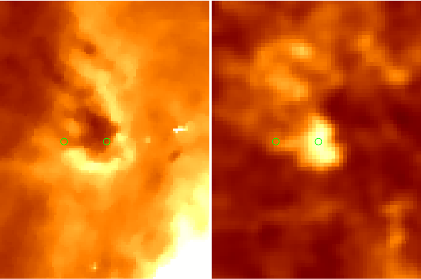
Figure 7: H$\alpha$ map (left) and 100 $\mu$m map (right). Our on and off positions are shown as green circles.

3.2 Polarization Signal

With the GBT at 9 GHz we have determined that $Q=35\pm 30\,{\rm\mu K}$ and $U=26\pm 34\,{\rm\mu K}$. Figure 6 shows the joint two-parameter $68.3\%$, $95.4\%$, and $99.7\%$ confidence regions for fractional $Q$ and $U$. We employ a simple Maximum Likelihood approach to set a limit on the total linear polarization that avoids the Rice bias. The likelihood of a linear polarization $p=\sqrt{Q^{2}+U^{2}}$ and polarization angle $\theta$ given statistically independent data $Q_{obs},U_{obs}$ is

$$L(p,\theta|Q_{obs},U_{obs})\propto Exp\left[-\left(\frac{(Q-Q_{obs})^{2}}{2\sigma_{Q_{obs}}^{2}}+\frac{(U-U_{obs})^{2}}{2\sigma_{U_{obs}}^{2}}\right)\right]$$ (1)

where $Q=p\,cos\,2\theta$ and $U=p\,sin\,2\theta$. Marginalizing over the position angle of polarization we have

$$L(p|Q_{obs},U_{obs})\propto\int\,d\theta\,Exp\left[-\left(\frac{(Q-Q_{obs})^{2}}{2\sigma_{Q}^{2}}+\frac{(U-U_{obs})^{2}}{2\sigma_{U}^{2}}\right)\right]$$ (2)

The PDF is normalized to unity, and confidence intervals are determined by integrating the PDF. We find $95.4\%$ and $99.7\&$ upper limits on the total linear polarization $p$ of $88\,{\rm\mu K}$ and $123\,{\rm\mu K}$, respectively. For a nominal Stokes I dust signal of $3.5\pm 0.5\,{\rm mK}$ (§ 3.1), and assuming that the free-free signal is unpolarized, these limits correspond to fractional linear polarizations of $2.7\%$ and $3.5\%$.

These limits are consistent with the results of Battistelli et al. on Perseus, who find a fractional linear polarization of $3.4^{+1.5}_{-1.9}\%$. If electric dipole emission is primarily responsible for the observed microwave excess, a population of small dust grains is required, with tyipcal radii of a few nm. These grains can be efficiently aligned by paramagnetic resonance relaxation (Lazarian & Draine 2000), which would give rise to up to $\sim 5\%$ fractional linear polarization at 9 GHz. Both our result and that of Battistelli et al. are lower than this, but probably within theoretical uncertainties. In contrast, magnetic dipole fluctuations in larger, single-domain ferrous grains will show a fractional linear polarization $\sim 10\%$ below 10 GHz, flipping orientation and rising to as much as 33% at 100 GHz (Draine & Lazarian 1999). Many of the magnetic dipole models are excluded by our measurements.

4 Conclusions

We have presented a $9.65$ GHz limit on linear polarization towards the dark cloud Lynds 1622, a well-measured locus of anomalous Galactic microwave emission; the total degree of linear polarization is $<88\,{\rm\mu K}$ at $2\sigma$ ($<123\,{\rm\mu K}$ at $3\sigma$). Assuming a $3.5\,{\rm mK}$ stokes I spinning dust signal, consistent with independent measurements of L1622 at 8 through 32 GHz (Finkbeiner et al., 2002; Casassus et al., 2006), and that the free-free signal is unpolarized, we have limits on the degree of linear polarization of $2.7\%$ and $3.5\%$. These limits are consistent with the expected linear polarization of small rotating grains, and with the 3% fractional linear polarization measured by Battistelli et al. towards Perseus, but inconsistent with many models for the anomalous emission based on magnetic dipole fluctuations in ferrous grains. Such low levels of linear polarization would also be unusual for soft, dust-correlated synchrotron, which has been suggested as a possible origin for the generally observed anomalous microwave emission (Bennett et al., 2003). For L1622, however, soft synchrotron was already strongly ruled out by existing total intensity data. In addition we see that the total intensity signal on the line of sight to L1622 is fainter than on the nearby comparison (Off-source) region. The negative signal we observe is consistent with the level of free-free fluctuations in the region: considering the expected $+3.5$ mK signal, the observed -5 mK signal indicates an $8.5$ mK gradient between our ON and OFF positions, consistent with our estimate of $\pm 5\,{\rm mK}$ variations over the region from H$\alpha$ maps. This underscores the need for good frequency coverage in attempts to charactize the spinning dust foreground at low microwave frequencies. The relatively weak polarization signal observed in L1622 and Perseus bodes well for future CMB polarization experiments. It should be appreciated that while these concentrated loci of emission are important first steps on the road to understanding the anomalous microwave emission, the physical conditions are quite different from those in the diffuse ISM, where foreground properties are most important for future CMB expreiments. To study these regions more sensitive observations are necessary.

The National Radio Astronomy Observatory is a facility of the National Science Foundation operated under cooperative agreement by Associated Universities, Inc.

References

- Banday et al. (2003) Banday, A. J., Dickinson, C., Davies, R. D., Davis, R. J., & Górski, K. M. 2003, MNRAS, 345, 897
- Battistelli et al. (2006) Battistelli, E. S., Rebolo, R., Rubiño-Martín, J. A., Hildebrandt, S. R., Watson, R. A., Gutiérrez, C., & Hoyland, R. J. 2006, ApJ, 645, L141
- Bennett et al. (2003) Bennett, C. L., Hill, R. S., Hinshaw, G., Nolta, M. R., Odegard, N., Page, L., Spergel, D. N., Weiland, J. L., Wright, E. L., Halpern, M., Jarosik, N., Kogut, A., Limon, M., Meyer, S. S., Tucker, G. S., & Wollack, E. 2003, ApJS, 148, 97
- Casassus et al. (2006) Casassus, S., Cabrera, G. F., Förster, F., Pearson, T. J., Readhead, A. C. S., & Dickinson, C. 2006, ApJ, 639, 951
- Casassus et al. (2004) Casassus, S., Readhead, A. C. S., Pearson, T. J., Nyman, L.-Å., Shepherd, M. C., & Bronfman, L. 2004, ApJ, 603, 599
- Davies et al. (2006) Davies, R. D., Dickinson, C., Banday, A. J., Jaffe, T. R., Górski, K. M., & Davis, R. J. 2006, MNRAS, 370, 1125
- de Oliveira-Costa et al. (1997) de Oliveira-Costa, A., Kogut, A., Devlin, M. J., Netterfield, C. B., Page, L. A., & Wollack, E. J. 1997, ApJ, 482, L17+
- de Oliveira-Costa et al. (2004) de Oliveira-Costa, A., Tegmark, M., Davies, R. D., Gutiérrez, C. M., Lasenby, A. N., Rebolo, R., & Watson, R. A. 2004, ApJ, 606, L89
- de Oliveira-Costa et al. (2002) de Oliveira-Costa, A., Tegmark, M., Finkbeiner, D. P., Davies, R. D., Gutierrez, C. M., Haffner, L. M., Jones, A. W., Lasenby, A. N., Rebolo, R., Reynolds, R. J., Tufte, S. L., & Watson, R. A. 2002, ApJ, 567, 363
- de Oliveira-Costa et al. (1998) de Oliveira-Costa, A., Tegmark, M., Page, L. A., & Boughn, S. P. 1998, ApJ, 509, L9
- Dickinson et al. (2003) Dickinson, C., Davies, R. D., & Davis, R. J. 2003, MNRAS, 341, 369
- Draine & Lazarian (1998a) Draine, B. T. & Lazarian, A. 1998a, ApJ, 494, L19+
- Draine & Lazarian (1998b) —. 1998b, ApJ, 508, 157
- Draine & Lazarian (1999) —. 1999, ApJ, 512, 740
- Erickson (1957) Erickson, W. C. 1957, ApJ, 126, 480
- Finkbeiner et al. (1999) Finkbeiner, D. P., Davis, M., & Schlegel, D. J. 1999, ApJ, 524, 867
- Finkbeiner et al. (2004) Finkbeiner, D. P., Langston, G. I., & Minter, A. H. 2004, ApJ, 617, 350
- Finkbeiner et al. (2002) Finkbeiner, D. P., Schlegel, D. J., Frank, C., & Heiles, C. 2002, ApJ, 566, 898
- Gaustad et al. (2001) Gaustad, J. E., McCullough, P. R., Rosing, W., & Van Buren, D. 2001, PASP, 113, 1326
- Heiles (2001) Heiles, C. 2001, PASP, 113, 1243
- Heiles et al. (2001a) Heiles, C., Perillat, P., Nolan, M., Lorimer, D., Bhat, R., Ghosh, T., Howell, E., Lewis, M., O’Neil, K., Salter, C., & Stanimirovic, S. 2001a, PASP, 113, 1247
- Heiles et al. (2001b) Heiles, C., Perillat, P., Nolan, M., Lorimer, D., Bhat, R., Ghosh, T., Lewis, M., O’Neil, K., Salter, C., & Stanimirovic, S. 2001b, PASP, 113, 1274
- Kogut et al. (1996) Kogut, A., Banday, A. J., Bennett, C. L., Gorski, K. M., Hinshaw, G., Smoot, G. F., & Wright, E. I. 1996, ApJ, 464, L5+
- Lazarian & Draine (2000) Lazarian, A. & Draine, B. T. 2000, ApJ, 536, L15
- Leitch et al. (1997) Leitch, E. M., Readhead, A. C. S., Pearson, T. J., & Myers, S. T. 1997, ApJ, 486, L23+
- Miville-Deschênes & Lagache (2005) Miville-Deschênes, M.-A. & Lagache, G. 2005, ApJS, 157, 302
- Schlegel et al. (1998) Schlegel, D. J., Finkbeiner, D. P., & Davis, M. 1998, ApJ, 500, 525
- Watson et al. (2005) Watson, R. A., Rebolo, R., Rubiño-Martín, J. A., Hildebrandt, S., Gutiérrez, C. M., Fernández-Cerezo, S., Hoyland, R. J., & Battistelli, E. S. 2005, ApJ, 624, L89