A state-space mixed membership blockmodel for dynamic network tomography

Abstract

In a dynamic social or biological environment, the interactions between the actors can undergo large and systematic changes. In this paper we propose a model-based approach to analyze what we will refer to as the dynamic tomography of such time-evolving networks. Our approach offers an intuitive but powerful tool to infer the semantic underpinnings of each actor, such as its social roles or biological functions, underlying the observed network topologies. Our model builds on earlier work on a mixed membership stochastic blockmodel for static networks, and the state-space model for tracking object trajectory. It overcomes a major limitation of many current network inference techniques, which assume that each actor plays a unique and invariant role that accounts for all its interactions with other actors; instead, our method models the role of each actor as a time-evolving mixed membership vector that allows actors to behave differently over time and carry out different roles/functions when interacting with different peers, which is closer to reality. We present an efficient algorithm for approximate inference and learning using our model; and we applied our model to analyze a social network between monks (i.e., the Sampson’s network), a dynamic email communication network between the Enron employees, and a rewiring gene interaction network of fruit fly collected during its full life cycle. In all cases, our model reveals interesting patterns of the dynamic roles of the actors.

, and tfSupported by Grant ONR N000140910758, NSF DBI-0640543, NSF DBI-0546594, NSF IIS-0713379, DARPA CS Futures II award, and an Alfred P. Sloan Research Fellowship.

1 Introduction

Networks are a fundamental form of representation of complex systems. In many problems arising in biology, social sciences, and various other fields, it is often necessary to analyze populations of entities such as molecules or individuals, also known as “actors” in some network literature, interconnected by a set of relationships such as regulatory interactions, friendships, and communications. Studying networks of these kinds can reveal a wide range of information, such as how molecules/individuals organize themselves into groups, which molecules are the key regulator or which individuals are in positions of power, and how the patterns of biological regulations or social interactions are likely to evolve over time.

In this paper we investigate an intriguing statistical inference problem of interpreting the dynamic behavior of temporally evolving networks based on a concept known as network tomography. Borrowed from the vocabulary of magnetic resonance imaging, the term “network tomography” was first introduced by Vardi (1996) to refer to the study of a network’s internal characteristics using information derived from the observed network. In most real-world complex systems such as a social network or a gene regulation network, the measurable attributes and relationships of vertices (or nodes) in a network are often functions of latent temporal processes of events which can fluctuate, evolve, emerge, and terminate stochastically. Here we define network tomography more specifically as the latent semantic underpinnings of entities in both static and dynamic networks. For example, it can stand for the latent class labels, social roles, or biological functions undertaken by the nodal entities, or the measures on the affinity, compatibility, and cooperativity between nodal states that determine the edge probability. Our goal is to develop a statistical model and algorithms with which such information can be inferred from dynamically evolving networks via posterior inference.

We will concern ourselves with three specific real world time-evolving networks in our empirical analysis: (1) the well-known Sampson’s undirected social networks [Sampson (1969)] of 18 monks over 3 time episodes, which are recorded during an interesting timeframe that preludes a major conflict followed by a mass departure of the monks, and therefore an interesting example case to infer nodal causes behind dramatic social changes; (2) the time series of email-communication networks of ENRON employees before and during the collapse of the company, which may have recorded interesting and perhaps sociologically illuminating behavioral patterns and trends under various business operation conditions; and (3) the sequence of gene interaction networks estimated at 22 time points during the life span of Drosophila melanogaster, a fruit fly commonly used as a lab model to study the mechanisms of animal embryo development, which captures transient regulatory events such as the animal aging.

Inference of network tomography is fundamental for understanding the organization and function of complex relational structures in natural, sociocultural, and technological systems such as the ones mentioned above. In a social system such as a company employee network, network tomography can capture the latent social roles of individuals; inferring such roles based on the social interactions among individuals is fundamental for understanding the importance of members in a network, for interpreting the social structure of various communities in a network, and for modeling the behavioral, sociological, and even epidemiological processes mediated by the vertices in a network. In systems biology, network tomography often translates to latent biochemical or genetic functions of interacting molecules such as proteins, mRNAs, or metabolites in a regulatory circuity; elucidating such functions based on the topology of molecular networks can advance our understanding of the mechanisms of how a complex biological system regulates itself and reacts to stimuli. More broadly, network tomography can lead to important insights to the robustness of network structures and their vulnerabilities, the cause and consequence of information diffusion, and the mechanism of hierarchy and organization formation. By appropriately modeling network tomography, a network analyzer can also simulate and reason about the generative mechanisms of networks, and discover changing roles among actors in networks, which will be relevant for activity and anomaly detection.

There has been a variety of successes in network analysis based on various formalisms. For example, researchers have found trends in a wide variety of large-scale networks, including scale-free and small-world properties [Barabasi and Albert (1999); Kleinberg (2000)]. Other successes include the formal characterization of otherwise intuitive notions, such as “groupness” which can be formally characterized in the networks perspective using measures of structural cohesiveness and embeddedness [Moody and White (2003)], detecting outbreaks [Leskovec et al. (2007)], and characterizing macroscopic properties of various large social and information networks [Leskovec et al. (2008)]. Additionally, there has been progress in statistical modeling of social networks, traditionally focusing on descriptive models such as the exponential random graph models, and more recently moving toward various latent space models that estimate an embedding of the network in a latent semantic space, as we review shortly in Section 2. A major limitation of most current methods for network modeling and inference [Hoff, Raftery and Handcock (2002); Li and McCallum (2006); Handcock, Raftery and Tantrum (2007)] is that they assume each actor, such as a social individual or a biological molecule in a network, undertakes a single and invariant role (or functionality, class label, etc., depending on the domain of interest), when interacting with other actors. In many realistic social and biological scenarios, every actor can play multiple roles (or under multiple influences) and the specific role being played depends on whom the actor is interacting with; and the roles undertaken by an actor can change over time. For example, during a developmental process or an immune response in a biological system, there may exist multiple underlying “themes” that determine the functionalities of each molecule and their relationships to each other, and such themes are dynamical and stochastic. As a result, the molecular networks at each time point are context-dependent and can undergo systematic rewiring, rather than being i.i.d. samples from a single underlying distribution, as assumed in most current biological network studies. We are interested in understanding the mechanisms that drive the temporal rewiring of biological networks during various cellular and physiological processes, and similar phenomena in time-varying social networks.

In this paper we propose a new Bayesian approach for network tomographic inference that will capture the multi-facet, context-specific, and temporal nature of an actor’s role in large, heterogeneous, and evolving dynamic networks. The proposed method will build on a modified version of the mixed membership stochastic blockmodel (MMSB) [Airoldi et al. (2008)], which enables network links to be realized by role-specific local connection mechanisms; each link is underlined by a separately chosen latent functional cause, and each vertex can have fractional involvement in multiple functions or roles which are captured by a mixed membership vector, thereby the proposed model supports analyzing patterns of interactions between actors via statistically inferring an “embedding” of a network in a latent “tomographic-space” via the mixed membership vectors. For example, the characteristics of group profiles of actors revealed by the mixed membership vectors can offer important and intuitive community structures in the networks in question.

Modeling embedding of networks in latent state space offers an intuitive but powerful approach to infer the semantic underpinnings of each actor, such as its biological or social roles or other entity functions, underlying the observed network topologies. Via such a model, one can map every actor in a network to a position in a low-dimensional simplex, where the roles/functions of the actors are reflected in the role- or functional-coordinates of the actors in the latent space and the relationships among actors are reflected in their Euclidian distances. We can naturally capture the dynamics of role evolution of actors in such a tomographic-space, and other latent dynamic processes driving the network evolution by furthermore applying a state-space model (SSM) popular in object tracking over the positions of the tomographic-embeddings of all actors, where a logistic-normal mixed membership stochastic blockmodel is employed as the emission model to define time-specific condition likelihood of the observed networks over time. The resulting model shall be formally known as a state-space mixed membership stochastic blockmodel, but, for simplicity, in this paper we will refer to it as a dynamic MMSB (or, in short, dMMSB); and we will show that this model allows one to infer the trajectory of the roles of each actor based on the posterior distribution of its role-vector.

Given network data, the dMMSB can be learned based on the maximum likelihood principle using a variational EM algorithm [Ghahramani and Beal (2001); Xing, Jordan and Russell (2003); Ahmed and Xing (2007)], the resulting network parameters reveal not only mixed membership information of each actor over time, but also other interesting regularities in the network topology. We will illustrate this model on the well-known Sampson’s monk social network, and then apply it to the time series of email network from Enron and the sequence of time-varying genetic interaction networks estimated from the Drosophila genome-wise microarray time series, and we will present some previously unnoticed dynamic behaviors of network actors in these data.

The remaining part of the paper is organized as follows. In Section 2 we briefly review some related work. In Section 3 we present the dMMSB model in detail. A Laplace variational EM algorithm for approximate inference under dMMSB will be described in Section 4. In Section 5 we present case studies on the monks network, the Enron network, and the Drosophila gene network using dMMSB, along with some simulation based validation of the model. Some discussions will be given in Section 6. Algebraic details of the derivations of the inference algorithm are provided in the Appendix.

2 Related work

There is a vast and growing body of literature on model-based statistical analysis of network data, traditionally focusing on descriptive models such as the exponential random graph models (ERGMs) [Frank and Strauss (1986); Wasserman and Pattison (1996)], and more recently moving toward more generative types of models such as those that model the network structure as being caused by the actors’ positions in a latent “social space” [Hoff, Raftery and Handcock (2002)]. Among these models, some variants of the ERGMs, such as the stochastic block models [Holland, Laskey and Leinhardt (1983); Fienberg, Meyer and Wasserman (1985); Wasserman and Pattison (1996); Snijders (2002)], cluster network vertices based on their structural equivalency [Lorrain and White (1971)]. The latent space models (LSM) instead project nodes onto a latent space, where their similarities can be visualized and explored [Hoff, Raftery and Handcock (2002); Hoff (2003); Handcock, Raftery and Tantrum (2007)]. The mixed membership stochastic blockmodel proposed in Airoldi et al. (2005, 2008) integrates ideas from these models, but went further by allowing each node to belong to multiple blocks (i.e., groups) with fractional membership. Variants of the mixed membership model have appeared in population genetics [Pritchard, Stephens and Donnelly (2000)], text modeling [Blei, Jordan and Ng (2003)], analysis of multiple disability measures [Erosheva and Fienberg (2005)], etc. In most of these cases mixed membership models are used as a latent-space projection method to project high-dimensional attribute data into a lower-dimensional “aspect-space,” as a normalized mixed membership vector, which reflects the weight of each latent aspect (e.g., roles, functions, topics, etc.) associated with an object [Erosheva, Fienberg and Lafferty (2004)]. The mixed membership vectors often serve as a surrogate of the original data for subsequent analysis such as classification [Blei, Ng and Jordan (2003)]. The MMSB model developed earlier has been applied for role identification in Sampson’s 18-monk social network and functional prediction in a protein–protein interaction network (PPI) [Airoldi et al. (2005, 2008)]. It uses the aforementioned mixed membership vector to define an actor-specific multinomial distribution, from which specific actor roles can be sampled when interacting with other actors. For each monk, it yields a multi-class social-identity prediction which captures the fact that his interactions with different other monks may be under different social contexts. For each protein, it yields a multi-class functional prediction which captures the fact that its interactions with different proteins may be under different functional contexts.

We intend to use the state-space model (SSM) popular in object tracking and trajectory modeling for inferring underlying functional changes in network entities, and sensing emergence and termination of “function themes” underlying network sequences. This scheme has been adopted in a number of recent works on extracting evolving topical themes in text documents [Blei and Lafferty (2006b); Wang and McCallum (2006)] or author embeddings [Sarkar and Moore (2005)] based on author, text, and reference networks of archived publications.

3 Modeling dynamic network tomography

Consider a temporal series of networks $\{{G}^{(1)},\ldots,{G}^{(T)}\}$ over a vertex set $V$, where ${G}^{(t)}\equiv\{V,E^{(t)}\}$ represents the network observed at time $t$. In this paper we assume that $N=|V|$ is invariant over time; thus, ${E}^{(t)}\equiv\{e^{(t)}_{i,j}\}_{i,j=1}^{N}$ denote the set of (possibly transient) links at time $t$ between a fixed set of $N$ vertices.

To model both the multi-class nature of every vertex in a network and the latent semantic characteristics of the vertex-classes and their relationships to inter-vertices interactions, we assume that at any time point, every vertex $v_{i}\in V$ in the network, such as a social actor or a biological molecule, can undertake multiple roles or functions realized from a predefined latent tomographic space according to a time-varying distribution $P_{t}(\cdot)$; and the weights (i.e., proportion of “contribution”) of the involved roles/functions can be represented by a normalized vector $\vec{\pi}^{(t)}_{i}$ of fixed dimension $K$. We refer to each role, function, or other domain-specific semantics underlying the vertices as a membership of a latent class. Earlier stochastic blockmodels of networks restricted each vertex to belong to a single and invariant membership. In this paper we assume that each vertex can have mixed memberships, that is, it can undertake multiple roles/functions within a single network when interacting with various network neighbors with different roles/functions, and the vector of proportions of the mixed-memberships, $\vec{\pi}^{(t)}_{i}$, can evolve over time. Furthermore, we assume that the links between vertices are instantiated stochastically according to a compatibility function over the roles undertaken by the vertex-pair in question, and we define the compatibility coefficients between all possible pair of roles using a time-evolving role-compatibility matrix ${B}^{(t)}\equiv\{\beta^{(t)}_{k,l}\}$.

3.1 Static mixed membership stochastic blockmodel

Under a basic MMSB model, as first proposed in Airoldi et al. (2005), network links can be realized by a role-specific local interaction mechanism: the link between each pair of actors, say, $(i,j)$, is instantiated according to the latent role specifically undertaken by actor $i$ when it is to interact with $j$, and also the latent role of $j$ when it is to interact with $i$. More specifically, suppose that each different role-pair, say, roles $k$ and $l$, between actors has a unique probability distribution $P(\cdot|\beta_{k,l})$ of having a link between actor pairs with that role combination, then a basic mixed membership stochastic blockmodel posits the following generative scheme for a static network:

1. For each vertex $i$, draw the mixed-membership vector: $\vec{\pi}_{i}\sim P(\cdot|\theta)$.

2. For each possible interacting vertex $j$ of vertex $i$, draw the link indicator $e_{i,j}\in\{0,1\}$ as follows:

   • draw latent roles $\vec{z}_{i\rightarrow j}\sim\operatorname{Multinomial}(\cdot|\vec{\pi}_{i},1)$, $\vec{z}_{j\leftarrow i}\sim\operatorname{Multinomial}(\cdot|\vec{\pi}_{j},1)$, where $\vec{z}_{i\rightarrow j}$ denotes the role of actor $i$ when it is to interact with $j$, and $\vec{z}_{j\leftarrow i}$ denotes the role of actor $j$ when it is approached by $i$. Here $\vec{z}_{i\rightarrow j}$ and $\vec{z}_{j\leftarrow i}$ are unit indictor vectors in which one element is one and the rest are zero; it represents the $k$th role if and only if the $k$th element of the vector is one, for example, $z_{i\rightarrow j,k}=1$ or $z_{j\leftarrow i,k}=1$

   • and draw $e_{i,j}|(z_{i\rightarrow j,k}=1,z_{j\leftarrow i,l}=1)\sim\operatorname{Bernoulli}(\cdot|{\beta}_{k,l})$.

Specifically, the generative model above defines a conditional probability distribution of the relations $E=\{e_{i,j}\}$ among vertices in a way that reflects naturally interpretable latent semantics (e.g., roles, functions, cluster identities) of the vertices. The link $e_{i,j}$ represents a binary actor-to-actor relationship. For example, the existence of a link could mean that a package has been sent from one person to another, or one has a positive impression on another, or one gene is regulated by another. Each vertex $v_{i}$ is associated with a set of latent membership labels $\{\vec{z}_{i\rightarrow\cdot},\vec{z}_{i\leftarrow\cdot}\}$ (if the links are undirected, as in a PPI, then we can ignore the asymmetry of “$\rightarrow$” and “$\leftarrow$”). Thus, the semantic underpinning of each interaction between vertices is captured by a pair of instantiated memberships unique to this interaction; and the nature and strength of the interaction is controlled by the compatibility function determined by this pair of memberships’ instantiation. For example, if actors A and C are of role $X$ while actors B and D are of role $Y$, we may expect that the relationship from A to B is likely to be the same as relationship from C to D, because both of them are from a role-$X$ actor to a role-$Y$ actor. In this sense, a role is like a class label in a classification task. However, under an MMSB model, an actor can have different role instantiations when interacting with different neighbors in the same network.

The role-compatibility matrix ${B}\equiv\{\beta_{k,l}\}$ decides the affinity between roles. In some cases, the diagonal elements of the matrix may dominate over other elements, which means actors of the same role are more likely to connect to each other. In the case where we need to model differential preference among different roles, richer block patterns can be encoded in the role-compatibility matrix. The flexibility of the choices of the $B$ matrix give rise to strong expressivity of the model to deal with complex relational patterns. If necessary, a prior distribution over elements in $B$ can be introduced, which can offer desirable smoothing or regularization effects.

Crucial to our goal of role-prediction and role-evolution modeling for network data is the so-called mixed membership vector ${\vec{\pi}}_{i}$, also referred to as “role vector,” of the mixed-membership coefficients in the above generative model, which represents the overall role spectrum of each actor and succinctly captures the probabilities of an actor involving in different roles when this actor interacts with another actor. Much of the expressiveness of the mixed-membership models lies in the choice of the prior distribution for the mixed-membership coefficients ${\vec{\pi}}_{i}$, and the prior for the interaction coefficients $\{\beta_{k,l}\}$. For example, in Airoldi et al. (2005, 2008), a simple Dirichlet prior was employed because it is conjugate to the multinomial distribution over every latent membership label $\{\vec{z}_{i\rightarrow\cdot},\vec{z}_{i\leftarrow\cdot}\}$ defined by the relevant $\vec{\pi}_{i}$. In this paper, to capture nontrivial correlations among the weights (i.e., the individual elements within ${\vec{\pi}}_{i}$) of all latent roles of a vertex, and to allow one to introduce dynamics to the roles of each actor when modeling temporal processes such as a cell cycle, we employ a logistic-normal distribution over a simplex [Aitchison and Shen (1980); Aitchison (1986); Ahmed and Xing (2007)]. The resulting model is referred to as a logistic-normal MMSB, or simply LNMMSB.

Under a logistic normal prior, assuming a centered logistic transformation, the first sampling step for $\vec{\pi}_{i}\equiv[\pi_{i,1},\ldots,\pi_{i,K}]$ in the canonical mixed membership generative model above can be broken down into two sub-steps: first draw $\vec{\gamma}_{i}$ according to

$$\vec{\gamma}_{i}\sim\operatorname{Normal}(\vec{\mu},\Sigma);$$ (1)

then map it to the simplex via the following logistic transformation:

$$\pi_{i,k}=\operatorname{exp}\{\gamma_{i,k}-C({\vec{\gamma}}_{i})\}\qquad\forall k=1,\ldots,K,$$ (2)

where

$$C({\vec{\gamma}}_{i})=\log\Biggl{(}\sum_{k=1}^{K}\operatorname{exp}\{\gamma_{i,k}\}\Biggr{)}.$$ (3)

Here $C({\vec{\gamma}}_{i})$ is a normalization constant (i.e., the log partition function). Due to the normalizability constrain of the multinomial parameters, $\vec{\pi}_{i}$ only has $K-1$ degree of freedom. Thus, we only need to draw the first $K-1$ components of $\vec{\gamma}_{i}$ from a $(K-1)$-dimensional multivariate Gaussian, and leave $\gamma_{i,K}=0$. For simplicity, we omit this technicality in the forthcoming general description and operation of our model.

Under a dynamic network tomography model, the prior distributions of role weights of every vertex $P_{t}(\cdot),$ and the role-compatibility matrix $B$, can both evolve over time. Conditioning on the observed network sequence $\{{G}^{(1)},\ldots,{G}^{(T)}\}$, our goal is to infer the trajectories of role vectors $\vec{\pi}^{(t)}_{i}$ in the latent social space or biological function space. In the following, we present a generative model built on elements from the classical state-space model for linear dynamic systems and the static logistic normal MMSB described above for random graphs for this purpose.

3.2 Dynamic logistic-normal mixed membership stochastic blockmodel

We propose to capture the dynamics of network evolution at the level of both the prior distributions of the mixed membership vectors of vertices, and the compatibility functions governing role-to-role relationships. In this way we capture the dynamic behavior of the generative system of both vertices and relations. Our basic model structure is based on the well-known state-space model, which defines a linear dynamic transformation of the mixed membership priors over adjacent time points:

$$\vec{\mu}^{(t)}=\mathbf{A}\vec{\mu}^{(t-1)}+\vec{w}^{(t)}\qquad\mbox{for }t\geq 1,$$ (4)

where $\vec{\mu}^{(t)}$ represents the mean parameter of the prior distribution of the transformed mixed membership vectors of all vertices at time $t$, and $\vec{w}^{(t)}\sim\mathcal{N}(0,\Phi)$ represents normal transition noise for the mixed membership prior, and the transition matrix $\mathbf{A}$ shapes the trajectory of temporal transformation of the prior. The LNMMSB model defined above now functions as an emission model within the SSM that defines the conditional likelihood of the network at each time point. Note that the linear system on $\vec{\mu}^{(t)}$ can lead to a bursty dynamics for latent admixing vector $\pi^{(t)}_{i}$ through the LNMMSB emission model. Starting from this basic structure, we propose to develop a dynamical model for tracking underlying functional changes in network entities and sensing emergence and termination of “function themes.”

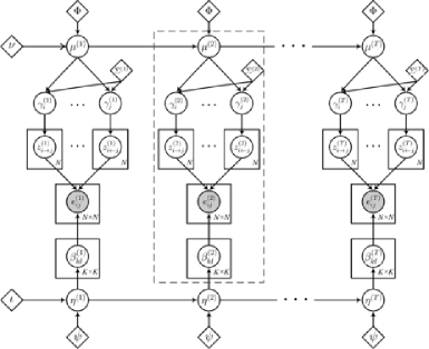
Figure 1: A graphical model representation of the dynamic logistic-normal mixed membership stochastic blockmodel. The part enclosed by the dotted lines is a logistic-normal MMSB.

Given a sequence of network topologies over the same set of nodes, here is an outline of the generative process under such a model (a graphical model representation of this model is illustrated in Figure 1):

• State-space model for mixed membership prior:

  • $\vec{\mu}^{(1)}\sim\operatorname{Normal}(\nu,\Phi)$, sample the mean of the mixed membership prior at time 1.

  For $t=1,\ldots,T$:

  • $\vec{\mu}^{(t)}=\operatorname{Normal}(\mathbf{A}\vec{\mu}^{(t-1)},\Phi)$, sample the means of the mixed membership priors over time.

• State-space model for role-compatibility matrix:

• For $k=1,\ldots,K$ and $k^{\prime}=1,\ldots,K$,

  • ${\eta}_{k,k^{\prime}}^{(1)}\sim\operatorname{Normal}(\iota,\psi)$, sample the compatibility coefficient between role $k$ and $k^{\prime}$ at time 1.

  For $t=1,\ldots,T$:

  • ${\eta}_{k,k^{\prime}}^{(t)}\sim\operatorname{Normal}(b\eta_{k,k^{\prime}}^{(t-1)},\psi)$, sample compatibility coefficients over subsequent time points.

  • $\beta_{k,k^{\prime}}^{(t)}={\exp(\eta_{k,k^{\prime}}^{(t)})}/{(\exp(\eta_{k,k^{\prime}}^{(t)})+1)}$, compute compatibility probabilities via logistic transformation.

• Logistic-normal mixture membership model for networks:

• For each node $n=1,\ldots,N$, at each time point $t=1,\ldots,T$:

  • $\vec{\pi}^{(t)}_{i}\sim\operatorname{LogisticNormal}(\vec{\mu}^{(t)},\Sigma^{(t)})$, sample a $k$ dimensional mixed membership vector.

  For each pair of nodes $(i,j)\in[1,N]\times[1,N]$:

  • ${\vec{z}_{i\rightarrow j}}^{(t)}\sim\operatorname{Multinomial}(\vec{\pi}^{(t)}_{i},1)$, sample membership indicator for the donor,

  • ${\vec{z}_{j\leftarrow i}}^{(t)}\sim\operatorname{Multinomial}(\vec{\pi}^{(t)}_{j},1)$, sample membership indicator for the acceptor,

  • $e^{(t)}_{i,j}\sim\operatorname{Bernoulli}({\vec{z}_{i\rightarrow j}}^{(t)\prime}B^{(t)}{\vec{z}_{j\leftarrow i}}^{(t)})$, sample the links between nodes.

Specifically, we assume that the mixed membership vector $\vec{\pi}$ for each actor follows a time-specific logistic normal prior $\mathcal{LN}({\vec{\mu}}^{(t)},\Sigma^{(t)})$, whose mean ${\vec{\mu}}^{(t)}$ is evolving over time according to a linear Gaussian model. For simplicity, we assume that the $\Sigma^{(t)}$ which captures time-specific topic correlations is independent across time.

It is noteworthy that unlike a standard SSM of which the latent state would emit a single output (i.e., an observation or a measurement) at each time point, the dMMSB model outlined above generates $N$ emissions each time, one corresponding to the (pre-transformed) mixed-membership vector $\vec{\gamma}_{i}^{(t)}$ of each vertex. To directly apply the Kalman filter and Rauch–Tung–Striebel smoother for posterior inference and parameter estimation under dMMSB, we introduce an intermediate random variable $\vec{Y}^{(t)}=\frac{1}{N}\sum_{i}\vec{\gamma}_{i}^{(t)}$; it is easy to see that $\vec{Y}^{(t)}$ follows a standard SSM reparameterized from the original dMMSB:

$$\vec{Y}^{(t)}\sim\operatorname{Normal}\biggl{(}\vec{\mu}^{(t)},\frac{\Sigma^{(t)}}{N}\biggr{)}\qquad t=1,\ldots,T.$$ (5)

In principle, we can use the above membership evolution model to capture not only membership correlation within and between vertices at a specific time [as did in Blei and Lafferty (2006a)], but also dynamic coupling (i.e., co-evolution) of membership proportions via covariance matrix $\Phi$. In the simplest scenario, when $\mathbf{A}=I$ and $\Phi=\sigma I$, this model reduces to a random walk in the membership-mixing space. Since in most realistic temporal series of networks both the role-compatibility functions between vertices and the semantic representations of membership-mixing are unlikely to be invariant over time, we expect that even a random walk mixed-membership evolution model can provide a better fit of the data than a static model that ignores the time stamps of all networks.

4 Variational inference

Due to difficulties in marginalization over the super-exponential state space of latent variables $\vec{\mathbf{z}}$ and $\vec{\pi}$, even the basic MMSB model based on a Dirichlet prior over the role vectors $\vec{\pi}$ is intractable [Airoldi et al. (2005, 2008)]. With the additional difficulty in integration of $\vec{\pi}$ under a logistic normal prior where a closed-form solution is unavailable, exact posterior inference of the latent variables of interest and direct EM estimation of the model parameters is infeasible. In this section we present a Laplace variational approximation scheme based on the generalized means field (GMF) theorem [Xing, Jordan and Russell (2003)] to infer the latent variables and estimate the model parameters. This scheme requires one additional approximating step on top of the variational approximation developed in Airoldi et al. (2008), but we will show empirically in Section 5.1.1 that this step does not introduce much additional error. The GMF approach is modular, that is, we can approximate the joint posterior $p(\{\vec{\mathbf{z}}^{(t)},\vec{\pi}^{(t)},\vec{\mu}^{(t)},B^{(t)}\}_{t=1}^{T}|\Theta,\{G^{(t)}\}_{t=1}^{T})$, where $\Theta$ denotes the model parameters, by a factored approximate distribution:

$$q\bigl{(}\bigl{\{}\vec{\mathbf{z}}^{(t)},\vec{\pi}^{(t)},\vec{\mu}^{(t)},B^{(t)}\bigr{\}}_{t=1}^{T}\bigr{)}$$

(6)

$$\qquad=q_{1}\bigl{(}\bigl{\{}\vec{\mathbf{z}}^{(t)},\vec{\pi}^{(t)}\bigr{\}}_{t=1}^{T}\bigr{)}q_{2}\bigl{(}\bigl{\{}\vec{\mu}^{(t)}\bigr{\}}_{t=1}^{T}\bigr{)}q_{3}\bigl{(}\bigl{\{}B^{(t)}\bigr{\}}_{t=1}^{T}\bigr{)},$$

where $q_{1}(\cdot)$ can be shown to be the marginal distribution of $\{\vec{\mathbf{z}}^{(t)},\vec{\pi}^{(t)}\}_{t=1}^{T}$ under a reparameterized LNMMSB, and $q_{2}(\cdot)$ and $q_{3}(\cdot)$ are SSMs over $\{\vec{\mu}^{(t)}\}_{t=1}^{T}$ and $\{B^{(t)}\}_{t=1}^{T}$, respectively, with emissions related to expectation of $\{\vec{\mathbf{z}}^{(t)},\vec{\pi}^{(t)}\}_{t=1}^{T}$ under $q_{1}(\cdot)$. This can be shown by minimizing the Kulback–Leibler divergence between $q(\cdot)$ and $p(\cdot)$ over arbitrary choices of $q_{1}(\cdot)$, $q_{2}(\cdot)$, and $q_{3}(\cdot)$, as proven in Xing, Jordan and Russell (2003). The computation of the variational parameters of each of these approximate marginals leads to a coupling of all the marginals, as apparent in the descriptions in the subsequent subsections. But once the variational parameters are solved, inference on any latent variable of interest under the joint distribution $p(\cdot)$, which is intractable, can be approximated by a much simpler inference on the same variable in one of the $q_{i}(\cdot)$ marginals that contains the variables of interest. Below we briefly outline solutions to each of these marginals of subset of variables, which exactly correspond to the three building blocks of the dMMSB model outlined in Section 3.2. [Since $\mu^{(t)}$ and $B^{(t)}$ both follow a standard SSM, for simplicity, we only show the solution to $q_{2}(\cdot)$ over $\mu^{(t)}$, and treat $B^{(t)}$ as an unknown invariant constant to be estimated.]

4.1 Variational approximation to logistic-normal MMSB

For a static MMSB, the inference problem is to estimate the role-vectors given model parameters and observations. That is, model parameters $\vec{\mu}$, $\Sigma$, and $B$ are assumed to be known besides the observed variables $E$, and we want to compute estimates of the role vectors $\vec{\gamma}_{\cdot}$ along with role indicators $\vec{z}_{\cdot\rightarrow\cdot}$ and $\vec{z}_{\cdot\leftarrow\cdot}$. (Under dMMSB, $\vec{\mu}$ is in fact unknown, but we will discuss shortly how to estimate it outside of the MMSB inference detailed below.)

Under the LNMMSB, ignoring time and vertex indices, the marginal posterior of latent variables $\vec{\gamma}$ (the pretransformed $\vec{\pi}$) and $\vec{\mathbf{z}}$ is

$$p(\vec{\gamma}_{\cdot},\vec{z}_{\cdot\rightarrow\cdot},\vec{z}_{\cdot\leftarrow\cdot}|\vec{\mu},\Sigma,B,E)$$

$$\qquad\propto\prod_{i}p(\vec{\gamma}_{i}|\vec{\mu},\Sigma)\prod_{i,j}p(\vec{z}_{i\rightarrow j},\vec{z}_{j\leftarrow i}|\vec{\gamma}_{i},\vec{\gamma}_{j})p(e_{ij}|\vec{z}_{i\rightarrow j},\vec{z}_{j\leftarrow i},B).$$

Marginalization over all but one hidden variable to predict, say, $\vec{\gamma}_{i}$, is intractable under the above model. Based on the GMF theory, we approximate $p(\vec{\gamma}_{\cdot},\vec{z}_{\cdot\rightarrow\cdot},\vec{z}_{\cdot\leftarrow\cdot}|\vec{\mu},\Sigma,B,E)$ with a product of simpler marginals $q(\cdot)=q_{\gamma}(\cdot)q_{z}(\cdot)$, each on a cluster of latent variable subsets, that is, $\{\vec{\gamma}_{i}\}$ and $\{\vec{z}_{i\rightarrow j},\break\vec{z}_{j\leftarrow i}\}$. Xing, Jordan and Russell (2003) proved that under GMF approximation, the optimal solution, $q(\cdot)$, of each marginal over the cluster of variables is isomorphic to the true conditional distribution of the cluster given its expected Markov Blanket. That is,

$$q_{\gamma}(\vec{\gamma}_{i}) = p(\vec{\gamma}_{i}|\vec{\mu},\Sigma,\langle{\vec{z}_{i\rightarrow\cdot}}\rangle_{q_{z}},\langle{\vec{z}_{i\leftarrow\cdot}}\rangle_{q_{z}}),$$ (8)

$$q_{z}(\vec{z}_{i\rightarrow j},\vec{z}_{j\leftarrow i}) = p(\vec{z}_{i\rightarrow j},\vec{z}_{j\leftarrow i}|e_{ij},B,\langle{\vec{\gamma}_{i}}\rangle_{q_{\gamma}},\langle{\vec{\gamma}_{j}}\rangle_{q_{\gamma}}).$$ (9)

These equations define a fixed point for $q_{\gamma}$ and $q_{z}$. The optimal marginal distribution of the variables in one cluster is updated when we fix the marginal of all the other variables, in turn. The update continues until the change is neglectable.

The update formula for a cluster marginal of ($\vec{z}_{i\rightarrow j}$, $\vec{z}_{j\leftarrow i}$) is straightforward. It follows a multinomial distribution with $K\times K$ possible outcomes:

$$\hskip 25.0ptq_{z}(\vec{z}_{i\rightarrow j},\vec{z}_{j\leftarrow i}) \propto p(\vec{z}_{i\rightarrow j}|\langle{\vec{\gamma}_{i}}\rangle_{q_{\gamma}})p(\vec{z}_{j\leftarrow i}|\langle{\vec{\gamma}_{j}}\rangle_{q_{\gamma}})p(e_{ij}|\vec{z}_{i\rightarrow j},\vec{z}_{j\leftarrow i},B)$$

$$\sim \operatorname{Multinomial}(\vec{\delta}_{ij}),$$

where $\delta_{ij(u,v)}\equiv\frac{1}{C}\exp(\langle{\gamma_{i,u}}\rangle_{q_{\gamma}}+\langle{\gamma_{j,v}}\rangle_{q_{\gamma}})\beta_{u,v}^{e_{ij}}(1-\beta_{u,v})^{1-e_{ij}}$, and $C$ is the normalization function to keep $\sum_{(u,v)}\delta_{ij(u,v)}=1$. Furthermore, the expectation of $z$’s according to the multinomial distribution are

$${\langle z_{i\rightarrow j,u}\rangle}_{q_{z}} = \frac{\sum_{v}\delta_{ij(u,v)}}{\sum_{u,v}\delta_{ij(u,v)}}=\sum_{v}\delta_{ij(u,v)},$$

$${\langle z_{j\leftarrow i,v}\rangle}_{q_{z}} = \frac{\sum_{u}\delta_{ij(u,v)}}{\sum_{u,v}\delta_{ij(u,v)}}=\sum_{u}\delta_{ij(u,v)}.$$

The update formula for $\vec{\gamma}_{i}$ can be derived similarly, but some further approximation is applied. First,

$$q_{\gamma}(\vec{\gamma}_{i}) \propto p(\vec{\gamma}_{i}|\vec{\mu},\Sigma)p(\langle{\vec{z}_{i\rightarrow\cdot}}\rangle_{q_{z}},\langle{\vec{z}_{i\leftarrow\cdot}}\rangle_{q_{z}}|\vec{\gamma}_{i})$$

$$= \mathcal{N}(\vec{\gamma}_{i};\vec{\mu},\Sigma)\exp\bigl{(}{\langle{\vec{m}_{i}}\rangle_{q_{z}}^{T}}\vec{\gamma_{i}}-(2N-2)C(\vec{\gamma_{i}})\bigr{)},$$

where $m_{ik}=\sum_{j\neq i}(z_{i\rightarrow j,k}+z_{i\leftarrow j,k})$, $\langle{m_{ik}}\rangle_{q_{z}}=\sum_{j\neq i}^{N}(\langle{z_{i\rightarrow j,k}}\rangle_{q_{z}}+\langle{z_{i\leftarrow j,k}}\rangle_{q_{z}})$, and $C(\vec{\gamma_{i}})=\log(\sum_{k=1}^{K}\exp\{\gamma_{i,k}\})$. The presence of the normalization constant $C(\vec{\gamma}_{i})$ makes $q_{\gamma}$ unintegrable in the closed-form. Therefore, we apply a Laplace approximation to $C(\vec{\gamma}_{i})$ based on a second-order Taylor expansion around $\hat{\gamma_{i}}$ [Ahmed and Xing (2007)], such that $q_{\gamma}(\vec{\gamma}_{i})$ becomes a reparameterized multivariate normal distribution $\mathcal{N}(\tilde{\gamma}_{i},\tilde{\Sigma}_{i})$ (see Appendix .1 for details). In order to get a good approximation, the point of expansion, $\hat{\gamma_{i}}$, should be set as close to the query point as possible. Therefore, we set it to be the $\tilde{\gamma}_{i}$ obtained from the previous iteration, that is, $\hat{\gamma}_{i}^{r+1}=\tilde{\gamma}_{i}^{r}$ where $r$ denotes the iteration number.

The inference algorithm iterates between equation (4.1) and equation (4.1) until convergence when the relative change of log-likelihood is less than $10^{-6}$ in absolute value. The procedure is repeated multiple times with random initialization for $\tilde{\gamma}_{i}$. The result having the best likelihood is picked as the solution.

4.2 Parameter estimation for logistic-normal MMSB

The model parameters $\vec{\mu}$, $\Sigma$, and $B$ have to be estimated from data $E\equiv\{e_{ij}\}$. In the simplest case, where time evolution of $\vec{\mu}$ and $B$ is ignored, these can be done via a straightforward EM-style procedure.

In the E-step, we use the inference algorithm from Section 4.1 to compute the posterior distribution and expectation of the latent variables by fixing the current parameters. In the M-step, we re-estimate the parameters by maximizing the log-likelihood of the data using the posteriors obtained from the E-step. Under a LNMMSB, exact computation of the log-likelihood is intractable, hence, we use an approximation method known as variational EM. We obtain the following update formulas for variational EM [Ghahramani and Beal (2001)] (see Appendix .2 for an illustration of the derivation of the update for $B$):

$$\hat{\beta}_{k,l} = \frac{\sum_{i,j}e_{ij}\delta_{ij(k,l)}}{\sum_{i,j}\delta_{ij(k,l)}},\qquad\hat{\mu}=\frac{1}{N}\sum_{i}\tilde{\gamma}_{i},$$

$$\hat{\Sigma} = \frac{1}{N}\sum_{i}\tilde{\Sigma}_{i}+\operatorname{Cov}(\tilde{\gamma}_{1:N}).$$

The procedure for the learning can be summarized below.

Learning for logistic-normal MMSB:

1. initialize $B\sim\mathcal{U}[0,1]$, $\vec{\mu}~{}\sim\mathcal{N}(0,I)$, $\Sigma=10I$

2. while not converged (Outer Loop)

   1. [2.1.]

   2. Initialize $q(\vec{\gamma}_{i})$

   3. while not converged and #iteration $\leq$ threshold (Inner Loop)

      1. [2.2.1.]

      2. update $q(\vec{z}_{i\rightarrow j},\vec{z}_{j\leftarrow i})\sim\operatorname{Multinomial}(\vec{\delta}_{ij})$

      3. update $q(\vec{\gamma}_{i})\sim\mathcal{N}(\tilde{\gamma}_{i},\tilde{\Sigma}_{i})$

      4. update $B$

   4. update $\vec{\mu},\Sigma$

The convergence criterion is the same as in inference. It is worth noting that the update of role-compatibility matrix $B$ is in the inner loop, which means that it is updated as frequently as mixed membership vectors $\vec{\gamma}_{i}$. This makes sense because the role-compatibility matrix and mixed membership vectors are closely coupled.

4.3 Variational approximation to dMMSB

When $\vec{\mu}$ is time-evolving as in dMMSB, two aspects in the algorithms described in Sections 4.1 and 4.2 need to be treated differently. First, unlike in equation (4.2), estimation of $\vec{\mu}^{(t)}$ now must be done under an SSM, with $\{\tilde{\gamma}^{(t)}_{i}\}$ as the emissions at every time point. Second, according to the GMF theorem, the $\mu$ that appeared in all equations in Section 4.1 must now be replaced by the posterior mean of $\vec{\mu}^{(t)}$ under this SSM. Below we first summarize the algorithm for dMMSB, followed by details of the update steps based on the Kalman Filter (KF) and the Rauch–Tung–Striebel (RTS) smoother algorithms.

Inference for dMMSB:

1. initialize all $\vec{\mu}^{(t)}$

2. while not converged

   1. [2.1.]

   2. for each $t$

      1. [2.1.1.]

      2. call the inference algorithm for MMSB on network ${E}^{(t)}$ in Section 4.1 (by passing to it all current estimate of $\vec{\mu}^{(t)}$), and return the GMF approximation $\tilde{\gamma}_{i}^{(t)},\tilde{\Sigma}_{i}^{(t)}$

      3. update the observations, $\vec{Y}^{(t)}=\sum_{i}\tilde{\gamma}_{i}^{(t)}/N$

   3. RTS smoother update $\vec{\mu}^{(t)}=\hat{\mu}_{t|T}$ based on $\{\vec{Y}^{(t)}\}_{t=1}^{T}$

Given all model parameters and all the emissions (the current estimate of the mixed membership vectors $\{\tilde{\gamma}^{(t)}_{i}\}$ of all vertices returned by the logistic-normal MMSB at each time point), posterior inference of the hidden states $\vec{\mu}^{(t)}$ can be solved according to the following KF and RTS procedure. The major update steps in the Kalman Filter are as follows:

$$\hat{\mu}_{t+1|t} = A\hat{\mu}_{t|t}=\hat{\mu}_{t|t},$$

$$P_{t+1|t} = AP_{t|t}A^{T}+\Phi=P_{t|t}+\Phi,$$

$$K_{t+1} = P_{t+1|t}(P_{t+1|t}+\Sigma_{t+1}/N)^{-1},$$

$$\hat{\mu}_{t+1|t+1} = \hat{\mu}_{t+1|t}+K_{t+1}(\vec{Y}_{t+1}-\hat{\mu}_{t+1|t}),$$ (14)

$$P_{t+1|t+1} = P_{t+1|t}-K_{t+1}P_{t+1|t},$$ (15)

where $\hat{\mu}_{t|s}\equiv\mathbb{E}(\vec{\mu}^{(t)}|\vec{Y}_{1},\ldots,\vec{Y}_{s})$ and $P_{t|s}\equiv\operatorname{Var}(\vec{\mu}^{(t)}|\vec{Y}_{1},\ldots,\vec{Y}_{s})$. And the major update steps in the Rauch–Tung–Striebel smoother are as follows:

$$L_{t} = P_{t|t}A^{T}P_{t+1|t}^{-1}=P_{t|t}P_{t+1|t}^{-1},$$

$$\hat{\mu}_{t|T} = \hat{\mu}_{t|t}+L_{t}(\hat{\mu}_{t+1|T}-\hat{\mu}_{t+1|t}),$$ (16)

$$P_{t|T} = P_{t|t}+L_{t}(P_{t+1|T}-P_{t+1|t})L_{t}^{T}.$$ (17)

4.4 Parameter estimation for dMMSB

We again use the variational EM algorithm. The E-step uses the dMMSB inference algorithm in Section 4.3 for computing sufficient statistics $\hat{\mu}_{t|T},\forall t$, and the logistic normal MMSB inference algorithm in Section 4.2 for computing all sufficient statistics $\delta_{ij(k,l)}^{(t)}$. In the M-step, model parameters are updated by maximizing the log-likelihood obtained from the E-step. From this on, we simplify the linear transition model posed on matrix $B$ and assume that it is constant. We derive the following updates for the model parameters $B,\nu,\Phi,\Sigma^{(t)}$ (see Appendix .3 for some details):

$$\hskip 30.0pt\hat{\beta}_{k,l} = \frac{\sum_{t}\sum_{i,j}e_{ij}^{(t)}\delta_{ij(k,l)}^{(t)}}{\sum_{t}\sum_{i,j}\delta_{ij,(k,l)}^{(t)}},$$ (18)

$$\hat{\Phi} = \frac{1}{T-1}\Biggl{(}\sum_{t=1}^{T-1}(\hat{\mu}_{t+1|T}-\hat{\mu}_{t|T})(\hat{\mu}_{t+1|T}-\hat{\mu}_{t|T})^{\tt T}+\sum_{t=1}^{T-1}L_{t}P_{t+1|T}L_{t}^{T}\Biggr{)},$$ (19)

$$\hat{\Sigma}^{(t)} = \frac{1}{N}\biggl{(}\sum_{i}\bigl{(}\hat{\mu}_{t|T}-\tilde{\gamma}_{i}^{(t)}\bigr{)}\bigl{(}\hat{\mu}_{t|T}-\tilde{\gamma}_{i}^{(t)}\bigr{)}^{\tt T}+\sum_{i}\tilde{\Sigma}_{i}^{(t)}\biggr{)},$$ (20)

$$\hat{\nu} = \hat{\mu}_{1|T}.$$ (21)

The algorithm can be summarized below.

Learning for dMMSB:

1. initialize $B\sim\mathcal{U}[0,1]$, $\nu\sim\mathcal{N}(0,I)$, $\vec{\mu}^{(t)}=\nu$, $\Phi=10I$, $\Sigma^{(t)}=10I$

2. while not converged

   1. [2.1.]

   2. initialize all $q(\vec{\gamma}_{i}^{(t)})$

   3. while not converged

      1. [2.2.1.]

      2. for each $t$

         1. [2.2.1.2.]

         2. update $q(\vec{z}_{i\rightarrow j},\vec{z}_{j\leftarrow i})\sim\operatorname{Multinomial}(\vec{\delta}_{ij})$

         3. update $q(\vec{\gamma}_{i})\sim\mathcal{N}(\tilde{\gamma}_{i},\tilde{\Sigma}_{i})$

      3. update $B$

   4. RTS smoother update, $\vec{\mu}^{(t)}=\hat{\mu}_{t|T}$ based on $\{\vec{Y}^{(t)}\}_{t=1}^{T}$

   5. update $\nu,\Phi,\Sigma^{(t)}$

Notice that in the above algorithm, the variational cluster marginals $q(\vec{z}_{i\rightarrow j},\vec{z}_{j\leftarrow i})$, $q(\vec{\gamma}_{i})$, and $q(\vec{\mu}^{(1)},\ldots,\vec{\mu}^{(T)})$ each depend on variational parameters defined by other cluster marginals. Thus, overall the algorithm is essentially a fixed-point iteration that will converge to a local optimum. We use multiple random restarts to obtain a near global optimum.

5 Experiments

In this section we validate the inference algorithms presented in Section 4 on synthetic networks and demonstrate the advantages of the dMMSB model on the well-known Sampson’s monk network. Then we apply dMMSB to two large-scale real world data sets.

5.1 Synthetic networks

We first evaluate the logistic normal MMSB described in Section 3.1 in comparison with the earlier Dirichlet MMSB proposed by Airoldi et al. (2008), and then with the dMMSB model described in Section 3.2. We investigate their differences in three major aspects: (i) Is the Laplace variational inference algorithm adequate for accurately estimating the mixed membership vectors? (ii) For a static network, does LNMMSB provide a better fit to the data when different roles are correlated? And (iii) for dynamic networks, does dMMSB provide a better fit to the data?

5.1.1 Inference accuracy

We generated three sets of synthetic networks, each of which has 100 individuals and 3 roles, using 3 different sets of role-vector priors and role-compatibility matrices, to mimic different real-life situations. Figure 2 shows the estimation errors with LNMMSB under the three scenarios. The results from the Dirichlet MMSB are very close to that of LNMMSB and therefore are not shown here.

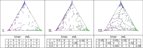
Figure 2: Results of inference and learning with LNMMSB on representative synthetic networks from scenario I to III. In the top row, the figure in each cell displays the estimated role-vectors. They are projected onto a simplex along with the ground truth: a circle represents the position of a ground truth; a cross represents an estimated position; and, each truth-estimation pair is linked by a grey line. Note that we used different colors to denote actors from different groups. In the bottom row, we display the the true and estimated role-compatibility matrices. For all three cases, the estimated role-compatibility matrices are close to the true matrices we used to generate the synthetic networks.

For synthetic network I, most actors have a single role and the role-compatibility matrix is diagonal, which means that actors connect mostly with other actors of the same role. It can be seen that the mixed membership vectors are well recovered. Most of the actors in the simplex are close to a corner, which indicates that they have a dominating role. Some actors are not close to a corner but close to an edge, which means that they have strong memberships for two roles. The remaining actors lying near the center of the simplex have mixed memberships for all three roles. In general, the difficulty of recovering the mixed membership vector increases as an actor possesses more roles.

In synthetic network II, the true mixed membership vector is qualitatively similar to synthetic network I, but the role-compatibility matrix contains off-diagonal entries. As a result, an actor in network II is more likely to connect with actors of a different role than network I. In this more difficult case, our model still accurately estimates the role-compatibility matrix and the mixed membership vectors.

In synthetic network III, we present a very difficult case where many actors undertake noticeable mixed roles, and the within-role affinity is very weak. Though a few actors near the center of the simplex endure obvious discrepancy between the truth and the estimation, less than 10 percent of actors have more than 20 percent errors in their role vectors. Furthermore, we can see the group structure is still clearly retained.

Note that LNMMSB and Dirichlet MMSB employ different variational schemes to approximate the posterior of the mixed membership vectors, and the two models possess different modeling power to accommodate correlations between different memberships. The combined effect could lead to a difference in their accuracy of estimating the mixed membership vectors of every vertex, although in practice we found such difference hardly noticeable in the simplexial display given in Figure 2. To provide a quantitative comparison between the LNMMSB and the Dirichlet MMSB, we compute the average distance between the ground truth and the estimated mixed membership vectors in the aforementioned three settings. We used both the $\ell_{1}$ and the $\ell_{2}$ distance as the metrics in our comparison, and the results are shown in Figure 3, where each type of network is instantiated ten times to produce the error bar. We can see that the LNMMSB performs slightly better for networks I and II (though no significant difference is observed).

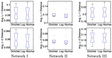
Figure 3: The average distance in (top) L-1 and (bottom) L-2 between the ground truth and the estimation of the mixed membership vectors in networks that share parameter settings as simulation networks I, II and III (from left to right).

5.1.2 Goodness of fit of LNMMSB

To evaluate the fitness of the model to the data, we compute the log-likelihood of fitting a type-II synthetic network generated in the previous experiment, achieved by the model in question at convergence of parameter estimation via the variational EM. Since no simple form of the log-likelihood can be derived for both methods, the log-likelihoods were obtained via importance sampling. The results for LNMMSB and Dirichlet MMSB are listed in Table 1, showing that the goodness of fit of the two models are comparable, with LNMMSB slightly dominating over Dirichlet MMSB. As parallel evidence, the $\ell_{2}$ norm distances between the inferred mixed membership vectors and the ground truth are also shown.

=7.2cm Prior Avg. $\bolds{\ell_{2}}$ distance Log-likelihood Dirichlet 0.091 $-$5755.8 Logistic normal 0.092 $-$5691.7

Table 1: Dirichlet vs. logistic normal prior for MMSB

5.1.3 Goodness of fit of dMMSB

To assess the fitness of the dMMSB, we generate dynamic networks consisting of 10 time points. The number of actors remains 100 and the number of roles remains 3. Furthermore, we generate the networks in such a way that networks between adjacent time points show certain degrees of similarity. As an illustration, the true role compatibility matrix and the mixed membership vectors at time point 6 are displayed in Figure 4.

In Figure 4 (right), we compare dMMSB to an LNMMSB learning a static network for each time point separately. We measure the performance in terms of the average $\ell_{2}$ distance between the estimates of the mixed membership vectors and their true values. It can be seen that the error of dMMSB is lower than the error of MMSB in most cases and about 10 percent lower on average. This suggests that dMMSB can indeed integrate information across temporal domain and better models the networks. More settings of model parameters have been tested on both LNMMSB and dMMSB; they confirm that dMMSB is more effective in modeling dynamic networks.

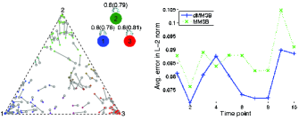
Figure 4: Left: The true mixed membership vectors (circle) and the estimates by dMMSB (cross) at time point 6 visualized in a 2-simplex; each truth-estimate pair is linked by a grey line. Middle: The learned role compatibility matrix, whose nonzero entries are shown by arcs with values; values outside the brackets are the truths and the values inside the brackets are estimates. Right: Average $\ell_{2}$ errors of mixed membership vectors for MMSB and dMMSB.

5.2 Sampson’s monk network: Emerging crisis in a cloister

Now we illustrate the dMMSB model on a small-scale pedagogical example, the Sampson network. Sampson (1969) recorded the social interactions among a group of monks while being a resident in a monastery. He collected a lot of sociometric rankings on relations such as liking, esteem, praise, etc. Toward the end of his study, a major conflict broke out and was followed up by a mass departure of the members. The unique timing of the study makes the data more interesting in the attempt to look for omens of the separation.

We analyze the networks of liking relationship at three time points. They contain 18 members (only junior monks). The networks are directed rather than undirected, because one can like another while not vice versa.

We start with a static analysis on the network of time point 3, which is the latest record before the crisis. Several researchers have also studied the static network, including Breiger, Boorman and Arabie (1975), White, Boorman and Breiger (1976), and Airoldi et al. (2008).

The network is fitted by our model with 1 to 5 roles. The proper number of roles is selected by Bayesian Information Criterion (BIC).

Figure 5 shows the posterior estimation of mixed membership vectors of the monks in the monk liking networks by LNMMSB with three roles. It clearly suggests three groups, each of which is close to one vertex of the triangle. Using Sampson’s labels, the three groups correspond to the Young Turks (monks numbered 1, 2, 7, 12, 14, 15, 16), the Loyal Opposition (4, 5, 6, 9, 11) $+$ Waverers (8, 10), and the Outcasts (3, 17, 18) $+$ Waverer (13). The result is consistent with all previous works except for a controversial person, Mark (13). He is known as an interstitial member of the monastery. Breiger, Boorman and Arabie (1975) placed him with the Loyal Opposition, whereas White, Boorman and Breiger (1976) and Airoldi et al. (2008) placed him among the Outcasts.

Figure 6(a) demonstrates the estimated role-compatibility matrix. It appears that the inter-group relation of liking is strong, while the intra-group relation is absent. Together with the fact that most of the individuals have an almost pure role, it suggests that an explicit boundary exists between the groups, leaving the later separation as no surprise. Figure 6(b) gives the BIC scores. It suggests that the model with 3 roles is the best.

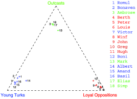
Figure 5: Posterior mixed membership vectors of the monks projected in a 2-simplex by Log-Normal MMSB with 3 roles. Numbered points can be mapped to monks’ names using the legend on the right. Colors identify the composition of mixed membership role-vectors.

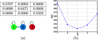
Figure 6: (a) The estimated role-compatibility matrix of the monk liking networks by Log-Normal MMSB with 3 roles. (b) The Bayesian Information Criterion scores of the learning result of the monk liking network with 1 to 5 roles. The lower the better.

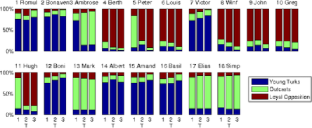
Figure 7: The role-vectors learned in the dynamic network of liking relationship between members in the Sampson Monastery. Each color represents a role.

The trajectories of the varying role-vectors over time inferred by dMMSB with three roles are illustrated in Figure 7. Several big changes in mixed membership vectors happened from time 1 to time 2, and some minor fluctuation occurred between time 2 and time 3. Overall, most persons were stable in the dominant role. If we only look at time 3, which is the one we studied earlier in the static network analysis, the results of mixed membership and grouping of the two models are mostly consistent. Therefore, according to the discussion in the static network analysis, the three roles in the dynamic model can be roughly interpreted as Young Turks, Loyal Opposition, and Outcasts.

One of the persons whose dominant role changed is Ambrose (3). He later became an Outcast. However, at time 1, he was connected with both Romul (1) and Bonaven (2) in the Young Turks besides his connection with Elias (17), an Outcast. It supports our result viewing him mainly as a Young Turk at the time. The other two persons are Peter (5) and Hugh (11). They were close to some Outcasts at time 1 but flipped to Loyal Opposition at time 2, where they finally belonged to. It suggests that the Outcast group whose member finally got expelled had not been noticeably formed until after these big changes happened between time 1 and time 2.

From time 2 to time 3, it can be observed that the mixed membership vectors were purifying, for instances, in monks numbered 1, 3–10, 12, and 15–17. Bonaven (2) and Albert (14) were the exceptions, but they did not change the general trend. The purifying process indicated that the members of different groups were more and more isolated, which finally led to the outbreak of a major conflict.

5.3 Analysis of Enron email networks

Now we study the Enron email communication networks. The email data was processed by Shetty and Adibi (2004). We further extract email senders and recipients in order to build email networks. We have processed the data such that numerous email aliases are properly corresponded to actual persons.

There are 151 persons in the data set. We used emails from 2001, and built an email network for each month, so the dynamic network has 12 time points. We learn a dMMSB of 5 latent roles. The composition and trajectory of roles of each recorded company employee and the role compatibility matrix are depicted in Figure 8.

It is observed that the first role (blue) stands for inactivity, that is, the condition that a vertex is not interacting with any peers; this is a necessary role to account for the intrinsic sparsity of the network. The other roles are active. Actors with Role 2 (cyan), likely representing lower-level employees, only send email to persons of the same role, therefore, they form a clique. So is Role 4 (orange), which leads to another clique. Persons #6, 9, 48, 67, etc. mainly assume this role, and they communicate with many others in the same role. They appear to be normal employees according to available information and the underlying meaning of the clique is yet to be discovered.

Role 5 (red) is within the functional composition of many people. Persons in Role 5 send emails to persons with either Role 5 or Role 3 (green). They form a large clique, where Role 3 corresponds to receivers and Role 5 to both senders and receivers. Role 3 might reflect a certain aspect of senior management role that routinely receives reports/instructions, while Role 5 might correspond to an executive role that likes to issue orders to the managers and communicate among themselves, or other level of positions that behave somewhat similarly but possibly with opposite purpose, for example, reporting to managers rather than dominating over them.

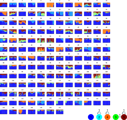
Figure 8: Temporal changes of the mixed membership vectors for each actor, and the visualization for role compatibility matrix.

Of special interest are individuals that are frequently dominated by multiple active roles (especially those falling into separate cliques), because they have strong connection with different groups and may serve important positions in the company. By scanning Figure 8, actor #65 and #107 fit best to this category. According to external sources, Mark Haedicke (#65) was the Managing Director of the Legal Department and Louise Kitchen (#107) was the President of Enron Online, which supports the finding by our method.

We also zoom into Kenneth Lay (#127), the Chairman and CEO of Enron at the time. His role vector in August is abnormally dominated by Role 3, which stands for a receiver. It is exactly the time when Enron’s financial flaws were first publicly disclosed by an analyst, which might lead to a massive increase in enquiry emails from the internal employees.

With respect to systematic changes in temporal space, the role vectors of most actors are smooth over time. However, a few people experience a large increase in the weight of the inactivity role in December (i.e., persons #6, 13, 36, 67, 76). This is the time when Enron filed for bankruptcy.

We can also visualize the mixed membership vectors of the network entities and track the trajectory of the mixed membership vector for an individual as shown in Figure 9. They can help us understand the network as a whole and how each individual evolves in his or her role. Based on these examples, we believe dMMSB can provide a useful visual portal for exploring the stories behind Enron.

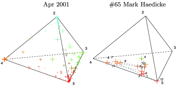
Figure 9: Left: Visualization of mixed membership vectors of network actors in 3-simplex at one time point. Each vertex of the tetrahedron corresponds to a role marked by its ID. A mixed membership vector is represented by a cross whose location and color are the weighted average of its active roles and whose size is proportional to the sum of the weights from the active roles. Right: We track the trajectory of the mixed membership vector for an actor across time. Numbers in italics show time stamps.

5.4 Analysis of evolving gene network as fruit fly aging

In this section we study a sequence of gene correlation networks of the fruit fly Drosophila melanogaster estimated at various point of its life cycle. It is known that over the developmental course of any complex organism, there exist multiple underlying “themes” that determine the functionalities of each gene and their relationships to each other, and such themes are dynamical and stochastic. As a result, the gene regulatory networks at each time point are context-dependent and can undergo systematic rewiring, rather than being invariant over time. We expect the dMMSB model can capture such properties in the time-evolving gene networks of Drosophila melanogaster.

However, experimentally uncovering the topology of the gene network at multiple time points as the animal aging is beyond current technology. Here we used the time-evolving networks of Drosophila melanogaster reverse-engineered by Kolar et al. (2010) from a genome-wide microarray time series of gene expressions using a novel computational algorithm based on $\ell_{1}$ regularized kernel reweighting regression, which is detailed in a companion paper that also appears in this issue. Altogether, 22 networks at different time points across various developmental stages, namely, embryonic stage (1–10 time point), larval stage (11–13 time point), pupal stage (14–19 time points), and adult stages (20–22 time points), are analyzed. We focused on 588 genes that are known to be related to the developmental process based on their gene ontologies.

We plotted the mixed membership vector over 4 roles for each gene as it varies across the developmental cycle (Figure 10). From the time courses of these mixed membership vectors, we can see that many genes assume very different roles during different stages of the development. In particular, we see that many genes exhibit sharp transition in terms of their roles near the end of the embryonic stage. This is consistent with the underlying developmental requirement of Drosophila that the gene interaction networks need to undergo a drastic reconfiguration to accommodate the new stage of larval development. Somewhat surprisingly, we found when the number of roles is set to four, the probability of interacting between different roles is very small, as revealed by the visualization of the role compatibility matrix (Figure 10, lower right). More experiments are needed to examine whether this pattern is a true property of the Drosophila gene interactions or an experimental artifact (e.g., from accuracy of network reverse engineering, or from the smallish number of roles we have chosen to fit the model, which might be overly coarse, or from the quality of approximate inference in a high-dimensional model).

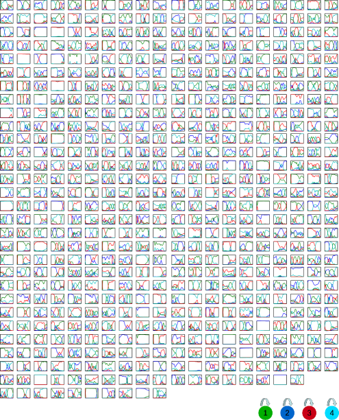
Figure 10: Changes in mixed membership vectors of all genes, and the visualization for role compatibility matrix. The $x$-axes of each subplot is time, and the $y$-axes is the weight of role-component. Each color stands for a role.

We selected four genes for further analysis, namely, Optix, dorsal (dl), lethal (2) essential for life [l(2)efl], and tolkin (tok). These four genes are among the highest degree nodes in the network produced by averaging the dynamic networks over time. We want to see how their roles evolve over time and, therefore, we plotted the trajectory of their mixed membership vector in a 4-d simplex (Figure 11). We can see from the trajectory some of these genes cover a wide area of the 4-d simplex. This is consistent with the roles of gene Optix and dl as transcriptional factors that participate in many different functions and regulate the expression of a wide range of other genes. For instance, dl participates in a diverse range of functions such as anterior/posterior pattern formation, dorsal/ventral axis specification, immune response, gastrulation, heart development; Optix participates in nervous system and compound eye development. In contrast, gene tok and l(2)efl are not transcriptional factors and they are currently only known for very limited functions: tok is related to axon guidance and wing vein morphogenesis; l(2)efl is related to embryonic and heart development. In our results, we found that, indeed, the role-coordinates of tok are almost invariant, but the trajectory of l(2)efl suggests that it may play more diverse roles than what is currently known and deserves further experimental studies.

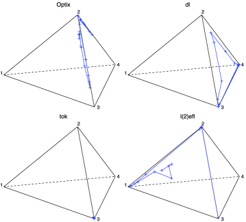
Figure 11: The trajectories of mixed membership vectors of 4 genes [Optix, dl, tok, l(2)efl].

We further used the mixture membership vectors as features to cluster genes at each time point into 4 clusters (each cluster corresponding to a particular role-combination pattern), and studied the gene functions in each role-combination across time. In other words, we try to provide a functional decomposition for each role obtained from the dMMSB model and investigate how these roles evolve over time. In particular, we examined 45 ontological groups and computed the score enrichment of these biological functions over random distribution in each role cluster. Figures 12 and 13 demonstrate the results in cluster (i.e., role) 1. The overall pattern that emerges from our results is that each role consists of genes with a variety of functions, and the functional composition of each role varies across time. However, the distributions over these function groups are very different for different roles: the most common functional groups for genes in role 1 are related to multicellular organismal development, cuticle development, and pigmentation during development; for the second role, the most common functional groups are gland morphogenisis, heart development, gut development, and ommatidial rotation; for the third role, they are stem cell maintenance, sensory organ development, central nervous system development, lymphoid organ development, and gland development; for the fourth role, gastrulation, multicellular organismal development, gut development, stem cell maintenance, and regionalization.

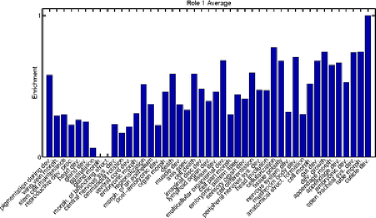
Figure 12: Average gene ontology (GO) enrichment score for role 1. The enrichment score for a given function is the number of genes labeled as this function. Note that in the plot we have normalized the score to a range between $[0,1]$, since we are mainly interested in the relative count for each GO group. Abbreviations appearing in the figure are as follows: dev. for development, proc. for process, morph. for morphogenesis, and sys. for system.

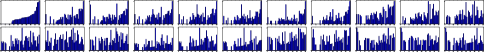
Figure 13: Temporal evolution of gene ontology enrichment score for role 1. The time points are ordered from left to right, and from top to bottom. The order of the gene ontology groups are the same as in Figure 12.

6 Discussion

Unlike traditional descriptive methods for studying networks, which focus on high-level ensemble properties such as degree distribution, motif profile, path length, and node clustering, the dynamic mixed membership stochastic blockmodel proposed in this paper offers an effective way for unveiling detailed tomographical information of every actor and relation in a dynamic social or biological network. This methodology has several distinctive features in its structure and implementation. First, the social or biological roles in the dMMSB model are not independent of each other and they can have their own internal dependency structures; second, an actor in the network can be fractionally assigned to multiple roles; and third, the mixed membership of roles of each actor is allowed to vary temporally. These features provide us extra expressive power to better model networks with rich temporal phenomena.

In practice, this increased modeling power also provides better fit to networks in reality. For instance, the interactions between genes underlying the developmental course of an organism are centered around multiple themes, such as wing development and muscle development, and these themes are tightly related to each other: without the proper development of muscle structures, the development and functionality of wings can not be fulfilled. As an organism moves along its developmental cycle, the underlying themes can evolve and change drastically. For instance, during the embryonic stage of the Drosophila, wing development is simply not present and other processes such as the specification of anterior/posterior axis may be more dominant. Many genes are very versatile in terms of their roles and they differentially interact with different genes depending on the underlying developmental themes. Our model is able to capture these various aspects of the dynamic gene interaction networks, and hence leads us a step further in understanding the biological processes.

In terms of the algorithm, a key ingredient to glue the three features together is the logistic normal prior for the mixed membership vector. This prior is superior to a Dirichlet prior in our context since the off-diagonal entries of the covariance matrix allow us to code the dependency structure between roles, as clearly demonstrated in an earlier work [Ahmed and Xing (2007)]. Another advantage of the logistic normal prior is that it can be readily coupled with a state-space model for tracking the evolution of the roles. However, the drawback of the logistic normal prior is that it is not a conjugate prior to the multinomial distribution and, therefore, additional approximation is needed during learning and inference. For this purpose, we developed an efficient Laplace variational inference algorithm.

Our algorithm scales quadratically with the number of nodes in the network, due to the necessity to infer the context-dependent role indicator $Z$. It scales quadratically with the number of possible roles, and linearly with the number of time steps, which are small compared to the network size. The constant factor typically depends on the stringency of the convergence test in the variational EM and the number of random restarts to alleviate local optimum. In our current implementation, we can handle a network with nodes $\sim$10³ within a day. We have been focusing on developing efficient algorithms that enable dynamic tomographic analysis of “meso-level” networks, that is, a network with thousands of nodes, rather than a “mega” network with millions of nodes. We feel that this objective is appropriate because for mega-networks, such as the blogsphere and the world wide web, it is the ensemble behavior mentioned above that offers more important information to an investigator who wants to do something with the network, rather than individual nodal states. This change of focus with the size of the system can also be seen in economics and game theory.

There are many dimensions where we can extend our current work. For instance, the current model does not explicitly take hubs and cliques of the networks into account, and the state-space model does not enforce temporal smoothness directly over the mixed membership vector but only on its prior. Incorporating these elements will be interesting future research.

Appendix: Derivations

.1 Taylor approximation

We want to approximate $C(\gamma_{i})$ by a second-order Taylor expansion. For simplicity, we temporarily drop the subscript $i$ in this subsection. The Taylor expansion of $C(\vec{\gamma})$ w.r.t. any point $\hat{\gamma}$ is

$$C(\vec{\gamma})\approx C(\hat{\gamma})+{\vec{g}}^{T}(\vec{\gamma}-\hat{\gamma})+\tfrac{1}{2}(\vec{\gamma}-\hat{\gamma})^{T}H(\vec{\gamma}-\hat{\gamma}),$$ (22)

where $\vec{g}$ is the first derivative (a $K\times 1$ vector), and $H$ is the second derivative (a $K\times K$ matrix). Only linear and quadratic terms are left. Therefore, equation (4.1) becomes

$$q_{\gamma}(\vec{\gamma}) \propto \mathcal{N}(\vec{\gamma};\vec{\mu},\Sigma)\exp\bigl{(}{\langle{\vec{m}}\rangle_{q_{z}}^{T}}\vec{\gamma}-(2N-2)C(\vec{\gamma})\bigr{)}$$

$$\approx \exp\bigl{\{}-\tfrac{1}{2}(\vec{\gamma}-\vec{\mu})^{T}\Sigma^{-1}(\vec{\gamma}-\vec{\mu})+{\vec{r}}^{T}\vec{\gamma}+\vec{\gamma}^{T}S\gamma\bigr{\}},$$

where ${\vec{r}}^{T}=\langle{m}\rangle_{q_{z}}^{T}-(2N-2){\vec{g}}^{T}+(2N-2)\hat{\gamma}^{T}H$ is a 1$\times K$ row vector and $S=-(N-1)H$ is a $K\times K$ symmetric matrix.

Letting $x=\vec{\gamma}-\vec{\mu}$, the exponent becomes

$$-\tfrac{1}{2}(\vec{\gamma}-\vec{\mu})^{T}\Sigma^{-1}(\vec{\gamma}-\vec{\mu})+{\vec{r}}^{T}\vec{\gamma}+\vec{\gamma}^{T}S\gamma$$

$$\qquad=-\tfrac{1}{2}x^{T}\Sigma^{-1}x+{\vec{r}}^{T}(x+\vec{\mu})+(x+\vec{\mu})^{T}S(x+\vec{\mu})$$

$$\qquad=-\tfrac{1}{2}x^{T}(\Sigma^{-1}-2S)x+({\vec{r}}^{T}+2{\vec{\mu}}^{T}S)x+C_{1}$$

$$\qquad\phantom{={}}(\mbox{and letting }\tilde{\Sigma}^{-1}=\Sigma^{-1}-2S,D={\vec{r}}^{T}+2{\vec{\mu}}^{T}S)$$

$$\qquad=-\tfrac{1}{2}x^{T}\tilde{\Sigma}^{-1}x+Dx+C_{1}$$

$$\qquad=-\tfrac{1}{2}(x-\tilde{\Sigma}D^{T})^{T}\tilde{\Sigma}^{-1}(x-\tilde{\Sigma}D^{T})+C_{2}$$

$$\qquad=-\tfrac{1}{2}(\vec{\gamma}-\vec{\mu}-\tilde{\Sigma}D^{T})^{T}\tilde{\Sigma}^{-1}(\vec{\gamma}-\vec{\mu}-\tilde{\Sigma}D^{T})+C_{2}.$$

Therefore, $\tilde{\Sigma}=(\Sigma^{-1}-2S)^{-1}=(\Sigma^{-1}+(2N-2)H)^{-1}$

$$\tilde{\gamma} = \vec{\mu}+\tilde{\Sigma}D^{T}=\vec{\mu}+\tilde{\Sigma}(A^{T}+2S\vec{\mu})$$

$$= \vec{\mu}+\tilde{\Sigma}\bigl{(}{\langle\vec{m}_{i}\rangle}_{q_{z}}-(2N-2)\vec{g}+(2N-2)H\hat{\gamma}_{i}-(2N-2)H\vec{\mu}\bigr{)},$$

where the first and the second derivatives are

$$g(\hat{\gamma})_{k} = \frac{\exp\hat{\gamma}_{k}}{\sum_{k}\exp\hat{\gamma}_{k}},$$

$$H(\hat{\gamma})_{kl} = \frac{\mathbb{I}(k=l)}{\sum_{k}\exp\hat{\gamma}_{k}}-\frac{\exp\hat{\gamma}_{k}\exp\hat{\gamma}_{l}}{(\sum_{k}\exp\hat{\gamma}_{k})^{2}}$$

or, in short,

$$H=\operatorname{diag}(\vec{g})-\vec{g}\vec{g}^{T}.$$

.2 Learning on logistic-normal MMSB

The log-likelihood as a function of $B$ can be written as

$$l(B) = \sum_{i,j}\log\sum_{k,l}\bigl{(}\delta_{ij,(k,l)}\beta_{k,l}^{e_{ij}}(1-\beta_{k,l})^{(1-e_{ij})}\bigr{)}+C_{0}$$

$$\geq \sum_{i,j}\sum_{k,l}\delta_{ij,(k,l)}\log\bigl{(}\beta_{k,l}^{e_{ij}}(1-\beta_{k,l})^{(1-e_{ij})}\bigr{)}+C_{0}$$

$$= \sum_{i,j}\sum_{k,l}\delta_{ij,(k,l)}\bigl{(}e_{ij}\log\beta_{k,l}+(1-e_{ij})\log(1-\beta_{k,l})\bigr{)}+C_{0}$$

$$\equiv l^{*}(B),$$

$$\frac{\partial l^{*}(B)}{\partial\beta_{k,l}} = \sum_{i,j}\sum_{k,l}\delta_{ij,(k,l)}\biggl{(}\frac{e_{ij}}{\beta_{k,l}}-\frac{1-e_{ij}}{1-\beta_{k,l}}\biggr{)},$$

$$\hat{\beta}_{k,l} = \frac{\sum_{i,j}e_{ij}\delta_{ij,(k,l)}}{\sum_{i,j}\delta_{ij,(k,l)}}.$$ (24)

Jensen’s Inequality is applied in the derivation to get an approximation (more specifically, a lower bound) to the log-likelihood which has an analytical solution in finding the maximum point. Setting the derivative to zero gives us an MLE estimator of $B$ based on approximation.

.3 Learning on dMMSB

Again, we take an approximation of the log-likelihood, which is more tractable:

$$l(B) = \sum_{t}\sum_{i,j}\log\sum_{k,l}\bigl{(}\delta_{ij,(k,l)}^{(t)}\beta_{k,l}^{e_{ij}^{(t)}}(1-\beta_{k,l})^{(1-e_{ij}^{(t)})}\bigr{)}+C_{0}$$

$$\geq \sum_{t}\sum_{i,j}\sum_{k,l}\delta_{ij,(k,l)}^{(t)}\log\bigl{(}\beta_{k,l}^{e_{ij}^{(t)}}(1-\beta_{k,l})^{(1-e_{ij}^{(t)})}\bigr{)}+C_{0}$$

$$= \sum_{t}\sum_{i,j}\sum_{k,l}\delta_{ij,(k,l)}^{(t)}\bigl{(}e_{ij}^{(t)}\log\beta_{k,l}+\bigl{(}1-e_{ij}^{(t)}\bigr{)}\log(1-\beta_{k,l})\bigr{)}+C_{0}$$

$$\equiv l^{*}(B).$$

The update equation for $B$ is from maximizing the upper bound of the log-likelihood:

$$\frac{\partial l^{*}(B)}{\partial\beta_{k,l}} = \sum_{t}\sum_{i,j}\sum_{k,l}\delta_{ij,(k,l)}^{(t)}\biggl{(}\frac{e_{ij}^{(t)}}{\beta_{k,l}}-\frac{1-e_{ij}^{(t)}}{1-\beta_{k,l}}\biggr{)},$$

$$\hat{\beta}_{k,l} = \frac{\sum_{t}\sum_{i,j}e_{ij}^{(t)}\delta_{ij,(k,l)}^{(t)}}{\sum_{t}\sum_{i,j}\delta_{ij,(k,l)}^{(t)}}.$$ (26)

References

- Ahmed and Xing (2007) Ahmed, A. and Xing, E. P. (2007). On tight approximate inference of logistic-normal admixture model. In Proceedings of the Eleventh International Conference on Artifical Intelligence and Statistics. Omnipress, Madison, WI.
- Airoldi et al. (2005) Airoldi, E., Blei, D., Xing, E. P. and Fienberg, S. (2005). A latent mixed membership model for relational data. In Proceedings of Workshop on Link Discovery: Issues, Approaches and Applications (LinkKDD-2005), The Eleventh ACM SIGKDD International Conference on Knowledge Discovery and Data Mining. Chicago, IL.
- Airoldi et al. (2008) Airoldi, E. M., Blei, D. M., Fienberg, S. E. and Xing, E. P. (2008). Mixed membership stochastic blockmodel. J. Mach. Learn. Res. 9 1981–2014.
- Aitchison (1986) Aitchison, J. (1986). The Statistical Analysis of Compositional Data. Chapman & Hall, New York. \MR0865647
- Aitchison and Shen (1980) Aitchison, J. and Shen, S. M. (1980). Logistic-normal distributions: Some properties and uses. Biometrika 67 261–272. \MR0581723
- Barabasi and Albert (1999) Barabasi, A. L. and Albert, R. (1999). Emergence of scaling in random networks. Science 286 509–512. \MR2091634
- Blei and Lafferty (2006a) Blei, D. and Lafferty, J. (2006a). Correlated topic models. In Advances in Neural Information Processing Systems 18. MIT Press, Boston, MA.
- Blei and Lafferty (2006b) Blei, D. M. and Lafferty, J. D. (2006b). Dynamic topic models. In ICML’06: Proceedings of the 23rd International Conference on Machine Learning 113–120. ACM Press, New York.
- Blei, Jordan and Ng (2003) Blei, D. M., Jordan, M. I. and Ng, A. Y. (2003). Hierarchical Bayesian models for applications in information retrieval. In Bayesian Statistics 7 (J. M. Bernardo, M. J. Bayarri, J. O. Berger, A. P. Dawid, D. Heckerman, A. F. M. Smith and M. West, eds.) 25–44. Oxford Univ. Press. \MR2003181
- Blei, Ng and Jordan (2003) Blei, D. M., Ng, A. and Jordan, M. I. (2003). Latent Dirichlet allocation. J. Mach. Learn. Res. 3 993–1022.
- Breiger, Boorman and Arabie (1975) Breiger, R., Boorman, S. and Arabie, P. (1975). An algorithm for clustering relational data with applications to social network analysis and comparison with multidimensional scaling. J. Math. Psych. 12 328–383.
- Erosheva and Fienberg (2005) Erosheva, E. and Fienberg, S. E. (2005). Bayesian mixed membership models for soft clustering and classification. In Classification—The Ubiquitous Challenge (C. Weihs and W. Gaul, eds.) 11–26. Springer, New York.
- Erosheva, Fienberg and Lafferty (2004) Erosheva, E. A., Fienberg, S. E. and Lafferty, J. (2004). Mixed-membership models of scientific publications. Proc. Natl. Acad. Sci. 97 11885–11892.
- Fienberg, Meyer and Wasserman (1985) Fienberg, S. E., Meyer, M. M. and Wasserman, S. (1985). Statistical analysis of multiple sociometric relations. J. Amer. Statist. Assoc. 80 51–67.
- Frank and Strauss (1986) Frank, O. and Strauss, D. (1986). Markov graphs. J. Amer. Statist. Assoc. 81 832–842. \MR0860518
- Ghahramani and Beal (2001) Ghahramani, Z. and Beal, M. J. (2001). Propagation algorithms for variational Bayesian learning. In Advances in Neural Information Processing Systems 13. MIT Press, Boston, MA.
- Handcock, Raftery and Tantrum (2007) Handcock, M. S., Raftery, A. E. and Tantrum, J. M. (2007). Model-based clustering for social networks. J. Roy. Statist. Soc. Ser. A 170 1–22. \MR2364300
- Hoff (2003) Hoff, P. D. (2003). Bilinear mixed effects models for dyadic data. Technical Report 32, Univ. Washington, Seattle.
- Hoff, Raftery and Handcock (2002) Hoff, P. D., Raftery, A. E. and Handcock, M. S. (2002). Latent space approaches to social network analysis. J. Amer. Statist. Assoc. 97 1090–1098. \MR1951262
- Holland, Laskey and Leinhardt (1983) Holland, P., Laskey, K. B. and Leinhardt, S. (1983). Stochastic blockmodels: Some first steps. Social Networks 5 109–137. \MR0718088
- Kleinberg (2000) Kleinberg, J. (2000). Navigation in a small world. Nature 406 845.
- Kolar et al. (2010) Kolar, M., Song, L., Ahmed, A. and Xing, E. P. (2010). Estimating time-varying networks. Ann. Appl. Statist. 4 94–123.
- Leskovec et al. (2007) Leskovec, J., Krause, A., Guestrin, C., Faloutsos, C., VanBriesen, J. and Glance, N. (2007). Cost-effective outbreak detection in networks. In ACM SIGKDD International Conference on Knowledge Discovery and Data Mining. ACM Press, New York.
- Leskovec et al. (2008) Leskovec, J., Lang, K., Dasgupta, A. and Mahoney, M. (2008). Statistical properties of community structure in large social and information networks. In Proc. 17th International Conference on World Wide Web. ACM Press, New York.
- Li and McCallum (2006) Li, W. and McCallum, A. (2006). Pachinko allocation: Dag-structured mixture models of topic correlations. In ICML’06: Proceedings of the 23rd International Conference on Machine Learning 577–584. ACM Press, New York.
- Lorrain and White (1971) Lorrain, F. and White, H. C. (1971). Structural equivalence of individuals in social networks. J. Math. Soc. 1 49–80.
- Moody and White (2003) Moody, J. and White, D. R. (2003). Structural cohesion and embeddedness: A hierarchical concept of social groups. Amer. Soc. Rev. 68 103–127.
- Pritchard, Stephens and Donnelly (2000) Pritchard, J., Stephens, M. and Donnelly, P. (2000). Inference of population structure using multilocus genotype data. Genetics 155 945–959.
- Sampson (1969) Sampson, S. (1969). Crisis in a cloister. Unpublished doctoral dissertation, Cornell Univ.
- Sarkar and Moore (2005) Sarkar, P. and Moore, A. W. (2005). Dynamic social network analysis using latent space models. SIGKDD Explor. Newsl. 7 31–40.
- Shetty and Adibi (2004) Shetty, J. and Adibi, J. (2004). The Enron email dataset database schema and brief statistical report. Technical report, Information Sciences Institute, Univ. Southern California.
- Snijders (2002) Snijders, T. A. B. (2002). Markov chain Monte Carlo estimation of exponential random graph models. Journal of Social Structure 3.
- Vardi (1996) Vardi, Y. (1996). Network tomography: Estimating source-destination traffic intensities from link data. J. Amer. Statist. Assoc. 91 365–377. \MR1394093
- Wang and McCallum (2006) Wang, X. and McCallum, A. (2006). Topics over time: A non-Markov continuous-time model of topical trends. In KDD’06: Proceedings of the 12th ACM SIGKDD International Conference on Knowledge Discovery and Data Mining 424–433. ACM Press, New York.
- Wasserman and Pattison (1996) Wasserman, S. and Pattison, P. (1996). Logit models and logistic regression for social networks: I. An introduction to Markov graphs and . Psychometrika 61 401–425. \MR1424909
- White, Boorman and Breiger (1976) White, H. C., Boorman, S. A. and Breiger, R. L. (1976). Social structure from multiple networks. I. Blockmodels of roles and positions. Amer. J. Soc. 81 730.
- Xing, Jordan and Russell (2003) Xing, E. P., Jordan, M. I. and Russell, S. (2003). A generalized mean field algorithm for variational inference in exponential families. In Proceedings of the 19th Annual Conference on Uncertainty in AI. Morgan Kaufmann, San Francisco, CA.