Spatial entanglement using a quantum walk on a many-body system

Abstract

The evolution of a many-particle system on a one-dimensional lattice, subjected to a quantum walk can cause spatial entanglement in the lattice position, which can be exploited for quantum information/communication purposes. We demonstrate the evolution of spatial entanglement and its dependence on the quantum coin operation parameters, the number of particles present in the lattice and the number of steps of the quantum walk on the system. Thus, spatial entanglement can be controlled and optimized using a many-particle discrete-time quantum walk.

I Introduction

Entanglement in a quantum state has been the fundamental resource in many quantum information and computation protocols, such as cryptography, communication, teleportation and algorithms NC00 ; HHH09 . To implement these protocols, generating an entangled state is very important. Similarly, studies on the interface between condensed matter systems and quantum information have shown entanglement as a signature of quantum phase transition ON02 ; OAF02 ; OROM06 . To understand the phases and dynamics in many-body systems an analysis of entanglement in many-body systems is very important. Hence, various schemes have been proposed for entanglement generation in quantum systems BH02 ; LHL03 ; RER07 ; WS09 and for understanding entanglement in many-body systems AFOV08 . Quantum walk (QW) is one such process in which an uncorrelated state can evolve to an entangled state and be used to analyze the evolution of entanglement Kem03 ; CLX05 .

The QW, which was developed as a quantum analog of the classical random walk (CRW), evolves a particle into an entanglement between its internal and position degrees of freedom. It has played a significant role in the development of quantum algorithms Amb03 . Furthermore, the QW has been used to demonstrate coherent quantum control over atoms, quantum phase transition CL08 , to explain the phenomena such as breakdown of an electric field-driven system OKA05 and direct experimental evidence for wavelike energy transfer within photosynthetic systems ECR07 ; MRL08 . Experimental implementation of the QW has also been reported DLX03 ; RLB05 ; PLP08 ; KFC09 , and various other schemes have been proposed for its physical realization TM02 ; RKB02 ; EMB05 ; Cha06 ; MBD06 . Therefore, studying entanglement during the QW process will be useful from a quantum information theory perspective and also contribute to further investigation of the practical applications of the QW. In this direction, evolution of entanglement between single particle and position with time (number of steps of the discrete-time QW) has been reported CLX05 .

In this paper, we consider a multipartite quantum walk on a one-dimensional lattice and study the evolution of spatial entanglement, entanglement between different lattice points. All the particles considered in the system are identical and indistinguishable with two internal states (sides of the quantum coin). Spatial entanglement generated using a QW can be controlled by tuning different parameters, such as parameters in the quantum coin operation, number of particles in the system and evolution time (number of steps). To quantify entanglement in the system we are using Meyer-Wallach multipartite entanglement measure.

In Sec. II, we describe single-particle and many-particle discrete-time QWs. In Sec. III, entanglement between a particle and position space and spatial entanglement using single- and many-particle QWs are discussed. In Sec. IV, we present the measure for spatial entanglement of the system using the Meyer-Wallach global entanglement measure scheme for particles in a one-dimensional lattice and in a closed chain ($n-$cycle). We also demonstrate control over spatial entanglement by exploiting the dynamical properties of the QW. We conclude with the summary in Sec. V.

II Quantum Walk

Classical random walk (CRW) describes the dynamics of a particle in position space with a certain probability. The QW is the quantum analog of CRW-developed exploiting features of quantum mechanics such as superposition and interference of quantum amplitudes GVR58 ; FH65 ; ADZ93 . The QW, which involves superposition of states, moves simultaneously exploring multiple possible paths with the amplitudes corresponding to the different paths interfering. This makes the variance of the QW on a line to grow quadratically with the number of steps which is in sharp contrast to the linear growth for the CRW.

The study of QWs has been largely divided into two standard variants: discrete-time QW (DTQW) ADZ93 ; DM96 ; ABN01 and a continuous-time QW (CTQW) FG98 . In the CTQW, the walk is defined directly on the position Hilbert space $\mathcal{H}_{p}$, whereas for the DTQW it is necessary to introduce an additional coin Hilbert space $\mathcal{H}_{c}$, a quantum coin operation to define the direction in which the particle amplitude has to evolve. The connection between these two variants and the generic version of the QW has been studied FS06 ; C08 . However, the coin degree of freedom in the DTQW is an advantage over the CTQW as it allows control of dynamics of the QW AKR05 ; CSL08 . Therefore, we take full advantage of the coin degree of freedom in this work and study the DTQW on a many-particle system.

II.1 Single-particle quantum walk

The DTQW is defined on the Hilbert space $\mathcal{H}=\mathcal{H}_{c}\otimes\mathcal{H}_{p}$. In one dimension, the coin Hilbert space $\mathcal{H}_{c}$, spanned by the basis state $|0\rangle$ and $|1\rangle$, represents two sides of the quantum coin, and the position Hilbert space $\mathcal{H}_{p}$, spanned by the basis states $|\psi_{j}\rangle$, $j\in\mathbb{Z}$, represent the positions in the lattice. To implement the DTQW, we will consider a three-parameter U(2) operator $C_{\xi,\theta,\zeta}$ of the form

$$C_{\xi,\theta,\zeta}\equiv\left(\begin{array}[]{clcr}e^{i\xi}\cos(\theta)&&e^{i\zeta}\sin(\theta)\\ e^{-i\zeta}\sin(\theta)&&-e^{-i\xi}\cos(\theta)\end{array}\right)$$ (1)

as the quantum coin operation CSL08 . The quantum coin operation is applied on the particle state ($C_{\xi,\theta,\zeta}\otimes{\mathbbm{1}}$) when the initial state of the complete system is

$$|\Psi_{in}\rangle=\left[\cos(\delta)|0\rangle+e^{i\eta}\sin(\delta)|1\rangle\right]\otimes|\psi_{0}\rangle.$$ (2)

The state $\cos(\delta)|0\rangle+e^{i\eta}\sin(\delta)|1\rangle$ is the state of the particle and $|\psi_{0}\rangle$ is the state of the position at the lattice position $j=0$.

The quantum coin operation on the particle is followed by the conditional unitary shift operation $S$ which acts on the complete Hilbert space of the system:

$$S=\exp(-i\sigma_{z}\otimes Pl),$$ (3)

where $P$ is the momentum operator, $\sigma_{z}$ is the Pauli spin operator in the $z$ direction and $l$ is the length of each step. The eigenstates of $\sigma_{z}$ are denoted by $|0\rangle$ and $|1\rangle$. Therefore, $S$, which delocalizes the wave packet over the positions $(j-1)$ and $(j+1)$, can also be written as

$$S=|0\rangle\langle 0|\otimes\sum_{j\in\mathbb{Z}}|\psi_{j-1}\rangle\langle\psi_{j}|+|1\rangle\langle 1|\otimes\sum_{j\in\mathbb{Z}}|\psi_{j+1}\rangle\langle\psi_{j}|.$$ (4)

The process of

$$W_{\xi,\theta,\zeta}=S(C_{\xi,\theta,\zeta}\otimes{\mathbbm{1}})$$ (5)

is iterated without resorting to intermediate measurement to help realize a large number of steps of the QW. The parameters $\delta$ and $\eta$ in Eq. (2) can be varied to obtain different initial states of the particle. The three parameters $\xi$, $\theta$ and $\zeta$ of $C_{\xi,\theta,\zeta}$ can be varied to choose the quantum coin operation. By varying parameter $\theta$ the variance can be increased or decreased according to the functional form, $\sigma^{2}\approx(1-\sin(\theta))t^{2}$, where $t$ is the number of steps of the QW, as shown in Fig. 1.

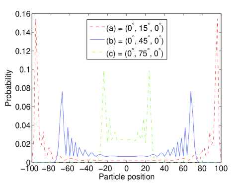
Figure 1: (color online) Spread of the probability distribution for different values of $\theta$ using the quantum coin operator $C_{0,\theta,0}$. The distribution is wider for (a) $(0,\theta,0)=(0,\frac{\pi}{12},0)$ than for (b) $(0,\theta,0)=(0,\frac{\pi}{4},0)$ and (c) $(0,\theta,0)=(0,\frac{5\pi}{12},0)$, showing the decrease in spread with increase in $\theta$. The initial state of the particle is $|\Psi_{ins}\rangle=\frac{1}{\sqrt{2}}\left(|0\rangle+i|1\rangle\right)\otimes|\psi_{0}\rangle$ and the distribution is for 100 steps.

Biased coin operation and biased QW: The most widely studied form of the DTQW is the walk using the Hadamard operation

$$H=\frac{1}{\sqrt{2}}\begin{pmatrix}1&\mbox{~{}}1\\ 1&-1\end{pmatrix},$$ (6)

corresponding to the quantum coin operation with $\xi=\zeta=0$ and $\theta=\pi/4$ in Eq. (1). The Hadamard operation is an unbiased coin operation, and the resulting walk is known as the Hadamard walk. This walk implemented on a particle initially in a symmetric superposition state,

$$|\Psi_{ins}\rangle=\frac{1}{\sqrt{2}}\left[|0\rangle+i|1\rangle\right]\otimes|\psi_{0}\rangle,$$ (7)

obtained by choosing $\delta=\pi/4$ and $\eta=\pi/2$ in Eq. (2), returns a symmetric, unbiased probability distribution of the particle in position space. However, the Hadamard walk on any asymmetric initial state of the particle results in an asymmetric, biased probability distribution of the particle in position space ABN01 . We should note that the role of the initial state on the symmetry of the probability distribution is not vital for a QW using the three-parameter operator given by Eq. (1) as a quantum coin operation.

To elaborate this further, we will consider the first-step evolution of the DTQW using a three-parameter quantum coin operation given by Eq. (1) on a particle initially in the symmetric superposition state. After the first step of the DTQW the state can be written as

$$W_{\xi,\theta,\zeta}|\Psi_{ins}\rangle=\frac{1}{\sqrt{2}}\left[\left(e^{i\xi}\cos(\theta)+ie^{i\zeta}\sin(\theta)\right)|0\rangle|\psi_{-1}\rangle+\left(e^{-i\zeta}\sin(\theta)-ie^{-i\xi}\cos(\theta)\right)|1\rangle|\psi_{+1}\rangle\right].$$ (8)

If $\xi=\zeta$, Eq. (8) has left-right symmetry in the position probability distribution, but not otherwise. That is, the parameters $\xi$ and $\zeta$ introduce asymmetry in the position space probability distribution. Therefore, a coin operation with $\xi\neq\zeta$ in Eq. (1) can be called as a biased quantum coin operation which will bias the QW probability distribution of the particle initially in a symmetric superposition state (Fig. 2) CSL08 . However, we should note that irrespective of the quantum coin operation used, QW can also be biased by choosing an asymmetric initial state of the particle (for example, the Hadamard walk of a particle initially in the state $|0\rangle$ or the state $|1\rangle$).

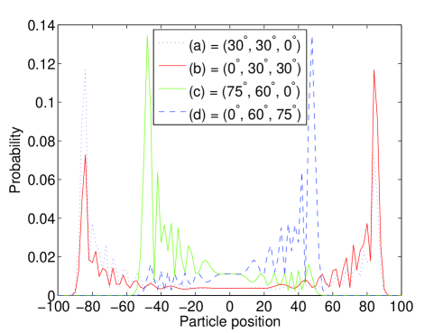
Figure 2: Spread of probability distribution for different values of $\xi$, $\theta$, $\zeta$ using the quantum coin operator $C_{\xi,\theta,\zeta}$. The parameter $\xi$ shifts the distribution to the left: (a)$(\xi,\theta,\zeta)=(\frac{\pi}{6},\frac{\pi}{6},0)$ and (c) $(\xi,\theta,\zeta)=(\frac{5\pi}{12},\frac{\pi}{3},0)$. The parameter $\zeta$ shifts it to the right: (b) $(\xi,\theta,\zeta)=(0,\frac{\pi}{6},\frac{\pi}{6})$ and (d) $(\xi,\theta,\zeta)=(0,\frac{\pi}{3},\frac{5\pi}{12})$. The initial state of the particle $|\Psi_{ins}\rangle=\frac{1}{\sqrt{2}}(|0\rangle+i|1\rangle)\otimes|\psi_{0}\rangle$ and the distribution is for 100 steps.

II.2 Many-particle quantum walk

To define a many-particle QW in one dimension, we will consider an $M$-particle system with one non-interacting particle at each position (Fig. 3). The $M$ identical particles in $M$ lattice points with each particle having its own coin and position Hilbert space will have a total Hilbert space $\mathcal{H}=\left(\mathcal{H}_{c}\otimes\mathcal{H}_{p}\right)^{M}$. We assume the particles to be distinguishable.

The evolution of each step of the QW on the $M$-particle system is given by the application of the operator $W_{0,\theta,0}^{\otimes M}$. The initial state that we will consider for the many-particle system in one dimension will be

$$|\Psi_{ins}^{M}\rangle=\bigotimes_{j=-\frac{M-1}{2}}^{j=\frac{M-1}{2}}\left(\frac{|0\rangle+i|1\rangle}{\sqrt{2}}\right)\otimes|\psi_{j}\rangle.$$ (9)

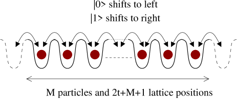
Figure 3: Many-particle state with one non-interacting particle at each position space.

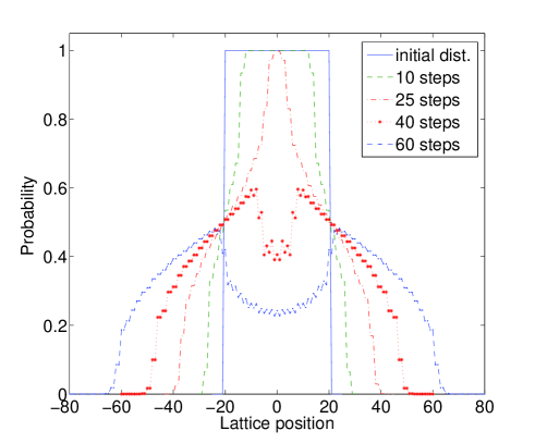
Figure 4: (color online) Probability distribution of 40 particles initially with one particle in each position space when subjected to the QW of different number of steps. The initial state of all the particles is $\frac{1}{\sqrt{2}}(|0\rangle+i|1\rangle)$ and is evolved in position space using the Hadamard operator, $C_{0,\pi/4,0}$ as the quantum coin. The distribution spreads in the position space with an increase in number of steps.

For an $M$-particle system after $t$ steps of the QW, the Hilbert space consists of the tensor product of single lattice position Hilbert space which is $(2t+M+1)$ in number. That is, after $t$ steps of the QW, the $M$ particles are spread between $(j-t)$ to $(j+t)$. In principle, each lattice point is associated with a Hilbert space spanned by two subspaces, a zero-particle subspace and one-particle subspace spanned by two possible states of the coin, $|0\rangle$ and $|1\rangle$. Therefore, the dimension of each lattice point will be $3^{M}$ and the dimension of total Hilbert space is $(3^{M})^{\otimes M}$. Fig. (4) shows the probability distribution of the many-particle system with an increase in number of steps of the QW.

III Entanglement

To efficiently make use of entanglement as a physical resource, the amount of entanglement in a given system has to be quantified. Therefore, entanglement in a pure bipartite system or a system with two Hilbert spaces is quantified using standard measures known as entropy of entanglement or Schmidt number NC00 . The entropy of entanglement corresponds to the von Neumann entropy, a functional of the eigenvalues of the reduced density matrix, and a Schmidt number is the number of non-zero Schmidt coefficients in its Schmidt decomposition. For a multipartite state, there are quite a few good entanglement measures that have been proposed CKW00 ; BL01 ; EB01 ; MW02 ; VDM03 ; Miy08 ; HJ08 . However, as the number of particles in the system increases, the complexity of finding an appropriate entanglement measure also increases, making scalability impractical. Among the proposed measures, to address this scalability problem, Mayer and Wallach proposed a scalable global entanglement measure (polynomial measure) to quantify entanglement in many-particle systems MW02 .

In this section, we will first discuss the entanglement of a particle with position space quantified using entropy of entanglement. Later we will discuss spatial entanglement quantified using the Mayer-Wallach (M-W) measure. Spatial entanglement has been explored earlier using different methods. For example, in an ideal bosonic gas it has been studied using off-diagonal long-range order HAKV07 . For our investigations, we consider a distinguishable many-particle system, implement QW and use the M-W measure to quantify spatial entanglement. In this system the dynamics of particles can be controlled by varying the quantum coin parameters, the initial state of the particles, the number of particles in the system and the number of steps of the QW. In particular, we choose the particles in one-dimensional open and closed chains. The spatial entanglement thus created can be used for example to create entanglement between distant atoms in an optical lattice SGC09 or as a channel for state transfer in spin chain systems Bos03 ; CDE04 ; CDD05 .

III.1 Single-particle - position entanglement

QW entangles the particle (coin) and the position degrees of freedom. To quantify it, let us consider a DTQW on a particle initially in a state given by Eq. (7) with a simple form of a coin operation

$$C_{0,\theta,0}\equiv\left(\begin{array}[]{clcr}\cos(\theta)&&\sin(\theta)\\ \sin(\theta)&&-\cos(\theta)\end{array}\right).$$ (10)

After the first step, $W_{0,\theta,0}=S(C_{0,\theta,0}\otimes{\mathbbm{1}})$, the state takes the form

$$|\Psi_{1}\rangle = W_{0,\theta,0}|\Psi_{ins}\rangle=\gamma\left(|0\rangle\otimes|\psi_{j-1}\rangle\right)+\delta\left(|1\rangle\otimes|\psi_{j+1}\rangle\right)$$ (11)

where $\gamma=\left(\frac{\cos(\theta)+i\sin(\theta)}{\sqrt{2}}\right)$ and $\delta=\left(\frac{\sin(\theta)-i\cos(\theta)}{\sqrt{2}}\right)$. The Schmidt rank of $|\Psi_{1}\rangle$ is $2$ which implies entanglement in the system. The value of entanglement with an increase in the number of steps can be further quantified by computing the von Neumann entropy of the reduced density matrix of the position subspace.

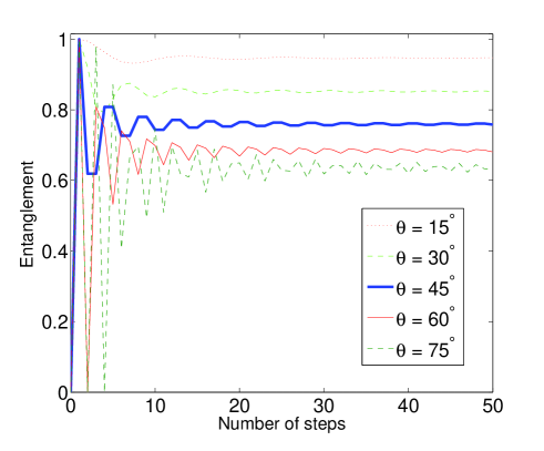
Figure 5: (color online) Entanglement of a single particle with position space when subjected to the QW. The initial state of a particle is $\frac{1}{\sqrt{2}}(|0\rangle+i|1\rangle)$ and is evolved in position space using different values for $\theta$ in the quantum coin operation $C_{0,\theta,0}$. The entanglement initially oscillates and approaches an asymptotic value with an increase in the number of steps. For smaller values of $\theta$ the entanglement is higher and decreases with an increase in $\theta$. Initial oscillation is also larger for higher $\theta$.

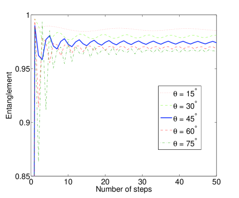
Figure 6: (color online) Entanglement of single particle with position space when subjected to the QW. The initial state of the particle is given by Eq. (2) with $\delta=\frac{2\pi}{9}$ and $\eta=\frac{\pi}{6}$ and is evolved in position space using different values for $\theta$ in the quantum coin operation $C_{0,\theta,0}$. The entanglement initially oscillates and approaches an asymptotic value with an increase in the number of steps. For smaller values of $\theta$ the entanglement is higher and decreases with an increase in $\theta$. Initial oscillation is also larger for higher $\theta$.

Fig. 5 shows a plot of the entanglement against the number of steps of the QW on a particle initially in a symmetric superposition state using different values for $\theta$ in the operation $W_{\theta}$. The von Neumann entropy of the reduced density matrix of the coin is used to quantify entanglement between the coin and the position in Fig. 5. That is,

$$E_{c}(t)=-\sum_{j}\lambda_{j}\rm{log}_{2}(\lambda_{j})$$ (12)

where $\lambda_{j}$ are eigenvalues of the reduced density matrix of the coin after $t$ steps (time). The entanglement initially oscillates and reaches an asymptotic value with increasing number of steps. In the asymptotic limit, the entanglement value decreases with an increase in $\theta$ and this dependence can be attributed to the spread of the amplitude distribution in position space. That is, with an increase in $\theta$, constructive interference of quantum amplitudes toward the origin becomes prominent narrowing the distribution in the position space. In Fig. 6, the process is repeated for a particle initially in an asymmetric superposition state $|\Psi_{in}\rangle=\left[\cos(\frac{2\pi}{9})|0\rangle+e^{i\frac{\pi}{6}}\sin(\frac{2\pi}{9})|1\rangle\right]\otimes|\psi_{0}\rangle$. Comparing Fig. 6 with Fig. 5, we can note the increase in entanglement and decrease in the oscillation. This observation can be explained by going back to our earlier note on biased QW in Sec. II.1. In Fig. 2 we note that biasing of the coin operation leads to an asymmetry in the probability distribution, with an increase in peak height on one side and a decrease on the other side (increase and decrease are in reference to the symmetric distribution). A similar biasing effect can also be reproduced by choosing an asymmetric initial state of the particle. The biased distribution with an increased value of probability at one side in the distribution contributes to a reduced oscillation in the distribution. This in turn results in the increase of the von Neumann entropy: entanglement.

III.2 Spatial entanglement

Spatial entanglement is the entanglement between the lattice points. This entanglement takes the form of non-local particle number correlations between spatial modes. To observe spatial entanglement we first need to associate the lattice with the state of a particle. Then we need to consider the evolution of a single-particle QW followed by the evolution of a many-particle QW, in order to understand spatial entanglement.

III.2.1 Using a single-particle quantum walk

In a single-particle QW, each lattice point is associated with a Hilbert space spanned by two subspaces. The first is the zero-particle subspace which does not involve any coin (particle) states. The other is the one-particle subspace spanned by the two possible states of the coin, $|0\rangle$ and $|1\rangle$. To obtain the spatial entanglement we will write the state of the particle in the form of the state of a lattice. Following from Eq. (11), the state of the particles after first two steps of QW takes the form

$$|\Psi_{2}\rangle = W_{0,\theta,0}|\Psi_{1}\rangle=\gamma\left[\cos(\theta)|0\rangle|\psi_{j-2}\rangle+\sin(\theta)|1\rangle|\psi_{j}\rangle\right]+\delta\left[\sin(\theta)|0\rangle|\psi_{j}\rangle-\cos(\theta)|1\rangle|\psi_{j+2}\rangle\right].$$ (13)

In order to obtain the state of the lattice we can redefine the position state in the following way: the occupied position state $|\psi_{j}\rangle$ as $|1_{j}\rangle$, which means that the $j^{th}$ position is occupied and the rest of the lattice is empty. Therefore, we can rewrite Eq. (13) as

$$|\Psi_{2}\rangle = \gamma\left[\cos(\theta)|0\rangle|1_{j-2}\rangle+\sin(\theta)|1\rangle|1_{j}\rangle\right]+\delta\left[\sin(\theta)|0\rangle|1_{j}\rangle-\cos(\theta)|1\rangle|1_{j+2}\rangle\right].$$ (14)

Since we are interested in the spatial entanglement, we project this state into one of the coin state so that we can ignore the entanglement between the coin and the position state and consider only the lattice states. Here we will choose the coin state to be $|0\rangle$ and take projection to obtain the state of the lattice in the form

$$|\Psi_{lat}\rangle=|0\rangle\left(\gamma\cos(\theta)|1_{j-2}\rangle+\delta\sin(\theta)|1_{j}\rangle\right).$$ (15)

Each lattice site $j$ can be considered as a Hilbert space with basis states $|1_{j}\rangle$ (occupied state) and $|0_{j}\rangle$ (unoccupied state). Then, the above Eq. (15) in the extended Hilbert space of each lattice can be rewritten in terms of occupied and unoccupied lattice states as

$$|\Psi_{lat}^{\prime}\rangle=\gamma\cos(\theta)|1_{j-2}\,0_{j}\rangle+\delta\sin(\theta)|0_{j-2}\,1_{j}\rangle.$$ (16)

We can see that after first two steps of the QW the lattice points $j$ and $(j-2)$ are entangled. One can check that the lattice points $j$ and $(j+2)$ are entangled if we choose the coin state to be $|1\rangle$. With an increase in the number of steps, the state of the particle spreads in position space and the projection over one of the coin state reduces that state to a pure state, for which one may compute spatial entanglement, according to the above prescription. Therefore, with an increase in the number of steps, the spatial entanglement from a single-particle QW decreases.

III.2.2 Using many-particle quantum walk

We will extend the study of evolution of spatial entanglement as the QW progresses on a many-particle system.

Let us first consider the analysis of first two steps of the Hadamard walk ($\theta=\pi/4$ in Eq. (10)) on a three-particle system with the initial state:

$$|\Psi_{ins}^{3p}\rangle=\bigotimes_{j=-1}^{+1}\left(\frac{|0\rangle+i|1\rangle}{\sqrt{2}}\right)\otimes|\psi_{j}\rangle.$$ (17)

We will label the three particles at positions $-1$, $0$ and $1$ as ${\rm A}$, ${\rm B}$ and ${\rm C}$, respectively. Since evolution of these particles is independent, we write down the state after the first step as a tensor product of each of the three particles:

$$|\Psi^{3p}_{1}\rangle=W_{0,\theta,0}^{\otimes 3}|\Psi_{ins}^{3p}\rangle=\left[\gamma|0\rangle|-2\rangle+\delta|1\rangle|0\rangle\right]_{\rm A}\otimes\left[\gamma|0\rangle|-1\rangle+\delta|1\rangle|+1\rangle\right]_{\rm B}\otimes\left[\gamma|0\rangle|0\rangle+\delta|1\rangle|+2\rangle\right]_{\rm C},$$ (18)

where $\gamma=(1+i)/2$ and $\delta=(1-i)/2$. After two steps the tensor product of each of the three particles is given by

$$|\Psi^{3p}_{2}\rangle =\left[\gamma\left(\frac{|0\rangle|-3\rangle+|1\rangle|-1\rangle}{\sqrt{2}}\right)+\delta\left(\frac{|0\rangle|-1\rangle-|1\rangle|+1\rangle}{\sqrt{2}}\right)\right]_{\rm A}$$

$$\otimes\left[\gamma\left(\frac{|0\rangle|-2\rangle+|1\rangle|0\rangle}{\sqrt{2}}\right)+\delta\left(\frac{|0\rangle|0\rangle-|1\rangle|+2\rangle}{\sqrt{2}}\right)\right]_{\rm B}$$

$$\otimes\left[\gamma\left(\frac{|0\rangle|-1\rangle+|1\rangle|+1\rangle}{\sqrt{2}}\right)+\delta\left(\frac{|0\rangle|+1\rangle-|1\rangle|+3\rangle}{\sqrt{2}}\right)\right]_{\rm C}.$$ (19)

By projecting this state into one of the coin states (we choose state $|0\rangle\otimes|0\rangle\otimes|0\rangle$) we can obtain a state of the lattice for which spatial entanglement may be computed. Then the state of the lattice after projection and normalization is

$$|\Psi_{lat}\rangle= \gamma^{3}\,|{\rm A}\rangle_{-3}|{\rm B}\rangle_{-2}|{\rm C}\rangle_{-1}$$

$$+\gamma^{2}\delta\left(\,|{\rm A}\rangle_{-3}|{\rm B}\rangle_{-2}|{\rm C}\rangle_{1}+|{\rm A}\rangle_{-3}|{\rm B}\rangle_{0}|{\rm C}\rangle_{-1}+|{\rm AC}\rangle_{-1}|{\rm B}\rangle_{-2}\right)$$

$$+\gamma\delta^{2}\left(\,|{\rm A}\rangle_{-3}|{\rm B}\rangle_{0}|{\rm C}\rangle_{1}+|{\rm AC}\rangle_{-1}|{\rm B}\rangle_{0}+|{\rm A}\rangle_{-1}|{\rm B}\rangle_{-2}|{\rm C}\rangle_{1}\right)$$

$$+\delta^{3}\,|{\rm A}\rangle_{-1}|{\rm B}\rangle_{0}|{\rm C}\rangle_{1},$$ (20)

where $A,B$ and $C$ represent the particle labels and the subscripts represent the position labels. In a similar manner we can obtain $|\Psi_{lat}\rangle$ for a system with a large number of particles. Then the next task is to calculate the spatial entanglement.

IV Calculating spatial entanglement in a multipartite system

In a system with two particles, the state is separable if we can write it as a tensor product of individual particle states, and entangled if not. For a system with $M>2$ particles, a state is said to be fully separable if it can be written as

$$|\psi\rangle=|\phi_{1}\rangle\otimes|\phi_{2}\rangle\otimes\cdots|\phi_{k}\rangle,$$ (21)

when $k=M$. $|\phi_{i}\rangle$ will then denote the state of the $i^{th}$ particle. When $k<M$ a state is said to be partially entangled and when $k=1$ the state will be fully entangled.

Rather than using the von Neumann entropy to quantify multipartite entanglement of a given state $\rho$, one sometimes often prefers to consider purity, which corresponds (up to a constant) to linear entropy, that is the first-order term in the expansion of the von Neumann entropy around its maxima, given by

$$E=\frac{d}{d-1}\left[1-{\rm Tr}\rho^{2}\right]$$ (22)

for a $d$-dimensional particle Hilbert space PWK04 . To quantify the entanglement of multipartite pure states, one measure commonly, used is the Meyer- Wallach (M-W) measure MW02 . It is the entanglement measure of a single particle to the rest of the system, averaged over the whole of the system and is given by

$$E_{MW}=\frac{d}{d-1}\left[1-\frac{1}{L}\sum_{i=1}^{L}{\rm Tr}\rho_{i}^{2}\right]$$ (23)

where $L$ is the system size and $\rho_{i}$ is the reduced density matrix of the $i^{th}$ subsystem. The M-W measure does not diverge with increasing system size and is relatively easy to calculate.

In a multipartite QW the dimension at each lattice point, after projection over one particular state of coin, is $2^{M}$ where $M$ is the number of particles. Hence, the expression for entanglement will be

$$E_{MW}(|\psi_{lat}\rangle) =\frac{2^{M}}{2^{M}-1}\left(1-\frac{1}{2t+M+1}\sum_{j=-(t+\frac{M}{2})}^{t+\frac{M}{2}}{\rm tr}\rho_{j}^{2}\right)$$ (24)

where $t$ is the number of steps and $\rho_{j}$ is the reduced density matrix of $j^{th}$ lattice point. The reduced density matrix $\rho_{j}$ can be written as

$$\rho_{j} =\sum_{k}p^{j}_{k}|k\rangle\langle k|$$ (25)

where $|k\rangle$ is one of the $2^{M}$ possible states available for a lattice point and $p^{j}_{k}$ can be calculated once we have the probability distribution of an individual particle on the lattice.

Since we have $M$ distinguishable particles, we have $2^{M}$ configurations depending upon whether a given particle is present in the lattice point or not after freezing the state of the particle. This set of configurations forms the basis for a single-lattice point Hilbert space. Now we can calculate $p^{j}_{k}$, the probability of $k^{th}$ configuration of a particle in the $j^{th}$ lattice point as follows. Let us say $a_{j}^{(l_{i})}$ is the probability of the $i^{th}$ particle to be or not to be in the $j^{th}$ lattice point depending on $l_{i}$. If $l_{i}$ is $1$, then it gives us the probability of the particle to be in the lattice point. If $l_{i}$ is $0$, then $a^{(l_{i})}_{j}$ is the probability of a particle not to be in the lattice point, that is, $a_{j}^{(0)}=1-a_{j}^{(1)}$. Hence, we can write

$$p^{j}_{k} =\prod_{i}a^{l_{i}}_{j}.$$ (26)

Once we have the probability of each particle at a given lattice position, the spatial entanglement can be conveniently calculated. Since the QW is a controlled evolution, one can obtain a probability distribution of each particle over all lattice positions. In fact, one can easily control the probability distribution by varying quantum coin parameters during the QW process and hence the entanglement.

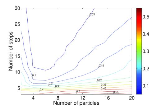
Figure 7: (color online) Evolution of spatial entanglement with an increase in the number of steps of the QW for different number of particles in an open one-dimensional lattice chain. The entanglement first increases and with further increase in the number of steps, the number of lattice positions exceeds the number of particles in the system resulting in the decrease of the spatial entanglement. The distribution is obtained by implementing the QW on particles in the initial state $\frac{1}{\sqrt{2}}(|0\rangle+i|1\rangle)$ and the Hadamard operation $C_{0,\pi/4,0}$ as quantum coin operation.

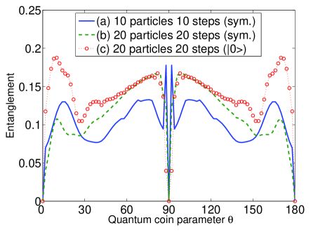
Figure 8: (color online) Quantity of spatial entanglement for 10 particles after 10 steps and 20 particles after 20 steps of the QW on a one-dimensional lattice using different values of $\theta$ in the quantum coin operation $C_{0,\theta,0}$. For (a) and (b), the distribution is for particles initially in the symmetric superposition state, $\frac{1}{\sqrt{2}}(|0\rangle+i|1\rangle)$, and for (c) the particle’s initial state is $|0\rangle$ (will be the same for state $|1\rangle$). Quantity of entanglement is higher for $\theta$ closer to $0$ and $\pi/2$ compared to the intermediate value. We note that the asymmetric probability distribution due to an asymmetric initial state in case of (c) contributes for an increase in the quantity of spatial entanglement. When $\theta=\pi/2$, for every even number of steps of the QW, the system returns to the initial state where entanglement is $0$. Entanglement is 0 for $\theta=0$.

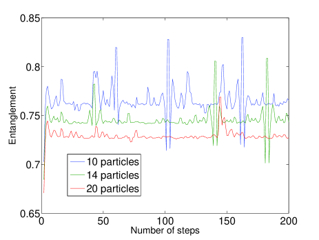
Figure 9: (color online) Evolution of spatial entanglement for a system with different number of particles in a closed chain. With an increase in the number of steps, the entanglement value remains close to asymptotic value with some peaks in between. The peaks can be accounted for the crossover of leftward and rightward propagating amplitudes of the internal state of the particle during the QW. The peaks are more for a chain with a smaller number of particles. An increase in the number of particles in the system results in the decrease of the entanglement value. The distribution is obtained by using $\frac{1}{\sqrt{2}}(|0\rangle+i|1\rangle)$ as the initial states of all particles and the Hadamard operation $C_{0,\pi/4,0}$ as quantum coin operation.

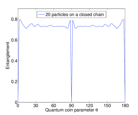
Figure 10: (color online) Quantity of spatial entanglement for 20 particles on a closed chain after 20 steps of the QW using different values of $\theta$ in the quantum coin operation $C_{0,\theta,0}$. The distribution is for particles initially in the state $\frac{1}{\sqrt{2}}(|0\rangle+i|1\rangle)$. Since the system is a closed chain, the QW does not expand the position Hilbert space, and therefore for all values of $\theta$ from $0$ to $\pi/2$ the entanglement value remains roughly uniform except for a small peak at smaller values of $\theta$. For $\theta=0$ when the number of steps equal to the number of particles, the amplitudes goes round the chain and returns to its initial state making the entanglement $0$ and for $\theta=\pi/2$, for every even number of steps of the QW, the system returns to the initial state where entanglement is again $0$.

Fig. 7 shows the phase diagram of the spatial entanglement using a many-particle QW. Data for the phase diagram were obtained numerically by subjecting the many-particle system with different number of particles to the QW with increasing number of steps. The quantity of spatial entanglement was computed using Eq. (24).

Here, we have chosen the Hadamard operation $C_{0,\pi/4,0}$ and $\frac{1}{\sqrt{2}}(|0\rangle+i|1\rangle)$ as the quantum coin operation and initial state of the particles, respectively, for the evolution of the many-particle QW. To see the variation of entanglement for a fixed number of particles with an increase in steps, we can pick a line parallel to the $y$ axis. That is, fix the number of particles and see the variation of entanglement with the number of steps.

In Fig. 7, we see that for a fixed number of particles, the entanglement at first increases to some value before gradually falling. For $M=12$ we can note that the peak value is about $0.5$ before gradually falling. With an increase in the number of steps of the QW, the number of lattice positions to which the particles evolve increases resulting in the decrease of the spatial entanglement (see Eq. (24)). The decrease in entanglement before the number of steps is equal to the number of particles should be noted. This is because for the Hadamard walk the spread of a probability distribution after $t$ steps is between $\frac{-t}{\sqrt{2}}$ and $\frac{t}{\sqrt{2}}$ CSL08 .

If we fix the number of steps and measure the entanglement by increasing the number of particles in the system, the quantity of spatial entanglement first decreases and then it starts increasing with an increase in the number of particles.

To show the variation of spatial entanglement with the quantum coin parameter $\theta$, we plot the spatial entanglement by varying the parameter $\theta$ for a system with 10 particles after 10 steps of the QW and for a system with 20 particles after 20 steps of the QW in Fig. 8. In this figure, (a) and (b) are plots that use the symmetric superposition state $\frac{1}{\sqrt{2}}(|0\rangle+i|1\rangle)$ (unbiased QW) as an initial state of all the particles, and (c) is the plot with all the particles in one of the basis states $|0\rangle$ or $|1\rangle$ (biased QW) as the initial state. We note that the quantity of entanglement is higher for $\theta$ values closer to $0$ and $\pi/2$ and dips for values in between for all the three cases. Biasing the QW, plot (c) shows a slight increase in the quantity of entanglement compared to the unbiased case, plot (b). A similar effect is seen by biasing the QW using two parameters $\xi,\zeta$ in the coin operation $C_{\xi,\theta,\zeta}$ on particles initially in a symmetric superposition state.

Closed chain: Since most physical systems considered for implementation will be of a definite dimension, we extend our calculations to one of the simplest examples of closed geometry, an $n-$cycle. For a QW on an $n-$cycle, the shift operation, Eq. (4), takes the form

$$S=|0\rangle\langle 0|\otimes\sum_{j=0}^{n-1}|\psi_{j-1\mbox{~{}mod~{}}n}\rangle\langle\psi_{j}|+|1\rangle\langle 1|\otimes\sum_{j=0}^{n-1}|\psi_{j+1\mbox{~{}mod~{}}n}\rangle\langle\psi_{j}|.$$ (27)

When we consider a many-particle system in a closed chain, with the number of lattice positions equal to the number of particles $M$, the QW process does not expand the position Hilbert space like it does on an open chain (line). Therefore the spatial entanglement does not decrease at later times as it does for a walk on an open chain, but remains close to the asymptotic value. Fig. 9 shows the evolution of entanglement for a system with different number of particles in a closed chain. The peaks seen in the plot can be accounted for by the crossover of the leftward and rightward propagating amplitudes of the internal state of the particle during the QW process. The frequency of the peaks is more for a smaller number of particles (smaller closed chain). Also, note that the increase in the number of particles and the number of lattice points in the closed cycle results in the decrease in spatial entanglement of the system.

In Fig. 10, the value of spatial entanglement for 20 particles on a closed chain after 20 steps of the QW using different values of $\theta$ in the quantum coin operation $C_{0,\theta,0}$ is presented. For all values of $\theta$ from $0$ to $\pi/2$ the entanglement value remains roughly uniform except for the extreme values of $\theta$. For $\theta=0$, the amplitude goes round the ring and returns to its initial state making the spatial entanglement value $=0$. For $\theta=\pi/2$, for every even number of steps of the QW, the system returns to the initial state where spatial entanglement is again $0$.

Therefore, spatial entanglement on a large lattice space can be created, controlled and optimized for a maximum entanglement value by varying the quantum coin parameters and number of particles in the multi-particle QW.

V Conclusion

We have presented the evolution of spatial entanglement in a many-particles system subjected to a QW process. By considering many particle in the one-dimensional open and closed chain we have shown that spatial entanglement can be generated and controlled by varying the quantum coin parameters, the initial state and the number of steps in the dynamics of the QW process. The spatial entanglement generated can have a potential application in quantum information theory and other physical processes.

Acknowledgement

C.M.C is thankful to Mike and Ophelia Lezaridis for the financial support at IQC, ARO, QuantumWorks and CIFAR for travel support. C.M.C also thank IMSc, Chennai, India for the hospitality during November - December 2008. S.K.G thanks Aiswarya Cyriac for the help in programming.

References

- (1) Michael Nielsen and Issac Chuang, Quantum Computation and Quantum Information, Cambridge University Press, 2000
- (2) Ryszard Horodecki, Pawel Horodecki, Michal Horodecki, and Karol Horodecki, Rev. Mod. Phys. 81, No. 2, 865-942 (2009).
- (3) T. J. Osborne and M. A. Nielsen, Phys. Rev. A 66, 032110 (2002).
- (4) A. Osterloh, L. Amico, G. Falci, and R. Fazio, Nature (London) 416, 608 (2002).
- (5) T. R. de Oliveria, G. Rigolin, M. C. de Oliveria, and E. Miranda, Phys. Rev. Lett. 97, 170401 (2006).
- (6) S. Bose and D. Home, Phys. Rev. Lett. 88, 050401 (2002).
- (7) M. S. Leifer, L. Henderson, and N. Linden, Phys. Rev. A 67, 012306 (2003).
- (8) O. Romero-Isart, K. Eckert, C. Rod , and A Sanpera, J. Phys. A: Math. Theor. 40, 8019-8031(2007).
- (9) Xiaoting Wang and S. G. Schirmer, Phys. Rev. A 80, 042305 (2009).
- (10) L. Amico, R. Fazio, A. Osterloh, and V. Vedral, Rev. Mod. Phys. 80, 517, (2008).
- (11) Julia Kempe, Contemporary Physics 44, 307 327 (2003).
- (12) Ivens Carneiro, Meng Loo, Xibai Xu, Mathieu Girerd, Viv Kendon and Peter L. Knight, New J. Phys. 7, 156 (2005).
- (13) A. Ambainis, Int. Journal of Quantum Information, 1, No. 4, 507-518 (2003).
- (14) C. M. Chandrashekar and R. Laflamme, Phys. Rev. A 78, 022314 (2008).
- (15) Takashi Oka, Norio Konno, Ryotaro Arita, and Hideo Aoki, Phys. Rev. Lett. 94, 100602 (2005).
- (16) Gregory S. Engel et. al., Nature, 446, 782-786 (2007).
- (17) M. Mohseni, P. Rebentrost, S. Lloyd, and A. Aspuru-Guzik, j. Chem. Phys. 129, 174106 (2008).
- (18) Jiangfeng Du, Hui Li, Xiaodong Xu, Mingjun Shi, Jihui Wu, Xianyi Zhou, and Rongdian Han, Phys. Rev. A 67, 042316 (2003)
- (19) C.A. Ryan, M. Laforest, J.C. Boileau, and R. Laflamme, Phys. Rev. A 72, 062317 (2005).
- (20) H.B. Perets, Y. Lahini, F. Pozzi, M. Sorel, R. Morandotti, and Y. Silberberg, Phys. Rev. Lett. 100, 170506 (2008).
- (21) K. Karski, L. Foster, J.-M. Choi, A. Steffen, W. Alt, D. Meschede, and A. Widera, Science, 325, 174 (2009).
- (22) B.C. Travaglione and G.J. Milburn, Phys. Rev. A 65, 032310 (2002).
- (23) W. Dur, R. Raussendorf, V. M. Kendon, and H.J. Briegel, Phys. Rev. A 66, 052319 (2002).
- (24) K. Eckert, J. Mompart, G. Birkl, and M. Lewenstein, Phys. Rev. A 72, 012327 (2005).
- (25) C. M. Chandrashekar, Phys. Rev. A 74, 032307 (2006).
- (26) Z.-Y. Ma, K. Burnett, M. B. d’Arcy, and S. A. Gardiner, Phys. Rev. A 73, 013401 (2006).
- (27) G. V. Riazanov, Sov. Phys. JETP 6, 1107 (1958).
- (28) R. P. Feynman and A. R. Hibbs, Quantum Mechanics and Path Integrals (McGraw-Hill, New York, 1965).
- (29) Y. Aharonov, L. Davidovich and N. Zagury, Phys. Rev. A 48, 1687, (1993).
- (30) David A. Meyer, J. Stat. Phys. 85, 551 (1996).
- (31) A. Ambainis, E. Bach, A. Nayak, A. Vishwanath, and J. Watrous, Proceeding of the 33rd ACM Symposium on Theory of Computing (ACM Press, New York), 60 (2001).
- (32) E. Farhi and S. Gutmann, Phys.Rev. A 58, 915 (1998).
- (33) Fredrick Strauch, Phys. Rev. A 74, 030310 (2006).
- (34) C. M. Chandrashekar, Phys. Rev. A 78, 052309 (2008).
- (35) A. Ambainis, J. Kempe and A. Rivosh, Proceedings of ACM-SIAM Symposium on Discrete Algorithms (SODA), (AMC Press, New York), 1099-1108, (2005).
- (36) C. M. Chandrashekar, R. Srikanth, and R. Laflamme, Phys. Rev. A 77, 032326 (2008).
- (37) Valerie Coffman, Joydip Kundu, and William K. Wootters, Phys. Rev. A 61, 052306 (2000).
- (38) H. Barnum and N. Linden, Monotones and Invariants for Multi-particle Quantum States, J. Phys. A: Math. Gen. 34, 6787 (2001).
- (39) Jens Eisert and Hans J. Briegel, Phys. Rev. A 64, 022306 (2001).
- (40) D. A. Meyer and N. R. Wallach, J. Math. Phys. 43, 4273 (2002).
- (41) Frank Verstraete, Jeroen Dehaene, and Bart De Moor, Phys. Rev. A 68, 012103 (2003).
- (42) Akimasa Miyake, Phys. Rev. A 67, 012108 (2003).
- (43) Ali Saif M. Hassan and Pramod S. Joag, Phys. Rev. A 77, 062334 (2008).
- (44) L. Heaney, J. Anders, D. Kaszlikowski and V. Vedral, Phys. Rev. A 76, 053605 (2007).
- (45) Kathy-Anne Brickman Soderberg, Nathan Gemelke, and Cheng Chin, New Journal of Physics 11, 055022 (2009).
- (46) Sougato Bose, Phys. Rev. Lett., 91, 207901 (2003).
- (47) Matthias Christandl, Nilanjana Datta, Artur Ekert, and Andrew J. Landahl, Phys. Rev. Lett. 92, 187902 (2004)
- (48) Matthias Christandl, Nilanjana Datta, Tony C. Dorlas, Artur Ekert, Alastair Kay, and Andrew J. Landahl, Phys. Rev. A 71, 032312 (2005).
- (49) Nicholas A. Peters, Tzu-Chieh Wei, and Paul G. Kwiat , Phys. Rev. A 70 052309 (2004).