Excised black hole spacetimes: quasi-local horizon formalism applied to the Kerr example

Abstract

We present a numerical work aiming at the computation of excised initial data for black hole spacetimes in full general relativity, using Dirac gauge in the context of a constrained formalism for the Einstein equations. Introducing the isolated horizon formalism for black hole excision, we especially solve the conformal metric part of the equations, and assess the boundary condition problem for it. In the stationary single black hole case, we present and justify a no-boundary treatment on the black hole horizon. We compare the data obtained with the well-known analytic Kerr solution in Kerr-Schild coordinates, and assess the widely used conformally flat approximation for simulating axisymmetric black hole spacetimes. Our method shows good concordance on physical and geometrical issues, with the particular application of the isolated horizon multipolar analysis to confirm that the solution obtained is indeed the Kerr spacetime. Finally, we discuss a previous suggestion in the literature for the boundary conditions for the conformal geometry on the horizon.

I Introduction

Trying to accurately describe black holes solutions as evolving physical objects in numerical simulations is of direct interest in astrophysics. Numerical simulations have made a great leap forward in the past few years, mainly with the first stable simulations of black hole mergers in full general relativity by Pretorius Pret05 , Campanelli et al. Camp , Baker et al. BC06 , and a few other groups (see Pret07 for a review). Several of these simulations model black holes in their equations by punctures. These punctures basically change the topology of spacetime to handle evolution of singular objects (see BrBr for the first proposal of this method).

Notable exceptions to this are references Pret05 ; Caltech ; SziPolRez07 ; Spe07 , that use an excision approach for black hole evolution: the simulations only evolve the spacetime outside two-spheres that are supposed to encircle the black hole singularities.

In the same spirit, we are here trying to describe black holes as physical objects characterized by their horizons. Defining the physical laws for event horizons of black holes has been notably done by HawHar , Dam79 and TPM86 in a so-called membrane paradigm. The aim was to describe them as fluid-like two-membranes with physical properties. However, applying evolution laws to event horizons is problematic due to their teleological (non causal) behavior (see for example Boo05 for a description of the phenomenon). Being defined as a global property of spacetime, a local notion of causality actually does not apply to event horizons.

Alternative local characterizations have been formulated in the past 15 years by Hay94 , AshBF and AshKr03 . They are based on the concept of trapped surfaces, dating back to Penrose’s singularity theorem Pen65 . Defined locally, those objects behave in a causal way in a general dynamical context, with local evolution laws following from the projection of Einstein equations, e.g the Navier-Stokes Gourg05 “fluid bubble” analogy or the area evolution law in GouJar06b . For this work we shall use local characterizations for isolated horizons, prescribing the physics of non-evolving black hole horizons.

Following the prescriptions of Cook02 , GJM04 , GJ06 and pursuing the numerical explorations of CookPf04 ; CauCooGri06 and JAL07 among others, we try to numerically implement those objects as boundary conditions imposed on the (3+1) form of Einstein equations, in a three-slice excised by a two-surface (single black hole case). This is done here using the fully constrained formalism (FCF) of Bon04 (see also Cord1 ), with maximal slicing and Dirac gauge, based on the (3+1) formalism, and with spectral methods-based numerical resolution using the LORENE library LORENE . An important point here is that we drop out the usual conformal flatness hypothesis and solve for the conformal geometry, so that we can exactly recover a slice of a stationary rotating vacuum spacetime.

Contrary to free evolution schemes, which are the most used prescription for (3+1) simulations in numerical relativity, an important feature of constrained schemes is the necessity to solve constraints on each three-slice, in the form of elliptic equations. These equations generally need additional conditions to be imposed on grid boundaries, following reasonable geometrical and physical prescriptions. Our approach particularly requires a specific handling of boundary conditions for the two dynamical gravitational degrees of freedom. This is a crucial point of our calculation; we will justify and apply here a no-boundary treatment for these quantities.

The paper is organized as follows: we first review in Sec. II fundamental geometrical properties associated with isolated horizons in general relativity. In Sec.  III, we quickly give the basic features of the fully constrained formalism and the methods we use to treat the conformal part. Sec. IV discusses implementation of boundary conditions for the system of equations, and specifically discusses the conformal metric part. Sec. V gives the numerical results obtained, and confronts them to a battery of tests characterizing the physics of the solutions. A discussion follows in Sec. VI, in regard of previous works concerning the computation of the conformal part in the black hole initial data problem. We also raise the question of applicability of this scheme to other more general astrophysical cases.

Throughout all this paper, Greek letters will denote indices spanning from 0 to 3, Latin indices from $k$ to $m$ shall denote indices from $\{1,2,3\}$, and indices from $a$ to $c$ have the range of $\{2,3\}$. All formulae and values are given in geometrical units ($G=c=1$). We also use the Einstein summation convention.

II Isolated horizons as a local description of black hole regions

II.1 Trapped surfaces and expansion

The concept of a trapped surface in a Lorentzian frame has been first defined by Penrose in 1965 Pen65 in connection with the singularity theorems. It relies on the notion of expansion of the light rays emitted from a surface, that we explain here. We start by a closed spacelike two-surface $\mathcal{S}$ embedded in spacetime, topologically related to a two-sphere. We assign to it a two-metric $q_{ab}$ induced by the ambient four-metric $g_{\mu\nu}$, and its associated area form $\epsilon^{\mathcal{S}}_{ab}$. Two future null directions orthogonal to $\mathcal{S}$ are associated with this surface. Representative vector fields are denoted $\ell^{\mu}$ and $k^{\mu}$, being respectively oriented outwards and inwards. We can for example assume that our spacetime is asymptotically flat, so the orientation can be defined without ambiguity.

The expansion $\theta_{\ell}$ of $\mathcal{S}$ along $\ell^{\mu}$ is the area rate of change along this vector: $\mathcal{L}_{\ell}\,{\epsilon}^{\mathcal{S}}_{ab}=\theta_{\ell}\,\epsilon^{\mathcal{S}}_{ab}$. $\mathcal{L}$ is the Lie derivative, here along the vector $\ell^{\mu}$. Same definition goes for the vector field $k^{\mu}$. For a two-sphere embedded in a Minkowski spacetime (flat metric), we have typically $\theta_{k}<0$ and $\theta_{\ell}>0$. $\mathcal{S}$ is said to be a trapped surface if both expansions are negative or zero: $\theta_{\ell}\leq 0$ , $\theta_{k}\leq 0$. This clearly characterizes strong local curvature. A marginally (outer) trapped surface will be characterized by $\theta_{\ell}=0$ and $\theta_{k}\leq 0$. Two theorems make the connection between those objects and black holes: provided the weak energy condition holds, the singularity theorem of Penrose Pen65 ensures that a spacetime containing a trapped surface necessarily contains a singularity in its future. Following this result, provided the cosmic censorship holds, another result by Hawking and Ellis HawEll73 conveys that a spacetime containing a trapped surface necessarily contains a black hole region enclosing this surface.

Marginally outer trapped surfaces (MOTS) are intended as models for the black hole boundary (see Senov08 for a discussion of its relation with the boundary of the black hole trapped region). Local horizons (trapping horizons for Hay94 , isolated and dynamical horizons in AshBF , AshKr03 ) are defined as three-dimensional tubes “sliced” by MOTS, with additional geometrical properties. The isolated horizon case is detailed below; for a review, see AshKr04 .

In vacuum stationary spacetimes, all horizons are at the same location, which is also the location of the event and apparent horizons (constructed with outermost MOTSs). In the more general case, and assuming cosmic censorship, local horizons are always situated inside the event horizon in general relativity.

II.2 Isolated horizons

The notion of isolated horizon is aimed at describing stationary black holes. It is based on the notion of non-expanding horizons, and defined as a three-dimensional tube $\mathcal{H}$ foliated by MOTS, and with a null vector field $\ell^{\mu}$ as generator. The three-metric induced on the tube has then a signature $(0,+,+)$.

We also define a (3+1) spatial slicing for our spacetime, and $\mathcal{S}$ a two-slice of our isolated horizon at a certain value of the time parameter $t$. The spacelike two-metric on $\mathcal{S}$ is denoted $q_{ab}$.

The shear tensor $\sigma_{ab}$ on the two-surface is defined along $\ell^{\mu}$ as

$$\sigma_{ab}=\frac{1}{2}\left[\mathcal{L}_{\ell}\,q_{ab}-\theta_{\ell}q_{ab}\right].$$ (1)

Using the fact that $\theta_{\ell}=0$ and the dominant energy condition, the Raychaudhuri equation for null tubes GJ06 ensures that both the shear along $\ell^{\mu}$ and the energy-momentum tensor projected on $\ell^{\mu}$, and evaluated on the surface must vanish: $\sigma_{ab}=0$ and $T_{ab}\ell^{a}\ell^{b}=0$. These are additional properties constraining the geometry of the horizon.

An isolated horizon is also required to be such that the extrinsic geometry of the tube is not evolving along the null generators: $[\mathcal{L}_{(\ell)},D_{i}^{\cal H}]=0$, where $D_{i}^{\cal H}$ is the connection on the tube induced from the ambient spacetime connection. If this last condition is dropped, we only retrieve a non-expanding horizon (linked to the notion of “perfect horizon” Haj73 ).

The isolated horizon formalism has already been studied extensively in numerics, as a diagnosis for simulations involving black holes, where marginally trapped surfaces are found a posteriori with numerical tools called apparent horizon finders (See for example Thorn , LinNov07 , AHfinder1 , AHfinder2 ). Let us note that very often, apparent horizon finders actually locate MOTS on the three-slice considered (not necessarily outermost ones). A thorough study of geometrical properties of isolated horizons located a posteriori can be found in DrKrSch03 .

In the present paper we employ isolated horizons as an a priori ingredient in the numerical construction of Cauchy initial data for black hole spacetimes. More precisely, we impose conditions on the excised surface characterizing it as the slice of a non-expanding horizon (see below). This approach to the modeling a black hole horizon in instantaneous equilibrium has been investigated in Cook02 ; CookPf04 ; CauCooGri06 ; GJM04 ; DaiJarKri05 ; GJ06 ; JAL07 , where a prescription for the conformal metric is assumed. The main feature of this work is the inclusion of the conformal metric in the discussion, not through analytical prescriptions, but indeed by numerical calculation. This problem has also been recently addressed in CookBaum08 . In Sec. IV we tackle the description of our special treatment of the conformal metric on the excised boundary and compare with previous results, in particular through the numerical recovery of excised Kerr initial data.

III A fully constrained formalism for Einstein equations

All the following is a summary of the physical and technical assumptions set in Bon04 . For a review of (3+1) formalism in numerical relativity, the reader is referred to York79 , or more recent reviews like Gourg07 and Alc08 .

III.1 Notations and (3+1) decomposition

We consider an asymptotically flat, globally hyperbolic four-dimensional manifold $\mathcal{M}$, associated with a metric $g_{\mu\nu}$ of Lorentzian signature $(-,+,+,+)$. We define on $\mathcal{M}$ a slicing by spacelike hypersurfaces $\Sigma_{t}$, labeled by a timelike scalar field $t$; in this way, the four-metric can be written in its usual (3+1) form:

$$g_{\mu\nu}dx^{\mu}dx^{\nu}=-N^{2}dt^{2}+\gamma_{ij}(dx^{i}+\beta^{i}dt)(dx^{j}+\beta^{j}dt),$$ (2)

here $N$ and $\beta^{i}$ are the usual lapse scalar field and shift vector field. $\gamma^{ij}$ is the spacelike three-metric induced on $\Sigma_{t}$.

We also define the second fundamental form of $\Sigma_{t}$, or extrinsic curvature tensor, as:

$$K_{\mu\nu}=-\frac{1}{2}{\mathcal{L}_{n}}\gamma_{\mu\nu},$$ (3)

with $n^{\mu}$ the future-directed vector field normal to $\Sigma_{t}$. Writing the vacuum Einstein equations with this formalism, one comes up with the classical (3+1) vacuum Einstein equations system(see for example ADM62 ):

$$R+K^{2}-K_{ij}K^{ij} = 0,$$ (4)

$$D_{j}K_{i}^{j}-D_{i}K = 0,$$ (5)

$$\frac{\partial}{\partial t}K_{ij}-{\mathcal{L}}_{\beta}K_{ij} =$$

$$-D_{i}D_{j}N + N\left\{R_{ij}-2K_{ik}K^{k}_{j}+KK_{ij}\right\},$$ (6)

$D_{i}$ and $R_{ij}$ being, respectively, the connection and the Ricci tensor associated with the three-metric $\gamma_{ij}$. Quantities without indices represent tensorial traces. These equations are referred to respectively as the Hamiltonian constraint, momentum constraint and evolution equations.

III.2 Conformal decomposition, maximal slicing and Dirac gauge

Now we must choose a set of variables and a gauge, to get a partial differential equations system that we solve numerically. The first ingredient in the formalism presented in Bon04 is the conformal decomposition of the three-metric Lichn42 . We define on each slice $\Sigma_{t}$ an extra metric noted $f_{ij}$, that will have a vanishing Riemann tensor (flat metric) and will be time independent. The existence of such a metric in a neighborhood of spatial infinity is ensured by our sub-manifold being asymptotically flat. The associated flat connection is noted $\mathcal{D}_{i}$. We introduce in $\Sigma_{t}$ a conformal metric such that its determinant coincides with that of $f_{ij}$, as:

$$\tilde{\gamma}_{ij}=\psi^{-4}\gamma_{ij};\quad\psi=\left(\frac{\textrm{det}(\gamma)}{\textrm{det}(f)}\right)^{\frac{1}{12}}.$$ (7)

The tensor field $h^{ij}$ we use to encode the conformal degrees of freedom is the deviation of the conformal metric from the flat one:

$$\tilde{\gamma}^{ij}=f^{ij}+h^{ij}.$$ (8)

We also define in our equation sources the following conformal traceless extrinsic curvature:

$$\hat{A}^{ij}=\psi^{10}(K^{ij}-\frac{1}{3}K\gamma^{ij});$$ (9)

We choose for a gauge the generalized Dirac gauge for the conformal metric:

$${\mathcal{D}}_{k}\tilde{\gamma}^{ki}={\mathcal{D}}_{k}h^{ki}=0,$$ (10)

and we add to this prescription the maximal slicing condition, i.e the vanishing of the trace in the extrinsic curvature: $K=0$. Therefore, $\hat{A}^{ij}$ contains all the information about extrinsic geometry.

Under those conditions, we can rewrite the (3+1) Einstein equations in what we shall call the FCF system:

$$\Delta\psi = \mathcal{S}_{\psi}(N,\psi,\beta^{i},\hat{A}^{ij},h^{ij}),$$ (11)

$$\Delta(N\psi) = \mathcal{S}_{(N\psi)}(N,\psi,\beta^{i},\hat{A}^{ij},h^{ij}),$$ (12)

$$\Delta\beta^{i}+\frac{1}{3}\mathcal{D}^{i}\mathcal{D}_{j}\beta^{j} = \mathcal{S}_{\beta}^{i}(N,\psi,\beta^{i},\hat{A}^{ij},h^{ij}),$$ (13)

$$\frac{\partial^{2}h^{ij}}{\partial t^{2}}-\frac{N^{2}}{\psi^{4}}\Delta h^{ij} - 2\mathcal{L}_{\bm{\beta}}\frac{\partial h^{ij}}{\partial t}+\mathcal{L}_{\bm{\beta}}\mathcal{L}_{\bm{\beta}}h^{ij}=$$ (14)

$$\mathcal{S}_{h^{ij}}^{ij}(N,\psi,\beta^{i},\hat{A}^{ij},h^{ij}).$$

$\Delta$ is the usual scalar flat laplacian (which expression from a spectral point of view is recalled in the Appendix A). The actual sources $\mathcal{S}_{\cdots}$, in general non-linear in the variables and time-dependent, can be retrieved by the reader from Bon04 .

We must supplement this system with the kinematical relation between the three-metric and extrinsic curvature of the slice, deduced from (3) and (9) (see equation (92) of Bon04 ). This fully constrained scheme is strictly equivalent to the one presented in Bon04 . A slightly different version has been presented recently in Cord1 , focusing on non-uniqueness issues. Although the scheme in Cord1 would probably pose no additional difficulty in the present setting (except maybe some more boundary conditions to prescribe to additional variables), there has been no significant indication of problems involving non-uniqueness of solutions in our study, that suggested modifications of the original formalism.

Here we choose as variables the quantities $N\psi$, $\psi$, $\beta^{i}$ and $h^{ij}$. We especially come up with three elliptic equations, two scalar and one vectorial. Those are derived directly from the Hamiltonian and momentum constraints of the (3+1) system, together with the trace part of the dynamical equations. In an evolution scheme, these will be the conditions enforced at each value of time $t$. We do this for one particular slice.

We are then left in general with a second-order tensorial hyperbolic equation (14) dealing with the variable $h^{ij}$, that is obtained by the geometrical relation between $\gamma_{ij}$ and $K_{ij}$, and the dynamical part of Einstein equations.

The goal here is to simulate as accurately as possible stationary spacetimes containing one black hole, represented by an isolated horizon. In this respect, we shall assume a coordinate system that is adapted to stationarity. This will mean that a stationary timelike Killing vector field will be identified with our time evolution vector field $(\frac{\partial}{\partial t})^{i}$. Using this prescription, all the time derivatives in our equations vanish, so that our sources and operators simplify somewhat. In particular, the tensorial equation is written using an ellipticlike operator acting on $h^{ij}$:

$$\Delta h^{ij}-\frac{\psi^{4}}{N^{2}}\mathcal{L}_{\beta}\mathcal{L}_{\beta}h^{ij}=\mathcal{S}_{2}^{ij}(h^{ij},N,\psi,\beta,A^{ij}).$$ (15)

Our problem is then totally equivalent to an actual initial data problem, where quantities have to be determined on a three-slice by elliptic equations, before evolving them. The main difference with classical initial data schemes like the conformal transverse traceless (CTT), the extended conformal thin sandwich (XCTS) scheme or the conformal flat curvature (CFC) system, is an additional elliptic equation for the conformal geometry of the three-slice. Up to now, a vast majority of initial data computations have been done using an ad hoc prescription for the conformal geometry. The most common one is the conformally flat approach, where $\tilde{\gamma_{ij}}$ is simply approximated to be the 3D flat metric. This has been done in numerous computations, and this type of initial data is the most frequently used for black hole evolution simulations. However, though this conformally flat approximation turns out to be well-behaved in most cases, we know that it is a strong limitation when trying to compute stationary black hole spacetimes: it has been proven that the rotating Kerr-Newman spacetime does not admit any conformally flat slice (see Val04b ; Dainn ).

Other prescriptions for the conformal geometry include data suggested by the post-Newtonian formalism PN , or superposition of additional gravitational wave content (see BSeid96 ). Let us mention the work of ShibLim for neutron-star binary initial data, which also computes the conformal geometry using a prescription in ShibUrFr , that considers as well the dynamical Einstein equations for the conformal variables. Finally, the exact scheme we have explicated above has been applied by one of the authors in the case of a single rotating neutron star in equilibrium LinNov06 . It has led to the computation of strictly stationary initial data, that can be directly extended into future and past time directions. This is exactly what we are trying to do here in the black hole case.

III.3 Resolution of conformal metric part

Apart from the boundary condition problem (that we discuss in Sec. IV), our approach for the resolution of the tensorial equation presents some peculiarities that we explain here.

The system of equations is composed of equation (15) and the gauge condition:

$$\mathcal{D}_{i}h^{ij}=0,$$ (16)

that we supplement with a condition on the determinant of $\tilde{\gamma}^{ij}$, following from our definition of the conformal factor:

$$\textrm{det}(\tilde{\gamma}^{ij})=\textrm{det}(h^{ij}+f^{ij})=1.$$ (17)

We are left with a tensorial equation for a symmetric tensor with four constraints: the system has two degrees of freedom. We now try to make them explicit and solve for the related variables. Any second-rank symmetric tensor $h^{ij}$ can be decomposed in the following way into a divergence free part, and a symmetrized gradient part:

$$h^{ij}=\mathcal{D}^{i}W^{j}+\mathcal{D}^{j}W^{i}+h^{ij}_{T},$$ (18)

with $\mathcal{D}_{i}h^{ij}_{T}=0$. We shall use here variables associated only with the divergence-free part $h^{ij}_{T}$, meaning that the gauge component (gradient part) of the tensor considered has no influence on them. We choose to encode the information in $h^{ij}_{T}$ in the two scalar spectral potentials $A$ and $\tilde{B}$ presented in Cord2 , and whose definitions are quickly recalled in the Appendix A. (A more extensive study shall be performed in NovCV ).

What is remarkable about quantities $A$ and $\tilde{B}$ is that they can actually be decomposed into scalar spherical harmonics, and that the tensorial Poisson equation $\Delta h^{ij}=S^{ij}$ decouples into scalar elliptic equations $A$ and $\tilde{B}$ (see the Appendix A). This is not exactly the case for the nonlinear modified elliptic operator (16); however, in our numerical scheme, we just slightly modify the sources of the equation at each iteration so that we can write:

$$\Delta A-\frac{\psi^{4}}{N^{2}}\mathcal{L}_{\beta}\mathcal{L}_{\beta}A = A_{\mathcal{S}}(h^{ij},N,\psi,\beta,A^{ij}),$$ (19)

$$\tilde{\Delta}\tilde{B}-\frac{\psi^{4}}{N^{2}}\mathcal{L}_{\beta}\mathcal{L}_{\beta}\tilde{B} = \tilde{B}_{\mathcal{S}}(h^{ij},N,\psi,\beta,A^{ij}),$$ (20)

the elliptic operator $\tilde{\Delta}$ being defined in the Appendix A. We keep the Lie derivative notation for scalar fields, to show that this is directly related to the operator in Eq. (15); of course, in the scalar case, this operator simply reduces to $\mathcal{L}_{\beta}A=\beta^{i}\mathcal{D}_{i}A$. During the iteration of the resolution algorithm, the sources of the equations are updated so that they stay coherent with the original equation in $h^{ij}$. Equations (19) and (20) are the two elliptic equations that we solve at each iteration.

Specifically, at each step, we proceed as follows: once the scalars $A$ and $\tilde{B}$ are determined by the resolution of  (19) and (20), the Dirac gauge and unit determinant conditions allow us to totally reconstruct a divergence-free tensor, as the expected solution of our tensorial equation. This is done by inverting two differential systems ((66) and (67) of the Appendix B), that express the Dirac gauge conditions and definitions of the scalars $A$ and $\tilde{B}$ in function of the tensor components. Those differential systems involve scalars, which are components of $h^{ij}$ in a tensor spherical harmonics basis (see the Appendix A, and Sec. V of Cord2 ).

The differential systems require three boundary conditions on the excised surface, to be inverted (see NovCV ); we discuss them in Sec. IV, in a detailed description of the scheme. In addition, the trace of our tensor with respect to the flat metric is kept fixed, so that the calculated determinant at this step is one. This reduces to an algebraic nonlinear condition for the tensor components. Finally, we update our sources for the next step. We note here that the resolution for the variable $\tilde{C}$ introduced in the appendix is not necessary in this scheme: for a divergence-free tensor, $\tilde{C}$ is unambiguously determined by the knowledge of $\tilde{B}$ and the trace.

With this tensorial scheme, the gauge is necessarily enforced by construction, so no gauge-violating mode can occur. This is in the same spirit as the global fully constrained formalism (equations (11-13)) for our equation system, that forbids a priori all constraint-violating modes. We also emphasize the fact that, in the general case and with an arbitrary source for (15), we do not recover an actual solution of the equation by reconstructing our tensor this way. This is only true if the elliptic equation admits a solution that actually satisfies the Dirac gauge and the determinant condition. We can see it as an integrability condition for our equation, that is for example not generically true during an iteration. However, since in our case we are looking for stationary axisymmetric data for a single black hole, we know that our entire system does admit a solution: it is the Kerr-Newman spacetime in Dirac gauge. As a consequence, if our scheme converges, we know that the tensor field $h^{ij}$ we obtain shall satisfy the dynamical Einstein equations, thus equation (16).

The missing ingredient for solving all our system of equations in an excised spacetime is the setting of boundary conditions for our partial differential equations, following part of the geometrical prescriptions of the isolated horizon formalism, namely non-expanding horizon boundary conditions.

IV Boundary conditions and resolution of the FCF system

IV.1 Boundary conditions for the constraint equations

Besides the prescription of asymptotic flatness at infinity and the bulk stationarity prescription, all the physics of our system will be contained in the boundary conditions we shall put on our excised surface. This section follows largely the prescriptions of GJ06 .

We consider our excised two-surface to be a slice of an non-expanding horizon, i.e. a MOTS with vanishing outgoing shear. Following Sec. II, this translates into several geometrical prescriptions, namely the vanishing of the outgoing expansion and the shear two-tensor: $\theta_{\ell}=0$ and $\sigma_{ab}=0$.

Being an instantaneous non-expanding horizon, the evolution of the excision surface will be a null tube. Since we are adapting our coordinates to stationarity, another important condition on the excised boundary consists in prescribing the time evolution vector field of our coordinates to be tangent to the null tube. Thus, we are ensured that our horizon location stays instantaneously fixed during an evolution. Those prescriptions on the horizon will suffice to give four boundary conditions for the constraint equations (one is scalar and the other vectorial), as we see below.

We certainly have freedom to prescribe the coordinate location of our excision surface in our coordinate system. For simplicity, we choose the surface to be a coordinate sphere, fixed at a radius $r_{\mathcal{H}}$. We shall denote by $s^{i}$ the unit outer spacelike normal to the surface, that will be tangent to the three-slice $\Sigma_{t}$. The shift vector is then decomposed into two orthogonal parts adapted to the geometry of the horizon: $\beta^{i}=bs^{i}-V^{i}$.

The vanishing of the expansion can be expressed as a condition for the conformal factor on the horizon:

$$4\tilde{s}^{i}\tilde{D}_{i}\ln(\psi)+\tilde{D}_{i}\tilde{s}^{i}+\psi^{-2}K_{ij}\tilde{s}^{i}\tilde{s}^{j}=0,$$ (21)

where we have used the conformal rescaling $\tilde{s}^{i}=\psi^{2}s^{i}$, and the notation $\tilde{D}_{i}$ for the connection associated with the conformal three-metric. Multiplying (21) by $\psi$, it can be seen as a non-linear Robin condition for the quantity $\psi$. The requirement for the time evolution vector field on the horizon to be tangent to the null tube provides the equality $b=N$. This is a natural way to fix the component of the shift normal to the two-sphere. We must also fix $V^{i}$, the part of the shift tangent to the two-surface. For this we make use of the vanishing of the symmetric shear tensor $\sigma_{ab}$. It can be shown (CookPf04 and GJ06 ) that the vanishing of the shear is equivalent to the following equation for $V^{i}$:

$$q_{bc}\prescript{2}{}{D}_{a}V^{c}+q_{ac}\prescript{2}{}{D}_{b}V^{c}-q_{ab}\prescript{2}{}{D}_{c}V^{c}=0.$$ (22)

Here $\prescript{2}{}{D}$ is the connection associated with $q_{ab}$ on the surface. This means that $V^{i}$ is a conformal Killing symmetry for the two-sphere (in particular, quantities in (22) can be substituted by tilded conformal ones). Defining coordinates $(\theta,\varphi)$ on our two-sphere, we prescribe $V^{i}$ as:

$$V^{i}=\Omega\left(\frac{\partial}{\partial\varphi}\right)^{i},$$ (23)

and we shall verify a posteriori that this is a (conformal) axial symmetry. The constant $\Omega$ will be called the rotation rate of the horizon, $\varphi$ being the azimuthal coordinate. In the case of the Kerr spacetime, there is an analytical relation between the areal radius of the apparent horizon, the (reduced) angular momentum parameter $\frac{a}{M}$, and $\Omega$. From a more general point of view, different values for $\Omega$ will likely affect directly the angular momentum. In the general case, we define a parameter $a$ for the angular momentum associated with the entire spacetime, from the dimensionless relation:

$$\frac{a}{M_{ADM}}=\frac{J_{K}}{M_{ADM}^{2}}$$ (24)

with $M_{ADM}$ the ADM mass of the 3-slice, and $J_{K}$ the Komar angular momentum of the 3-slice at infinity; the latter is tentatively defined with the (presumably) Killing vector $\left(\frac{\partial}{\partial\varphi}\right)^{i}$ (see Equations (7.14) and (7.104) in Gourg07 for explicit expressions for $M_{ADM}$ and $J_{K}$). Note that we do not impose any Killing symmetry, except on the horizon: we know however, by the black hole rigidity theorem HawEll73 , that an accurate resolution of Einstein equations would impose this vector to be so. We discuss the dependence between all those quantities in Sec. V.

Once we have set boundary conditions for the conformal factor and the three components of the shift vector, we must still fix the lapse function on the horizon. Different prescriptions have been considered in the literature (e.g. Cook02 ; CookPf04 ; CauCooGri06 ; GJM04 ; JAL07 ; GJ06 ). In the spirit of the effective approach in CookPf04 ; CauCooGri06 , we arbitrarily impose the value of the lapse to be a constant $N_{\mathcal{H}}$ on the excised sphere.

As mentioned before, previous boundary conditions define with no ambiguity our excised surface to be a slice of a non-expanding horizon. Moreover, our choice for the lapse, the horizon location and the conformal Killing symmetry on the horizon fixes coordinates on the two-surface. Only the conformal two-geometry of the excised sphere remains to be fixed. This is done in relation with the resolution scheme for the $h^{ij}$ equation.

IV.2 Boundary conditions for the $h^{ij}$ equation

We recall that, with the approach developed in Sec. III, the resolution of our tensorial problem in Dirac gauge reduces to two elliptic-like scalar equations, to be solved on a three-slice excised by a two-sphere: we should normally provide two additional boundary conditions for those equations.

A result by Cord3 shows that in the full evolution case for this tensorial equation (equation (14)) and in a Dirac-like gauge, the characteristics of the equation are not entering the resolution domain when the spacetime is excised by a null or spacelike marginally trapped tube. This means that in the evolution case, once the initial data are set, there is no boundary condition whatsoever to prescribe to the hyperbolic equation.

The problem is of course different here, where we are left with an elliptic equation instead of a hyperbolic one. However, a simple analysis will hint that in our particular single horizon case, there will not be any inner boundary condition to be prescribed on our data.

Let us examine the case of the elliptic equation in $A$, that we recall here:

$$\Delta A-\frac{\psi^{4}}{N^{2}}\mathcal{L}_{\beta}\mathcal{L}_{\beta}A=A_{\mathcal{S}}(h^{ij},N,\psi,\beta,\hat{A}^{ij}).$$ (25)

We will try and exhibit a simplified linear operator acting on the variable $A$, that will contain the most relevant terms. The double Lie derivative operator acting on $A$ can be separated in:

$$\frac{\psi^{4}}{N^{2}}\mathcal{L}_{\beta}\mathcal{L}_{\beta}A=\frac{\psi^{4}}{N^{2}}(\beta^{r})^{2}\partial_{r}^{2}A+\frac{\psi^{4}}{N^{2}}(\mathcal{L}_{\beta}\mathcal{L}_{\beta}A)^{*};$$ (26)

the second term contains all the remaining components of the double Lie derivative.

At this point, and with a fixed system of spherical coordinates, we are allowed to make a decomposition into spherical harmonics for all the scalar variables. We write in this respect:

$$A=\underset{(l,m)}{\sum}A_{lm}Y_{lm}(\theta,\varphi),$$ (27)

where $Y_{lm}$ are the spherical harmonics of order $(l,m)$, defined as eigenfunctions of the angular Laplace operator: $\Delta_{\theta\varphi}Y_{lm}=-l(l+1)Y_{lm}$.

We now point out the fact that, due to our coordinate choice, we have $(\beta^{r})_{(l=0)}=(\frac{N}{\psi^{2}})_{(l=0)}$ on the horizon. We can use a second-order Taylor expansion to write the $l=0$ part of the factor in front of the first term of (26), close to our surface coordinate radius $r_{\mathcal{H}}$:

$$\left[\frac{\psi^{4}}{N^{2}}(\beta^{r})^{2}\right]_{(l=0)}\partial_{r}^{2}A=[1+\alpha(r-r_{\mathcal{H}})+$$

$$\delta(r-r_{\mathcal{H}})^{2}+\mathcal{O}(r-r_{\mathcal{H}})^{3}]\partial_{r}^{2}A,$$ (28)

where $\alpha$ and $\delta$ are two real numbers that can be directly computed during one iteration, from the values of $N$, $\psi$ and $\beta^{r}$ at the excised surface. Our global equation can be rewritten for each spherical harmonic $l$ as:

$$\left[-\alpha(r-r_{\mathcal{H}})-\delta(r-r_{\mathcal{H}})^{2}\right]\frac{\partial^{2}}{\partial r^{2}}A_{lm}+\frac{2}{r}\frac{\partial}{\partial r}A_{lm}$$

$$-\frac{l(l+1)}{r^{2}}A_{lm}=A_{\mathcal{S}}+\frac{\psi^{4}}{N^{2}}(\mathcal{L}_{\beta}\mathcal{L}_{\beta}A)^{**}_{lm},$$ (29)

where we only keep on the left-hand side the terms given in (IV.2), and put the rest (denoted with ^∗∗) with the source. The latter contains the remaining components of the double Lie derivative, and involves either terms that are not second-order in the radial derivative, or that are multiplied by the higher harmonics of $\frac{\psi^{4}}{N^{2}}(\beta^{r})^{2}$ (supposedly smaller than the main term, explicitly developed in (IV.2)). Thus, we have isolated a linear operator $\mathcal{Q}_{\alpha\delta}$, depending on two real numbers $\alpha$ and $\delta$:

$$\mathcal{Q}_{\alpha\delta} = \left[-\alpha(r-r_{\mathcal{H}})-\delta(r-r_{\mathcal{H}})^{2}\right]\frac{\partial^{2}}{\partial r^{2}}$$ (30)

$$+ \frac{2}{r}\frac{\partial}{\partial r}-\frac{l(l+1)}{r^{2}}I,$$

other contributions being taken as source terms. This operator is different from the ordinary Laplace operator by the factor in front of the second order differential term, which vanishes on the excision boundary. It can be shown that the space of analytic solutions on $\mathbb{R}^{3}$ minus the excised horizon belonging to the kernel of $\mathcal{Q}_{\alpha\delta}$ is generally of dimension one. This is in contrast with the case of the Laplace equation, where it is of dimension two. In practice, this will mean that for a numerical resolution of an equation $\mathcal{Q}_{\alpha\delta}f=S_{f}$, there is only one boundary condition to fix for the unknown, mainly the behavior at infinity. No additional information is needed at the excised boundary for the effective operators (30). Operators of this kind are known in the mathematical literature as elliptic operators with weak singularities HNW .

The very same scheme can be applied to the equation (20) for $\tilde{B}$, the only difference being that the original Laplace operator is replaced by a slightly modified one (see the Appendix A).

As explained in Sec.III.3, after solving for the two main equations (IV.2) and its equivalent in $\tilde{B}$, the inversion of the gauge differential systems (66-67) (explicited in the appendix B) for the reconstruction of $h^{ij}$ requires three extra boundary conditions, in addition to the vanishing of all quantities at infinity. We obtain them as compatibility conditions based on the original elliptic tensorial equation (15): we express three decoupled elliptic scalar equations for three components of $h^{ij}$ in the spin-weighted tensor spherical harmonics basis,denoted $h^{rr}$, $\eta$ and $\mu$, which are directly related to the usual tensorial components of $h^{ij}$ and defined in Appendix A. From the tensor equation (15), we deduce:

$$\Delta\mu+\frac{2}{r}\frac{\partial\mu}{\partial r}+\frac{2\mu}{r^{2}}-\frac{\psi^{4}}{N^{2}}\left(\mathcal{L}_{\beta}\mathcal{L}_{\beta}h^{ij}\right)^{\mu}=\left(S_{2}^{ij}\right)^{\mu}\text{ }$$ (31)

$$\Delta\eta+\frac{2}{r}\frac{\partial\eta}{\partial r}+\frac{2\eta}{r^{2}}+\frac{2h^{rr}}{r^{2}}-\frac{\psi^{4}}{N^{2}}\left(\mathcal{L}_{\beta}\mathcal{L}_{\beta}h^{ij}\right)^{\eta}=\left(S_{2}^{ij}\right)^{\eta}\text{ }$$ (32)

$$\Delta h^{rr}-\frac{6h^{rr}}{r^{2}}-\frac{4}{r^{2}}\Delta_{\theta\varphi}\eta+\frac{2h}{r^{2}}-\frac{\psi^{4}}{N^{2}}\left(\mathcal{L}_{\beta}\mathcal{L}_{\beta}h^{ij}\right)^{rr}$$

$$=S_{2}^{rr},\text{ }$$ (33)

where $(\mu,\eta,rr)$ superscripts indicate the corresponding components of $h^{ij}$ in the tensor spherical harmonics basis (see Appendix A). As for the equation involving $A$, we can rewrite the above equations by extracting the weakly singular operator $\mathcal{Q}_{\alpha\delta}$ acting on the principal variable, the other contributions being put on the right-hand side of the equations. For example, the equation in $\mu$ can be rewritten the following way:

$$\mathcal{Q}_{\alpha\delta}(\mu)+\frac{2}{r}\frac{\partial\mu}{\partial r}+\frac{2\mu}{r^{2}}=\left(S_{2}^{ij}\right)^{\mu}+\frac{\psi^{4}}{N^{2}}\left(\mathcal{L}_{\beta}\mathcal{L}_{\beta}h^{ij}\right)^{\mu(**)},$$ (34)

with the Lie derivative term containing all the left-hand-side contributions of equation (31) not taken into account. We do not need to invert this equation: however, as the leading order term in $\mathcal{Q}_{\alpha\delta}$ vanishes at the horizon $(r_{\mathcal{H}}=1)$, we can accordingly write a Robin-like boundary condition for the $\mu$ quantity:

$$\frac{4}{r}\frac{\partial\mu}{\partial r}+\frac{(\Delta_{\theta\varphi}+2)}{r^{2}}\mu=\left(S_{2}^{ij}\right)^{\mu}+\frac{\psi^{4}}{N^{2}}\left(\mathcal{L}_{\beta}\mathcal{L}_{\beta}h^{ij}\right)^{\mu(**)}.$$ (35)

This will be used as a boundary condition for the gauge system (66), the source terms being computed with quantities from the previous iteration. Using the same method, we can write very similar expressions (that we do not explicitly give here) for the fields $h^{rr}$ and $\eta$, to be used as Robin boundary conditions applied to the gauge differential system (67). The three boundary conditions are sufficient to invert the two gauge systems (66-67) NovCV , and reconstruct the whole $h^{ij}$ tensor from the tensor spherical harmonics components (see the Appendix B and NovCV for details).

To summarize, the method employed for the resolution of the whole $h^{ij}$ system is iterative and can be decomposed for each step in the following way (more technical details are provided in the Appendices):

1. After calculating the source $\mathcal{S}_{2}^{ij}$ from equation (15), we deduce the right hand side of the equation (IV.2) for $A$, using values from the previous iteration. The same is done for the quantity $\tilde{B}$ and its corresponding source terms.

2. We invert equations (IV.2) and its equivalent for $\tilde{B}$, only by imposing that the fields are vanishing at infinity.

3. We compute the value of the trace from equation (17) (a more explicit expression can be found in equation (169) of Bon04 ). This allows us to write the two differential systems (Dirac gauge systems) mentioned in Sec. III.3 and expressed in Appendix B, involving the spherical harmonics components of $h^{ij}$ (scalar quantities).

4. We invert these two gauge differential systems using three boundary conditions similar to Eq. (35), for the three scalar spherical harmonics components $h^{rr}$, $\eta$ and $\mu$. As those are compatibility conditions expressing information already contained in Eq. (15), we provide in this way no additional physical information. This gives us the spherical harmonics components of $h^{ij}$.

5. We reconstruct the whole tensor $h^{ij}$ from the spherical harmonics components.

We have not proven here that no boundary condition has to be put generically for the resolution of the two scalar equations involving $A$ and $\tilde{B}$ in the tensorial system. However, if we implement numerically the resolution by the inversion of the operator $\mathcal{Q}_{\alpha\delta}$ at each iteration, we will not have to impose any boundary condition, but only informations coming from the Einstein equations. Moreover, a convergence of the entire $h^{ij}$ system would support the coherence of the reasoning, and hint that there is, in our case, a deeper physical motive preventing the prescription of additional information on the horizon. The results in Sec. V show this is the case.

V Numerical results and tests

V.1 Setting of the algorithm

All the numerical and mathematical tools we use here are available in the open numerical relativity library LORENE LORENE . Our simulation is made on a 3D spherical grid, using spherical harmonics decomposition for the angular part and multidomain tau spectral methods (see GrandNov for a review). The mapping consists in four shells and an outer compactified domain, so that infinity is part of our grid and we have no outer boundary condition to put at a finite radius. Our grid size is typically $N_{r}\times N_{\theta}\times N_{\varphi}=33\times 17\times 1$. We also have checked our code by setting $N_{\varphi}=4$, to verify that no deviation from axisymmetry occurred. Our innermost shell has a boundary at the radius $r_{\mathcal{H}}$, which will be the imposed location of a MOTS, and will be used as the unit of length in all the results presented here. We impose the values of all the fields to be equivalent at infinity to those of a flat three-space. Finally, trying to get stationary data, we prescribe our coordinates to be adapted to this stationarity, so that all the time derivatives in the Einstein (3+1) system are set to zero. However, even if we expect to get axisymmetric data (the only vacuum stationary solution for a black hole being the Kerr solution), we are always able to solve our equations in three dimensions.

We proceed with our scheme in the following way: during one iteration, all the variables are updated immediately after they have been calculated, so that the sources for the next equations are modified. The tensorial equation for $h^{ij}$ is the last solved in a particular iteration, and we obtain at each step a local convergence for the whole tensorial system (including the determinant condition), before we proceed to the update of all quantities, and to the next iteration.

We impose on the sphere of radius $r_{\mathcal{H}}$ the conditions of zero expansion (21) and shear (22), via respectively a Robin condition on the quantity $\psi$ and a Dirichlet condition on the partial shift $V^{i}$. We also impose the horizon-tracking coordinate condition on the radial shift component $b$. Having set the shape and the location of the surface in our coordinates, we are only left with two free parameters, which are the boundary value of the lapse function and the rotation rate $\Omega$. As we said, the lapse function, which is merely a slicing gauge choice, is fixed to a constant value $0<N_{\mathcal{H}}<1$ on the horizon. We generate two sets of data on our three-slice, spanning the rotation rate from zero (Schwarzschild solution) to a value of about $0.22$, where our code no longer converges. One set will give the solution for the whole differential system (the non-conformally flat (NCF) data, supposed to converge to the rotating Kerr solution), while the other will compute conformally flat (CF) data, by putting $h^{ij}=0$. From a spacetime point of view, the CF data can also be seen as a computation of black hole spacetime using the so-called Isenberg-Wilson-Mathews approximation to general relativity IWM , IWM2 .

V.2 Numerical features of the code

Figure 1 presents, on the one hand, the absolute accuracy obtained for the Einstein constraints (in the form expressed in York79 ) in the NCF case. Regarding fulfillment of the Einstein dynamical equation, Figure 1 also shows the accuracy of the NCF fully stationary solution, as well as its violation in the conformally flat case. We see the expected improvement for precision of resolution of dynamical equations in the full NCF case. Let us note that a verification of the gauge conditions is not even necessary, as it is fulfilled by construction (we only solve for variables satisfying the gauge). This is one of the strengths of our algorithm.

A non-trivial issue of our computation is the link between the two physical characteristics of the system (the mass and angular momentum of the data) and the two input quantities supposed to fix them, namely the boundary value for the lapse and the rotation rate $\Omega$ on the horizon. We choose here in our sequence to fix the value of the horizon coordinate radius, removing it from the list of variables. Results are shown in figure 2. The value of the lapse being also fixed, we observe that an increase in $\Omega$ not only affects the angular momentum, but also the ADM mass of the spacetime. Moreover, fixing the rotation rate does not amount to the prescription of the angular momentum to an a priori given value. A decrease in the value of $N_{\mathcal{H}}$ on the horizon results also in an increase in $\frac{a}{M}$ (defined in section IV.1). This stems from the fact that our choice for the slicing directly influences in this approach the physical parameters (e.g the areal radius) of the solution obtained. We note also that for a fixed value of $N_{\mathcal{H}}$, the correspondence between $\Omega$ and $\frac{a}{M}$ is slightly different in the conformally flat case and in the NCF case. With our algorithm, a larger value of the lapse gives a slightly better convergence of the code for high rotation rates of the black hole (until $N_{\mathcal{H}}=0.8$ approximatively). For each lapse the code stops converging at a certain value of the rotation rate. We do not yet know whether this is a problem of our algorithm to be improved, or if this has deeper physical reasons: constant values for the lapse and the rotation rate might not be “good” variables for the Kerr black hole in Dirac gauge, once we reach high rotation rates. The only conclusion we can draw from this is that there is a non trivial correspondence between our “effective parameters” $N_{\mathcal{H}}$ and $\Omega$, and the physical ones, namely the ADM mass and Komar angular momentum. This correspondence is likely to be one to one for values of $\frac{a}{M}$ below a certain threshold of about $0.85$. Reaching higher values for $\frac{a}{M}$ is left to future numerical investigations.

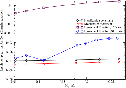
Figure 1: Accuracy for Einstein equations resolution (in the original (3+1) version of York79 ) as a function of dimensionless parameter $M_{\mathcal{H}}\Omega$ (see section V.3 for a definition of $M_{\mathcal{H}}$). Data are absolute maximum error values for both constraint equations, and dynamical equations in both cases. Data are taken with $N_{r}=33$, $N_{\theta}=17$, $N_{\varphi}=1$. Lapse on the horizon is $N_{\mathcal{H}}=0.55$.

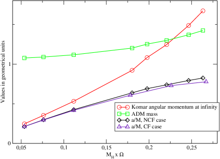
Figure 2: Dependence on the parameter $M_{\mathcal{H}}\Omega$ of the ADM mass, the Komar angular momentum at infinity $J_{K}$ and the angular momentum parameter $\frac{a}{M}$ (both defined in section IV.1) for both cases. The value of the lapse on the horizon is here fixed at $N_{\mathcal{H}}=0.55$.

Let us mention again the remark made by CookPf04 about the boundary condition for the lapse in the XCTS scheme. Although it is necessary to fix the slicing of the spacetime by an arbitrary boundary condition on the lapse, we have the freedom to decide what kind of condition to impose. The authors in CookPf04 suggest that an arbitrary condition of Neumann or Robin type would be preferable, because it is more flexible in view of a numerical algorithm. In particular, not fixing a value for the lapse on the horizon, but rather giving a first order prescription, allows the data to “adapt” to potentially high tidal distortions. However, having also tried to impose Neumann conditions for the lapse in our configurations, we do not see any clear improvement in the robustness of the algorithm. This is why we still keep a Dirichlet boundary condition as the simplest prescription.

V.3 Physical and geometrical tests for stationarity

One of the tests of stationarity to be made can be the comparison between the ADM mass and the Komar mass at infinity, defined with the (presumably) Killing vector $\left(\frac{\partial}{\partial t}\right)^{i}$ (equation (7.91) of Gourg07 ). The results of this test are displayed in figure 3. The comparison between the ADM mass and the Komar mass is actually directly linked to the Virial theorem of general relativity put forth by Virial94 . The concordance between those masses is equivalent to the vanishing of the Virial integral, and has been also used as a stationarity marker by GGB02 .

We have also computed in both NCF and CF cases an estimate of the amount of gravitational radiation contained outside the black hole in the 3-slice. Following the prescriptions of AshBF , we calculate the difference between the ADM mass and what could be called the isolated horizon mass, defined in geometrical units by:

$$M_{\mathcal{H}}=\frac{\sqrt{R_{\mathcal{H}}^{4}+4J_{\mathcal{H}}^{2}}}{2R_{\mathcal{H}}}.$$ (36)

where $R_{\mathcal{H}}$ is the areal radius of $\mathcal{H}$. $M_{\mathcal{H}}$ is nothing but the formula for the Christodoulou mass Christ calculated from the Komar angular momentum $J_{\mathcal{H}}$ on the horizon (defined with the same supposed Killing symmetry as $J_{K}$). If we have an isolated horizon extending to future infinity, the difference between $M_{ADM}$ and $M_{\mathcal{H}}$ gives exactly the radiation energy emitted at future null infinity for the data AshBF . In non-stationary cases (for example binary systems), this is an appropriate estimate of the radiation content at an initial given time.

Results for comparison between the two cases studied here are shown in figure 3. Although the gravitational energy available for NCF spacetimes is contained under $10^{-7}$ whatever the rotation rate might be, in the CF case, the increase in energy with $\frac{a}{M}$ is patent. This measure of energy available with respect to $\frac{a}{M}$ gives us a way of approximating a priori the amount of what is usually called “junk” gravitational radiation, that could be emitted on a spacetime evolution with conformally flat initial data.

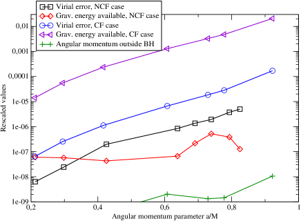
Figure 3: Different diagnostics for stationarity in both cases, comparing physical quantities at the horizon and at infinity. The virial error computes the difference between ADM and Komar masses at infinity, rescaled with the ADM mass, and using asymptotic behaviors of the lapse and conformal factor. The radiation energy content outside the black hole (resp. outer angular momentum content) is the absolute difference between the horizon mass $M_{\mathcal{H}}$ (resp. angular momentum on the horizon $J_{\mathcal{H}}$) and the ADM mass $M_{ADM}$ (resp. Komar angular momentum at infinity $J_{K}$), rescaled with the ADM mass (resp. Komar angular momentum at infinity).

In the same spirit, we have also computed the accuracy in the verification of a Penrose-like inequality for axisymmetric data, that can be written as:

$$\epsilon_{A}=\frac{\mathcal{A}}{8\pi(M_{ADM}^{2}+\sqrt{M_{ADM}^{4}-J_{K}^{2}})}\leq 1,$$ (37)

where $\mathcal{A}$ is the minimal area of a surface containing the horizon, $J_{K}$ is the Komar angular momentum at infinity and $M_{ADM}$ is the ADM mass at infinity. Being a little more stringent that the actual Penrose inequality, it has been first proposed by HawEll73 for axisymmetric spacetimes. This inequality is supposed to be verified for all axisymmetric data containing an apparent horizon, and to be an equality only for actual Kerr data (this is referred in JAV07 as Dain’s rigidity conjecture DaiLouTak02 ). The results are presented in figure 4. We observe that, if the equality is very well verified in the actual Kerr case, this is definitely not true for CF data, even for reasonable values of $\frac{a}{M}$. In JAV07 (cf. JarVal07 for a general context), it has been proposed that this quantity $\epsilon_{A}$ (Dain’s number) should be understood as a strong diagnosis tool for distinguishing between Kerr horizons and other isolated or dynamical horizons. This numerical observation shows strong support in favor of this claim, pulling apart actual Kerr data and reasonable approximations of these data. Let us also point out the virtual costlessness of this tool, as we only have to rely on a single real value.

We also note that, when computing the rescaled difference of Komar angular momentum between the horizon and infinity $\frac{J_{K}-J_{\mathcal{H}}}{J_{K}}$, we come up in all cases with a difference at the level of numerical precision for resolution (see figure 3). This is of course coherent with the fact that gravitational waves cannot carry any angular momentum in axisymmetric spacetimes. This result ensures us the equivalence in practice between the estimation of radiation exterior to the horizon and the verification of Penrose inequality via Dain’s number.

V.4 Multipolar analysis

To be much more complete about the geometry of the constructed horizons, one could rely on the source multipole decomposition of the two-surface lying on our three-slice. This feature has first been presented by AshENPVDB , based on an analogy with electromagnetism, and first studied in SchKriBey06 in the case of dynamical horizons. We here implement the computation of multipole moments in the isolated horizon case, which is the strict situation where they have been defined in AshENPVDB .

A prerequisite is the existence of a preferred divergence-free vector field $\varphi^{a}$ on the sphere, from which the angular momentum of the horizon is defined (the divergence-free condition on $\varphi^{a}$ ensures that all definitions will be gauge-independent). As mentioned above, our chosen vector field will be the one associated with the azimuthal coordinate, namely $\left(\frac{\partial}{\partial\varphi}\right)^{i}$.

Another important feature is the construction of a preferred coordinate system, so that the Legendre polynomials associated with spherical harmonics will possess the right orthonormality properties; as expressed in the implementation of SchKriBey06 , this reduces to finding a set of coordinates $(\zeta,\varphi)$ where the metric on the two-surface can be written as:

$$q^{\mathcal{H}}_{ab}=R_{\mathcal{H}}^{2}\left(f(\zeta)^{-1}D_{a}\zeta D_{b}\zeta+f(\zeta)D_{a}\varphi D_{b}\varphi\right),$$ (38)

with $R_{\mathcal{H}}$ the areal radius of the sphere and $f(\zeta)$ determined in terms of the two-dimensional Ricci scalar and the norm of $\varphi^{a}$ AshENPVDB . In the axisymmetric case studied here for the horizon, the integral curves for the coordinate $\varphi$ are already defined by the orbits of the vector field $(\frac{\partial}{\partial\varphi})^{i}$. The coordinate $\zeta$ is defined by

$$D_{a}\zeta=\frac{1}{R_{\mathcal{H}}^{2}}\epsilon_{ba}\varphi^{b}.$$ (39)

An appropriate normalization should be added, that ensures that $\oint_{\mathcal{H}}\zeta d^{2}V=0$. In the Kerr case, those coordinates turn out to correspond with the Boyer-Lindquist coordinates, with $\zeta=\cos{\theta}$ in spherical coordinates SchKriBey06 .

The mass and angular momentum multipoles of order $n$ are then defined, by analogy with electromagnetism AshENPVDB :

$$M_{n} = \frac{R_{\mathcal{H}}^{n}M_{\mathcal{H}}}{8\pi}\oint_{\mathcal{S}}\{\mathcal{R}P_{n}(\zeta)\}d^{2}V,$$ (40)

$$J_{n} = \frac{R_{\mathcal{H}}^{n-1}}{8\pi}\oint_{\mathcal{S}}P^{{}^{\prime}}_{n}(\zeta)K_{ab}s^{a}\varphi^{b}d^{2}V.$$ (41)

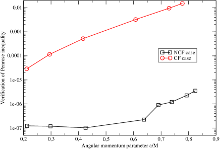
Figure 4: Value of $1-\epsilon_{A}$ for both data sets.

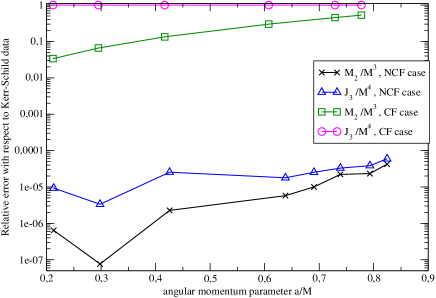
Figure 5: Computations of the rescaled second-order mass multipole $\left(\frac{M_{2}}{M^{3}}\right)$ and the rescaled third-order angular multipole $\left(\frac{J_{3}}{M^{4}}\right)$. Relative differences with respect to values for a Kerr-Schild analytical horizon are displayed.

With this definition and using the Gauss-Bonnet theorem it is trivial to see that $M_{0}=M_{\mathcal{H}}$ and $J_{1}=J_{K}$, the Komar angular momentum on the horizon.

We should emphasize that these multipoles, except for $M_{0}$ and $J_{1}$, are in general different from the field gravitational multipoles that can be defined at infinity. However, the authors in AshENPVDB have pointed out that the knowledge of all the multipoles of an isolated horizon allows to reconstruct the whole horizon, and also the spacetime in a vicinity of this horizon. The multipoles then discriminate exactly every isolated horizon, and the spacetime at its vicinity. Figure 5 shows the capacity of telling apart the horizon of a CF axisymmetric slice and the one of a NCF slice, in Dirac gauge. Data are also compared with an analytic Kerr solution in Kerr-Schild coordinates. Apart from the accuracy obtained for our NCF data (and a further confirmation that we indeed have obtained the actual Kerr spacetime), we see the clear distinction made by this computation between the Kerr horizon and a conformal approximation of it. Together with Dain’s number, this study has proven that those two tools are very well-suited to study isolated horizon properties, and the distance between data obtained from, say an evolution scheme, and the eventual equilibrium black hole data it is supposed to reach. Ultimate tests on the characterization of the obtained data as slices of Kerr could be achieved by implementing the schemes proposed in GarVal08 ; FerSae08 .

VI Discussion

The data we get with our simulations are interesting at several levels. They allow to make a direct comparison between the conformally flat approximation and the exact solution for axisymmetric spacetimes containing a black hole, that are both calculated a priori and in the same gauge. As we have seen in Sec. V, this gives us insight about the geometric features of the exact solution; we can single important issues concerning for example the intrinsic geometry of the horizon, via multipoles and the Penrose inequalities. Numerical tools are in this respect implemented and their efficiency tested.

At a more theoretical level, the method we used to get those data is a little bit heterodox: providing standard non-expanding horizon conditions for (3+1) variables such as $\beta^{i}$, $\psi$ and $N\psi$, we choose in addition not to prescribe any further geometrical information for the conformal part, symbolized here by the tensorial field $h^{ij}$. This has been motivated by the fact that, given the tensorial equation corresponding to $h^{ij}$ in our formalism, it appears that we most likely cannot prescribe anything else in the studied setting. By numerical transformation of the operator acting on $h^{ij}$ we ensured that at every iteration step no boundary condition was required. The fact that our system of Einstein equations written this way converges to the required Kerr solution shows that indeed, no additional information was needed in the single horizon case. To be more precise, our method suggests that in this case, the conformal geometry of the MOTS is directly encoded in the Einstein equations, when written with an equilibrium ansatz: we directly use these equations to justify a no-boundary treatment.

In the light of this numerical study, we can make a parallel with the proposition made in CookBaum08 . In that paper, the authors suggested, after a gauge dependence analysis for $\tilde{\gamma}^{ij}$ on the horizon, that a prescription could be made for the conformal geometry on the horizon. In this respect, they justify, for the projection of the three-metric on the two-surface, the following choice:

$$q_{ab}=\omega^{2}f_{ab},$$ (42)

with $f_{ab}$ the usual diagonal round metric for a two-sphere in spherical coordinates adapted to the horizon. This choice should not affect the physics of the three-slice, and suffices to recover the solution for Einstein dynamical equation with a slice of a spacetime containing an isolated horizon. Their study is made in a differential gauge generalizing the Dirac gauge we are using, namely $\mathcal{D}_{i}\tilde{\gamma}^{ij}=V^{i}$, with $V^{i}$ a regular vector field on the three-slice. Our case corresponds to $V^{i}=0$, which is precisely the one treated in detail in CookBaum08 .

When comparing to our data, we find that the projection of our three-metric on the two-surface is not conformally related to the flat metric in adapted spherical coordinates. This means that in our particular case, and in regard of the particular no-boundary argument we use, a boundary condition of the same type as (42) is probably inconsistent with our data, and is likely a choice that we do not have the freedom to make (note however that geometric conditions in Jaram08 making full use of the isolated horizon structure are indeed compatible with the present results, i.e. they are identically satisfied in the present Kerr case, whose horizon is indeed an isolated horizon). Unfortunately, the authors in CookBaum08 did not present any numerical results to support their claims, that we could have compared with ours.

We insist here on an important caveat for our argumentation: assumptions can only be justified in the very particular case we are studying here, which is the axisymmetric vacuum spacetime. This spacetime has very specific and non-trivial properties, all related to the uniqueness theorem of Carter Carter72 . Although the reasoning we have made on Sec. III for the operator could apply in other isolated horizon studies, we are not certain that our algorithm would globally converge when applied to a more general case (e.g. a black-hole binary system); a failure of this behavior would probably mean that an additional information about the conformal two-geometry has to be given to the system. Geometric fully isolated horizon boundary conditions proposed in Jaram08 could then be enforced (note that geometric inner boundary conditions in Jaram08 are not necessarily tied to the particular analytic setting here discussed and, more generally, they would also apply in schemes not enforcing the coordinate adaptation to stationarity at the horizon, $b=N_{\mathcal{H}}$, crucial for the singular nature of operators (30)).

Finally, let us point out the fact that we made those simulations by prescribing only the geometry of the horizon, and the geometry of spacetime at infinity. No assumption has been made for axisymmetry in the three-slice (computations can easily be made in the full 3D case and give the same results). Prescribing a vanishing expansion and a conformal Killing symmetry on a horizon, together with asymptotically flat hypothesis, our code converges to the only solution of the Kerr spacetime. Without claiming any rigorous demonstration here, this numerical result is most likely a support to the well known black hole rigidity theorem HawEll73 , where the same hypotheses lead to a uniqueness theorem involving the Kerr solution as the only one with no electromagnetic field.

VII Conclusion

We have used the prescription for a fully constrained scheme of (3+1) Einstein equations in generalized Dirac gauge Bon04 ; Cord1 to retrieve stationary axisymmetric black hole spacetime, and compared it with the analytical solution of Kerr type. An advanced handling of the conformal geometry of our three-slice allowed us to reach actual stationarity with good resolution precision for our scheme. Although we used standard quasi-equilibrium conditions concerning boundary values for other metric fields in the excised horizon, we found that the conformal geometry on the horizon required no prescription whatsoever in the single horizon case. This is in contrast with suggestions available in the literature CookBaum08 , and probably suggests an underlying physical feature of the horizon geometry (maybe related to uniqueness of the Kerr solution). To our knowledge, it is the first time the conformal part is numerically computed in a black hole spacetime using only a prescription on the stationarity of spacetime (and without resorting to additional symmetries). The application of this feature to the more general initial data problem is evident: in the same spirit as the work done in ShibLim for neutron-star binaries, using it for the black-hole binary system could lead to significant improvement in the available initial data for evolution codes. Further numerical work will clarify this issue.

We have implemented and used in our study numerical tools aimed at characterizing the geometry and physical properties related to horizons embedded in spacetime; those tools, among which a complete multipole analysis for two-surfaces as gravitational sources, have proven very accurate for diagnostics involving the horizon geometry and physical features. They will be more thoroughly presented, and tested in more general cases, in an upcoming work.

Appendix A Tensor spectral quantities adapted to the Dirac Gauge

We here give the definition of the three spectral quantities introduced in Sec. III.3, that describe the divergence-free degrees of freedom (with respect to the Dirac gauge) associated with a rank two symmetric tensor. The reader is also invited to go to Cord2 or NovCV where more detailed calculations are provided.

We first define a set of spin-weighted tensor spherical harmonics components for a symmetric rank-2 tensor, directly linked to the tensor spherical harmonics as introduced by Mathews and Zerilli MathZer1 ; MathZer2 . We shall give the expression for these components of the tensor $h^{ij}$ using the classical spherical coordinate basis, which is used in practice in our computations. With the notation $P=h^{\theta\theta}+h^{\varphi\varphi}$, the six pure spherical harmonics components of $h^{ij}$ are defined as :

$$\Delta_{\theta\varphi}\eta = \frac{\partial h^{r\theta}}{\partial\theta}+\frac{h^{r\theta}}{\tan\theta}+\frac{1}{\sin\theta}\frac{\partial h^{r\varphi}}{\partial\varphi},$$ (43)

$$\Delta_{\theta\varphi}\mu = \frac{\partial h^{r\varphi}}{\partial\theta}+\frac{h^{r\varphi}}{\tan\theta}-\frac{1}{\sin\theta}\frac{\partial h^{r\theta}}{\partial\varphi},$$ (44)

$$\Delta_{\theta\varphi}\left(\Delta_{\theta\varphi}+2\right)\mathcal{W} = \frac{\partial^{2}P}{\partial\theta^{2}}+\frac{3}{\tan\theta}\frac{\partial P}{\partial\theta}-\frac{1}{\sin^{2}\theta}\frac{\partial^{2}P}{\partial\varphi^{2}}$$

$$-2P + \frac{2}{\sin\theta}\frac{\partial}{\partial\varphi}\left(\frac{\partial h^{\theta\varphi}}{\partial\theta}+\frac{h^{\theta\varphi}}{\tan\theta}\right),$$ (45)

$$\Delta_{\theta\varphi}\left(\Delta_{\theta\varphi}+2\right)\mathcal{X} = \frac{\partial^{2}h^{\theta\varphi}}{\partial\theta^{2}}+\frac{3}{\tan\theta}\frac{\partial h^{\theta\varphi}}{\partial\theta}-\frac{1}{\sin^{2}\theta}\frac{\partial^{2}h^{\theta\varphi}}{\partial\varphi^{2}}$$

$$-2h^{\theta\varphi} - \frac{2}{\sin\theta}\frac{\partial}{\partial\varphi}\left(\frac{\partial P}{\partial\theta}+\frac{P}{\tan\theta}\right),$$ (46)

the fifth and sixth scalar fields being simply the tensor trace $h$ with respect to the flat metric and the $h^{rr}$ spherical component. Let us note that these relations are more tractable when using a scalar spherical harmonics decomposition (introduced in Sec. IV.2) for all fields. Indeed, an angular Laplace operator acting on a field reduces then to a simple algebraic operation on every spherical harmonics component. Inverse relations can also be computed to retrieve the classical components of $h^{ij}$ from spherical harmonics quantities.

We now derive the main variables related to our study: with the divergence-free decomposition $h^{ij}=\mathcal{D}^{i}W^{j}+\mathcal{D}^{j}W^{i}+h^{ij}_{T}$, and $\mathcal{D}_{i}h^{ij}_{T}=0$, a choice for three quantities defined from $h^{ij}$ and verifying:

$$h^{ij}_{T}=0\Rightarrow A=B=C=0,$$ (47)

can be expressed as the following scalar fields (see NovCV ):

$$A=\frac{\partial{\cal X}}{\partial r}-\frac{\mu}{r},$$ (48)

$$B=\frac{\partial{\cal W}}{\partial r}-\frac{\Delta_{\theta\varphi}{\cal W}}{2r}-\frac{\eta}{r}+\frac{h-h^{rr}}{4r},$$ (49)

$$C=\frac{\partial(h-h^{rr})}{\partial r}-\frac{3h^{rr}}{r}+\frac{h}{r}-2\Delta_{\theta\varphi}\left(\frac{\partial{\cal W}}{\partial r}+\frac{{\cal W}}{r}\right)$$ (50)

These quantities can also be decomposed onto a scalar spherical harmonics basis. The equivalence in (47) is achieved up to boundary conditions.

To show how the quantities $A$, $B$ and $C$ behave with respect to the Laplace operator, we shall assume in the following that the tensor $h^{ij}$ is the solution of a Poisson equation of the type $\Delta h^{ij}=S^{ij}$. We can deduce a scalar elliptic system verified by $A$, $B$ and $C$ as:

$$\Delta A=A_{S}$$ (51)

$$\Delta B-\frac{C}{2r^{2}}=B_{S}$$ (52)

$$\Delta C+\frac{2C}{r^{2}}+\frac{8\Delta_{\theta\varphi}B}{r^{2}}=C_{S},$$ (53)

Where $A_{S}$, $B_{S}$ and $C_{S}$ are the corresponding quantities associated with the source $S^{ij}$. A simple way of decoupling the last two elliptic equations is to define the variables $\tilde{B}=\sum_{l,m}\tilde{B}^{lm}Y_{lm}$ and $\tilde{C}=\sum_{l,m}\tilde{C}^{lm}Y_{lm}$ with:

$$\tilde{B}^{lm}=B^{lm}+\frac{C^{lm}}{2(l+1)},$$ (54)

$$\tilde{C}^{lm}=C^{lm}-4lB^{lm}.$$ (55)

Thus, we can write an equivalent system for (51,52,53) as:

$$\Delta A = A_{S},$$ (56)

$$\tilde{\Delta}\tilde{B} = \tilde{B}_{S},$$ (57)

$$\Delta^{*}\tilde{C} = \tilde{C}_{S},$$ (58)

With the following elliptic operators defined for each spherical harmonic index l:

$$\Delta = \frac{\partial^{2}}{\partial r^{2}}+\frac{2}{r}\frac{\partial}{\partial r}-\frac{l(l+1)}{r^{2}}I$$ (59)

$$\tilde{\Delta} = \Delta+\frac{2l}{r^{2}}I,$$ (60)

$$\Delta^{*} = \Delta-\frac{2(l+1)}{r^{2}}I.$$ (61)

$I$ is the identity operator. $A$, $\tilde{B}$ and $\tilde{C}$ are then defined as three scalar fields characterizing only the divergence-free part of a symmetric rank two tensor $h^{ij}$, and giving a system of three decoupled scalar elliptic equations in the Poisson problem for this tensor. Hence they are very well suited to the study of a tensorial elliptic problem in Dirac gauge. Let us finally note that the quantities $\tilde{B}$ and $\tilde{C}$ are directly related to each other by the trace of the considered tensor NovCV : If we know a priori the value of the trace for $h^{ij}$, then the knowledge of $\tilde{B}$ suffices to recover $\tilde{C}$ with no additional information (the converse being equally true).

Appendix B Recovery of $h^{ij}$ from $A$ and $\tilde{B}$

In this section, we come up with technical details for resolution of the gauge differential system introduced in Sec. III.3, to reconstruct the tensor $h^{ij}$ from the quantities $A$ and $\tilde{B}$.

We begin by expressing components of the vector field representing the divergence of $h^{ij}$:

$$H^{i}=\mathcal{D}_{i}h^{ij},$$ (62)

with the Dirac gauge for $H^{i}=0$. Adopting the vector spherical harmonics decomposition suggested in Bon04 , the three spherical harmonics components of $H^{i}$ are expressed, in function of the spherical harmonics components of $h^{ij}$ (see Appendix A), as:

$$H^{r} = \frac{\partial h^{rr}}{\partial r}+\frac{3h^{rr}}{r}+\frac{1}{r}\left(\Delta_{\theta\varphi}\eta-h\right),$$ (63)

$$H^{\eta}\! = \!\Delta_{\theta\varphi}\left[\frac{\partial\eta}{\partial r}+\frac{3\eta}{r}+\frac{1}{r}\left(\left(\Delta_{\theta\varphi}+2\right)\mathcal{W}+\frac{h-h^{rr}}{2}\right)\right],$$ (64)

$$H^{\mu} = \Delta_{\theta\varphi}\left[\frac{\partial\mu}{\partial r}+\frac{3\mu}{r}+\frac{1}{r}\left(\Delta_{\theta\varphi}+2\right)\mathcal{X}\right].$$ (65)

Those three expressions, alongside with definitions of the quantities $A$ and $\tilde{B}$, will allow to express two decoupled differential systems. The first one, involving the spherical harmonics components $\mu$ and $\mathcal{X}$, combines the expression for the scalar field $A$, as well as the fact that $H^{\mu}$ vanishes under the Dirac gauge :

$$\left\{\begin{aligned} &\frac{\partial{\cal X}}{\partial r}-\frac{\mu}{r}=A,\\ &\frac{\partial\mu}{\partial r}+\frac{3\mu}{r}+\frac{1}{r}\left(\Delta_{\theta\varphi}+2\right)\mathcal{X}=0.\end{aligned}\right.$$ (66)

The second system is composed of the definition of $\tilde{B}$ for each of its spherical harmonic component $\tilde{B}^{lm}$, as well as the vanishing of $H^{r}$ and $H^{\eta}$(again, due to Dirac gauge):

$$\left\{\begin{aligned} &\tilde{B}^{lm}=B^{lm}+\frac{C^{lm}}{2(l+1)},\\ &\frac{\partial h^{rr}}{\partial r}+\frac{3h^{rr}}{r}+\frac{1}{r}\left(\Delta_{\theta\varphi}\eta-h\right)=0,\\ &\frac{\partial\eta}{\partial r}+\frac{3\eta}{r}+\frac{1}{r}\left(\left(\Delta_{\theta\varphi}+2\right)\mathcal{W}+\frac{h-h^{rr}}{2}\right)=0.\end{aligned}\right.$$ (67)

with the expressions (49, 50) of $B$ and $C$ as functions of the spherical harmonics components of $h^{ij}$. In this system, the trace is given a priori, so that only three spherical harmonics components are considered as unknowns.

We refer to the analysis of NovCV to affirm that, when solving our equations in $\mathbb{R}^{3}$ minus an excised inner sphere, one boundary condition has to be provided at the surface for the system (66), and two for the system (67). As pointed out in Sec.IV.2, these conditions are retrieved as compatibility conditions based on the original elliptic tensorial equation. Overall, we are able to invert the two Dirac differential systems, and retrieve all the spherical harmonics components of $h^{ij}$ from the sole knowledge of $A$, $\tilde{B}$ and the trace $h$.

References

- (1) F. Pretorius, Phys. Rev. Lett. 95, 121101 (2005).
- (2) M. Campanelli, C. O. Lousto, P. Marronetti and Y. Zlochower, Phys. Rev. Lett. 96, 111101 (2006).
- (3) J. G. Baker, J. Centrella, D. Choi, M. Koppitz and J. Van Meter, Phys. Rev. Lett. 96, 111102 (2006).
- (4) F. Pretorius, to appear in Relativistic Objects in Compact Binaries: From Birth to Coalescence (2008), arXiv:0710.1338
- (5) S. Brandt and B. Bruegmann, Phys. Rev. Lett. 78, 3606–3609 (1997).
- (6) F. Foucart, L. Kidder, H. Pfeiffer and S. Teukolsky, Phys. Rev. D 77, 124051 (2008).
- (7) B. Szilagyi, D. Pollney, L. Rezzolla, J. Thornburg and J. Winicour, Class. Quant. Grav. 24 S275 (2007). [arXiv:gr-qc/0612150].
- (8) U. Sperhake, Phys. Rev. D 76, 104015 (2007).
- (9) S. Hawking and J. B. Hartle, Comm. Math. Phys. 27, 283–290 (1972).
- (10) T. Damour, Thèse de Doctorat d’État, Université Paris VI (1979).
- (11) K. Thorne, R. Price and D. MacDonald, Black Holes: The membrane paradigm, Yale University Press (1986).
- (12) I. Booth, Can. J. Phys. 83, 1073 (2005).
- (13) S. Hayward, Phys. Rev. D 49, 6467 (1994).
- (14) A. Ashtekar, C. Beetle and S. Fairhurst, Class. Quantum Grav. 16, L1–L7 (1999).
- (15) A. Ashtekar and B. Krishnan, Phys. Rev. D 68, 104030 (2003).
- (16) R. Penrose, Phys. Rev. Lett. 14, 57 (1965).
- (17) E. Gourgoulhon, Phys. Rev. D 72, 104007 (2005).
- (18) E. Gourgoulhon and J. L. Jaramillo, Phys. Rev. D 74, 087502 (2006).
- (19) G. B. Cook, Phys. Rev. D 65, 084003 (2002).
- (20) J. L. Jaramillo, E. Gourgoulhon and J. M. Mena Marugàn, Phys. Rev. D 70, 124036 (2004).
- (21) E. Gourgoulhon and J. L. Jaramillo, Phys. Rep. 423, 159 (2006).
- (22) G. B. Cook and H. Pfeiffer, Phys. Rev. D 70, 104016 (2004).
- (23) M. Caudill, G. B. Cook, J. D. Grigsby, & H. P. Pfeiffer, Phys. Rev. D 74, 064011 (2006).
- (24) J. L. Jaramillo, M. Ansorg and F. Limousin, Phys. Rev. D 75, 024019 (2007).
- (25) S. Bonazzola, E. Gourgoulhon, P. Grandclément and J. Novak, Phys. Rev. D 70, 104007 (2004).
- (26) I. Cordero-Carrión, P. Cerdá-Durán, H. Dimmelmeier, J. L. Jaramillo, J. Novak and E. Gourgoulhon, E., Phys. Rev. D.79, 024017 (2009).
- (27) http://www.lorene.obspm.fr
- (28) S. Hawking and G. Ellis, The large Scale Structure of Spacetime, Cambridge University Press (1973).
- (29) J. M. M. Senovilla, AIP Conf. Proc. 1122, 72 (2009).
- (30) A. Ashtekar and B. Krishnan, Living Rev. Relativity 7, 10 (2004), http://www.livingreviews.org/lrr-2004-10.
- (31) P. Hajiček, Comm. Math. Phys. 34, 37 (1973).
- (32) J. Thornburg, Living Rev. Relativity 10, 3 (2007), http://www.livingreviews.org/lrr-2007-3.
- (33) L. M. Lin and J. Novak, Class. Quantum Grav. 24, 2665 (2007).
- (34) C. Gundlach, Phys. Rev. D 57, 863–875 (1998).
- (35) J. Thornburg, Class. Quantum Grav. 21, 743–766 (2004).
- (36) O. Dreyer, B. Krishnan, E. Schnetter and D. Shoemaker, Phys. Rev. D 67, 024018 (2003).
- (37) E. Schnetter, B. Krishnan, & F. Beyer, Phys. Rev. D74, 024028 (2006).
- (38) S. Dain, J.L. Jaramillo, and B. Krishnan, Phys. Rev. D 71, 064003 (2005).
- (39) G. B. Cook and T. Baumgarte, Phys. Rev. D 77, 064023 (2008).
- (40) J. W. York, in Sources of Gravitational Radiation, Cambridge University Press (1979).
- (41) E. Gourgoulhon, Formalism and bases of numerical relativity, lectures at Institut Henri Poincaré, Paris (2006), arXiv:gr-qc/0703035
- (42) M. Alcubierre, Introduction to numerical relativity (Oxford University Press, Oxford, 2008).
- (43) R. Arnowitt, S. Deser and C. W. Misner, The dynamics of General Relativity, in Gravitation: an introduction to current research, Wiley, New York, 227–265 (1962).
- (44) A. Lichnerowicz, J. Math. Pures. Appl. 23, 37 (1944).
- (45) A. Garat and R. H. Price, Phys. Rev. D 61, 124011 (2000).
- (46) J. A. Valiente Kroon, Phys. Rev. Lett. 92, 041101 (2004).
- (47) P. Cerdá-Durán, G. Faye, H. Dimmelmeier, J. A. Font, J. M. Ibáñez, E. Müller, and G. Schäfer, Astron. Astrophys. 439, 1033 (2005).
- (48) S. Brandt and E. Seidel, Phys. Rev. D 54, 1403 (1996).
- (49) K. Uryu, F. Limousin, J. Friedman, E. Gourgoulhon and M. Shibata, Phys. Rev. Lett. 97, 171101 (2006).
- (50) M. Shibata, K. Uryu and J. Friedman J., Phys. Rev. D 70, 044044 (2004).
- (51) L. M. Lin and J. Novak, Class. Quantum Grav. 23, 4545 (2006).
- (52) I. Cordero-Carrión, J. M. Ibánez, E. Gourgoulhon, J. L. Jaramillo and J. Novak, Phys. Rev. D 77, 084007 (2008).
- (53) J. Novak, J. L. Cornou and N. Vasset,[arXiv:gr-qc/0905.2048].
- (54) J. L. Jaramillo, E. Gourgoulhon, I. Cordero-Carrión and J. M. Ibánez, Phys. Rev. D 77, 047501 (2008).
- (55) E. Hairer, S. D. Norsett and G. Wanner, Ordinary Differential Equations I, Springer-Verlag (1987).
- (56) P. Grandclément and J. Novak, Living Rev. Relativity 12, 1 (2009), http://www.livingreviews.org/lrr-2009-1.
- (57) J. A. Isenberg, Int. J. Mod. Phys. D 17, 265 (2008).
- (58) J. Wilson and G. Mathews, Relativistic hydrodynamics, Frontiers in Numerical Relativity, Cambridge university press (1989).
- (59) E. Gourgoulhon and S. Bonazzola, Class. Quantum Grav. 11, 443–452 (1994).
- (60) E. Gourgoulhon, P. Grandclément and S. Bonazzola, Phys. Rev. D 65, 044020 (2002).
- (61) D. Christodoulou, PhD thesis, Princeton university, unpublished.
- (62) S. Dain, C. O. Lousto, and R. Takahashi, Phys. Rev. D 65(10), 104038 (2002).
- (63) J. L. Jaramillo, M. Ansorg and N. Vasset, in proceedings of the Spanish Relativity meeting, arXiv:0712.1741.
- (64) J. L. Jaramillo, J. A. Valiente Kroon and E. Gourgoulhon, Class. Quant. Grav. 25, 093001 (2008)
- (65) A. Ashtekar, J. Engle, T. Pawlowski and C. Van Den Broecke, Class. Quantum Grav. 21, 2549–2570 (2004).
- (66) A. Garcia-Parrado Gomez-Lobo and J. A. Valiente Kroon, Class. Quant. Grav. 25, 205018 (2008) arXiv:0805.4505.
- (67) J. J. Ferrando and J. A. Saez, Class. Quant. Grav. 26, 075013 (2009).
- (68) J. L. Jaramillo,Phys. Rev. D 79, 087506 (2009).
- (69) B. Carter, Phys. Rev. Lett. 26, 331–333 (1971).
- (70) J. Mathews, J. Soc. Ind. Appl. Math. 10, 768 (1962).
- (71) F. J. Zerilli, J. Math. Phys. 11, 2203 (1970).