Evidence of a link between the evolution of clusters and their AGN fraction

Abstract

We discuss the optical properties, X-ray detections, and Active Galactic Nucleus (AGN) populations of four clusters at $z\sim 1$ in the Subaru-XMM Deep Field (SXDF). The velocity distribution and plausible extended X-ray detections are examined, as well as the number of X-ray point sources and radio sources associated with the clusters. We find that the two clusters that appear virialised and have an extended X-ray detection contain few, if any, AGN, whereas the two pre-virialised clusters have a large AGN population. This constitutes evidence that the AGN fraction in clusters is linked to the clusters’ evolutionary stage. The number of X-ray AGN in the pre-virialised clusters is consistent with an overdensity of factor $\sim 200$; the radio AGN appear to be clustered with a factor of three to six higher. The median $K$-band luminosities of $L_{K}=1.7~{}\pm~{}0.7~{}L^{*}$ for the X-ray sources and $L_{K}=2.3~{}\pm~{}0.1~{}L^{*}$ for the radio sources support the theory that these AGN are triggered by galaxy interaction and merging events in sub-groups with low internal velocity distributions, which make up the cluster environment in a pre-virialisation evolutionary stage.

1 Introduction

A long-standing question in current astronomy is the connection between the formation of large-scale structure and galaxy formation and evolution. Studying clusters up to high redshifts gives us the ideal opportunity to study the interaction between galaxies and the intergalactic medium in detail, as a cluster’s deep potential well causes the cluster gas to be retained in the same environment. Frequently studied phenomena impacting galaxy evolution in clusters involve feedback mechanisms which couple the large-scale gaseous environment to the small-scale generation of jets from AGN. Jets and other AGN-driven outflows can heat and re-distribute the gas, perhaps suppressing star-formation in the cluster (e.g. Scannapieco & Oh 2004; Fabian,Celotti & Erlund 2006). As emphasised by Rawlings & Jarvis (2004), powerful radio jets can also have profound influence on the evolution of galaxies in protoclusters.

The correlation of radio-loud AGN and galaxy clusters has been studied over a range of redshifts. At low redshift, luminous radio galaxies tend to occur mostly in galaxy groups and low-mass clusters (e.g. Prestage & Peacock 1988, Hill & Lilly 1991, Miller et al. 2003). At higher redshifts ($z\sim 0.5$) however, it has been shown that approximately 40% of radio galaxies are located in massive clusters of Abell richness 0 and higher (e.g. Hill & Lilly 1991). Reaching a redshift of unity, some powerful radio sources are found at the centres of galaxy clusters (e.g. Best 2000). Searches for emission-line galaxies around radio galaxies at redshifts $z>2$ have shown that the latter often occur in (proto-) clusters (e.g. Venemans et al. 2002)

The launch of the Chandra X-ray Observatory in 1999 made it feasible to efficiently identify the prevalence of X-ray luminous AGN in clusters. Optical follow-up of X-ray point sources in the fields of rich clusters of galaxies have shown that clusters may contain a large fraction of optically obscured AGNs (e.g. Martini et al. 2002, 2006). Martini, Mulchaey & Kelson (2007) find that the fraction of X-ray selected AGN is similar in clusters and the field, contrary to optically selected AGN, although the fraction varies significantly between clusters.

The distribution of AGN in clusters provides meaningful information on the mechanism that triggers and sustains them. One such possible process is the interaction and merging of galaxies (e.g. Barnes & Hernquist 1996), enabling the creation of a central supermassive black hole and the matter to fuel it. In this case the AGN fraction would be determined by the properties of the environment providing the opportunities for interaction and the supply of fuel. These external conditions are likely to change in clusters as they evolve from merging sub-groups to a massive virialised cluster. Studying clusters at high redshifts and early evolutionary stages can therefore play a key role in understanding the correlation between the AGN fraction and their cluster environment.

In this paper we explore the AGN population of the highest-redshift clusters found by Van Breukelen et al. (2006, henceforth VB06) in the SXDF, using both radio and X-ray data to identify the AGN, and multi-object spectroscopy on both the clusters and active galaxies to determine their exact redshifts. This paper is organised as follows: in Section 2 we describe the spectroscopic observations and data reduction; Section 3 presents the properties of each of the clusters in our highest-redshift sample and in Section 4 we study the AGN population of our clusters. Section 5 contains a discussion of our conclusions. Throughout this paper we use the cosmological parameters $H_{0}=71~{}\rm km~{}s^{-1}$, $\Omega_{M}=0.3$ and $\Omega_{\Lambda}=0.7$.

2 The Data

2.1 The cluster sample

Figure 1: The positions of the three 5^′-radius cluster fields. CVB6 is centred on RA = $02^{\rm h}18^{\rm m}32.7^{\rm s}$, Dec = $-05^{\circ}01^{\prime}04^{\prime\prime}$; CVB11 is centred on RA = $02^{\rm h}18^{\rm m}06.4^{\rm s}$, Dec = $-05^{\circ}03^{\prime}25^{\prime\prime}$; and CVB13 is centred on RA = $02^{\rm h}18^{\rm m}09.0^{\rm s}$, Dec = $-05^{\circ}00^{\prime}29^{\prime\prime}$. Three-colour images of each of the fields can be found in Figs.8, LABEL:overlay11, and 10.

In this paper, we focus on the 5^′-radius cluster fields of CVB6 ($z=0.9$), CVB11 ($z=1.1$), and CVB13 ($z=1.3$). These are the highest-redshift clusters of VB06 with a significant number of spectroscopically confirmed cluster members ($\mathrel{\hbox{\hbox to0.0pt{\hbox{\lower 2.0pt\hbox{$\sim$}}\hss}\raise 2.0pt\hbox{$>$}}}10$). The positions of the three fields are depicted in Fig. 1.

The field of CVB13 has been studied extensively using DEIMOS spectroscopy by Van Breukelen et al. (2007, henceforth VB07). They show the field contains two clusters: CVB13A at $z=1.28$ and CVB13B at $z=1.45$. In this paper we focus solely on CVB13A as we now have a larger number of confirmed cluster members available for this cluster (see Section 3.3).

As will be discussed in Section 3.2, the cluster field of CVB11 also contains two clusters: CVB11A at $z=1.06$ and CVB11B at $z=1.09$. For the purposes of this paper, both clusters are included in our final sample which consequently comprises four clusters in three fields. Note that when we use the denominations ‘CVB11’ or ‘CVB13’ we are referring to the cluster fields, whereas the postfix ‘A’ or ‘B’ signifies the individual clusters.

2.2 Imaging Data

We use multi-wavelength data stemming from several surveys and datasets. The optical imaging data (mainly used to create three-colour images) are from the Subaru Telescope and comprise the $BVRi^{\prime}z^{\prime}$ bands (Furusawa et al. 2008). Near-infrared $J$ and $K$ data were taken from the Ultra Deep Survey on the United Kingdom InfraRed Telescope (UKIRT) (Foucaud et al. 2007). Further, we use X-ray data from the XMM-Newton satellite (Watson et al. 2004) and radio data (Simpson et al. 2006; Ivison et al. 2007) from the A- and B-array configurations of the Very Large Array (VLA).

Figure 2: Spectroscopic redshift histogram for the three cluster fields at $0.5\leq z_{\rm spec}\leq 1.5$. The shaded bins denote the galaxies observed with GMOS; the unfilled bins represent the DEIMOS targets. Note that the histograms for fields CVB11 and CVB13 are very similar as they largely overlap.

2.3 Spectroscopic Data

The spectroscopic data used in this paper originate from various sources. Firstly, a subset of the cluster galaxies was observed with the Deep Imaging Multi-Object Spectrograph (DEIMOS) on the Keck 2 telescope in Hawaii. The target selection, observations, and data reduction can be found in VB07. Secondly, we make use of the SXDF spectroscopic master list (maintained by C. Simpson and M. Akiyama, private communication). This list contains redshifts for sources in the SXDF/UDS derived from a number of observing runs on several telescopes. The data we use in this paper result from VIsible Multi-Object Spectrograph (Simpson et al. in preparation) and Faint Object Camera and Spectrograph (FOCAS) (Yamada 2005 and Akiyama et al. in preparation). Finally, the remainder of the cluster galaxies were observed on the Gemini North telescope in Hawaii with the Gemini Multi-Object Spectrograph (GMOS, Hook et al. 2004). These data are described below.

2.3.1 GMOS target selection

The targets for the spectroscopic data taken with GMOS were five candidate clusters, identified in VB06. We selected them from the clusters at photometric redshifts $0.8\mathrel{\hbox{\hbox to0.0pt{\hbox{\lower 2.0pt\hbox{$\sim$}}\hss}\raise 2.0pt\hbox{$<$}}}z_{\rm phot}\mathrel{\hbox{\hbox to0.0pt{\hbox{\lower 2.0pt\hbox{$\sim$}}\hss}\raise 2.0pt\hbox{$<$}}}1.0$. Since our telescope time was limited, we only targeted the clusters that had a possible associated X-ray detection. The resulting candidate clusters are given in the Appendix in Table 4.

For each cluster candidate, the target cluster galaxies for the MOS mask were selected based on the cluster-selection algorithm outlined in VB06. The algorithm presented in this paper used two methods to detect clusters: Voronoi Tesselations and Friends-of-Friends. To optimise the mask design, we divided the target galaxies into three priorities for each cluster:

1. all galaxies that were assigned to the cluster by both methods of the algorithm of VB06.

2. the galaxies that were assigned to the cluster by either of the methods of the algorithm of VB06.

3. all galaxies in the field-of-view of the GMOS instrument ($5.5^{\prime}\times 5.5^{\prime}$) with a photometric redshift within a 2-sigma range of the photometric redshift of the cluster candidate (see Table 4 in the Appendix).

The number of target galaxies for each cluster and the number of galaxies included in the MOS masks are given in Table 4 in the Appendix.

2.3.2 Spectroscopy on Gemini

The data from GMOS were taken between 2006 August 17 and December 25 in queue mode (program ID: GN-2006B-Q-44). The MOS mask contained slitlets of 1^′′ wide and 3^′′ long. To optimise the sky subtraction during data reduction, we used the Nod & Shuffle (N&S) mode with micro-shuffling. Each of our science exposures was divided into 28 N&S cycles of 60 seconds each, with 1.5^′′ nodding offsets on the sky and 3^′′ shuffling offsets on the CCD. We used the R400 grating with no filter and a central wavelength of 795 nm. The spectral resolution of this set-up was $\lambda/\Delta\lambda\approx 1700$. Each target cluster was observed in four integrations of 3360 seconds. To reduce the effect of charge traps, cosmic rays, bad pixels, and the gap between the two GMOS CCDs, each integration was offset by 5 nm in central wavelength (x-direction on the CCD) and a DTA-X offset was introduced of 0, 2, and 4 pixels (y-direction on the CCD). The binning on the CCD was $2\times 2$ pixels in the spatial and spectral directions, with an unbinned pixel size of 0.07^′′ per pixel. We maximised the number of cluster galaxies that could be observed in each MOS mask by choosing the optimal position angle of the instrument, which is given for each target cluster in Table 4 in the Appendix. The seeing was $\mathrel{\hbox{\hbox to0.0pt{\hbox{\lower 2.0pt\hbox{$\sim$}}\hss}\raise 2.0pt\hbox{$<$}}}0.80^{\prime\prime}$ for all targets and conditions were photometric throughout.

For calibration purposes, spectroscopic flatfields were taken after each exposure with a quartz-halogen lamp. We also executed a series of 35 darks to enable the removal of charge-traps during data reduction. Per target cluster, one arc exposure with a quartz-halogen lamp was taken for each central wavelength set-up. Finally, to allow flux calibration, we included observations of the spectrophotometric standard star BD+28d4211, using a longslit of 1^′′ width.

2.3.3 GMOS data reduction

The first step in the data reduction was the bias subtraction of the science and calibration frames, using bias exposures of the corresponding observing dates and set-ups taken from the Gemini archive. The science frames were sky subtracted and mosaicked using the Gemini data reduction tasks for IRAF. Next we combined the darks using the median value and identified the charge traps. These were subsequently masked out in the science frames. Finally the four science frames per target cluster were combined using the average value and a three-sigma clipping routine to remove cosmic rays and bad pixels.

We performed the flat-fielding, rectifying, cleaning and wavelength calibrations using a set of Python routines (Kelson, private communication). The final two-dimensional science frames were obtained by shifting the reduced image by the N&S offset and subtracting it from the original reduced image. The sensitivity function was derived in IRAF from the reduced spectrum of the standard star; this allowed the flux calibration of the two-dimensional science frames. We extracted the one-dimensional spectra using a boxcar extraction routine with an aperture of 1^′′.

2.4 Redshift determination

To determine the approximate redshifts of the galaxies observed both with GMOS and DEIMOS, we identified strong spectral features such as the [O ii]₃₇₂₇, H_β, and [O iii]_4960,5008 emission lines, the 4000-Å break, the Ca H&K absorption lines at 3933.4 and 3969.2 Å and the $G$ band at 4304.4 Å. For all galaxies showing the [O ii] emission line we determined the exact redshift by fitting a double Gaussian profile to the observed line profile, where the Full Width Half Maximum (FWHM) of each Gaussian was assumed to be equal, and was a free parameter of the fitted function. The other parameters were the redshift, the continuum level, and the ratio of fluxes of the two lines (see also VB07). The exact redshifts of the galaxies that only show absorption features were measured by cross-correlating their spectra with template spectral energy distributions. For this purpose we used a set of three stellar population synthesis templates from Bruzual & Charlot (2003), consisting of solar metallicity, 1-Gyr burst models of ages 3, 5, and 7 Gyr.

The spectroscopic redshifts obtained from the DEIMOS and GMOS data on each of the cluster fields of our sample are shown in Fig. 2. In the Appendix we show the result of a comparison between all spectroscopic redshifts and the photometric redshifts determined in VB06.

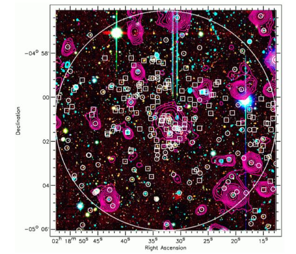
Figure 3: $Bi^{\prime}K$ image of cluster field CVB6. The large circle encompasses the $5^{\prime}$-radius field we investigate in this paper. The spectroscopic targets are marked by the white symbols: squares denote objects observed with GMOS and DEIMOS and circles are from the SXDF master list. Broadband XMM-Newton X-ray contours from a signal-to-noise map are overlaid in purple and VLA A-array (with a beam size of 1.9^′′ by 1.6^′′ at PA = 22^∘) contours in blue. The X-ray contours are at [$\sqrt{2}\sigma,2\sigma,2\sqrt{2}\sigma,...$], and the radio contours at [$2\sqrt{2}\sigma,4\sigma,4\sqrt{2}\sigma,...$].

3 Cluster properties

3.1 CVB6

3.1.1 Optical properties

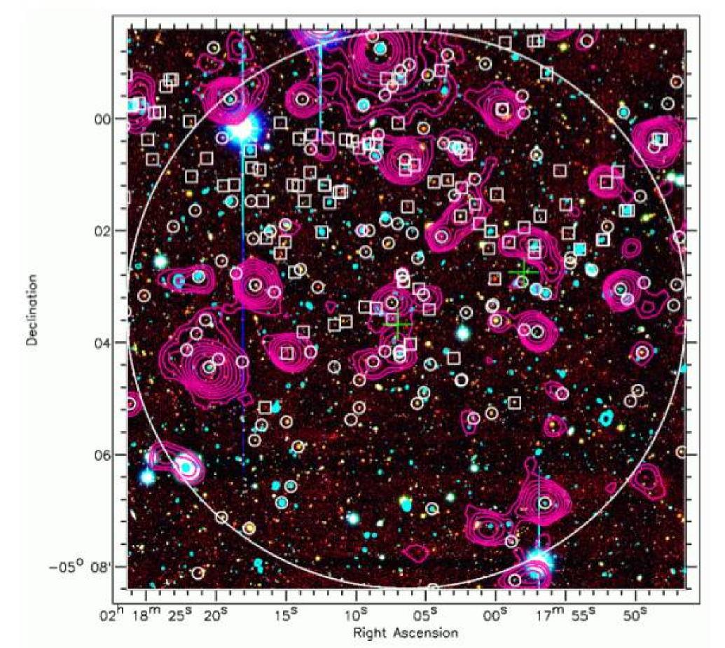
Figure 8: $Bi^{\prime}K$ image of cluster field CVB11. The green crosses denote the approximate positions of clusters CVB11A and CVB11B, based on the averages of the positions of the respective cluster galaxies. CVB11A is in the centre and CVB11B to the northwest. The other symbols and contours are as in Fig. 8.

The combined DEIMOS and GMOS spectroscopic data yielded 20 confirmed cluster galaxies for CVB6. This is the largest spectroscopic dataset we have available on any of our clusters. Fig. 8 shows all the data sets we use on the cluster field of CVB6: it is a $Bi^{\prime}K$ image with spectroscopic targets marked and X-ray and radio contours overlaid.

Figure 4: Velocity distribution of cluster CVB6. The overplotted Gaussian function is determined by $\overline{z}=0.87180\,\pm\,0.00007$ and $\sigma_{v}=608\,\pm\,115\,\rm km\,s^{-1}$. The shaded bins are objects from the SXDF master list.

Table 6 in the Appendix lists all cluster galaxies observed with GMOS and DEIMOS with their properties. We calculate the cluster redshift by taking the bi-weighted mean of the cluster galaxies (including the objects from the SXDF master list) as outlined by Beers et al. (1990). The velocity dispersion of the cluster is determined by selecting all galaxies within $\pm\,2000\,\rm km\,s^{-1}$ of the cluster redshift, and calculating the bi-weighted estimate of the scale factor of the distribution, which is assumed to be Gaussian. Fig. 4 shows the velocity distribution of the cluster, and the associated Gaussian function determined by $\overline{z}=0.87180\,\pm\,0.00007$ and $\sigma_{v}=608\,\pm\,115\,\rm km\,s^{-1}$. To calculate the virial mass of CVB6 we use the following empirical relation found by Evrard et al. (2008) through N-body simulations:

$$M_{200}=\frac{10^{15}h^{-1}{\rm M_{\odot}}}{H/H_{0}}\Big{(}\frac{\sigma_{\rm v,los}}{1083\,{\rm km\,s^{-1}}}\Big{)}^{3},$$ (1)

where $M_{200}$ is the mass contained within a sphere of radius $r_{200}$ for which the mean density is $200$ times the critical density $\rho_{\rm cr}$. We arrive at $M_{200}=1.6\times 10^{14}\,\rm M_{\odot}$ for CVB6.

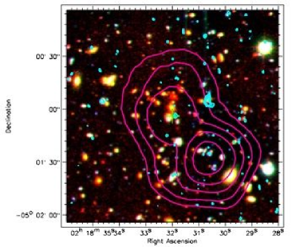
Figure 5: $Bi^{\prime}K$ image of the central $2^{\prime}$ of cluster CVB6 with broadband X-ray contours (from a signal-to-noise map) and 1.4 GHz radio contours overlaid in purple and blue respectively. The green cross denotes the position of the extended X-ray source. The X-ray point source to the southwest is a background object at $z=3.0$. The optical data is from the Subaru Telescope, the infrared data from UKIRT, the X-ray data from XMM-Newton, and the radio data from the VLA (A-array with a beam size of 1.9^′′ by 1.6^′′ at PA = 22^∘). The X-ray contours are at [$\sqrt{2}\sigma,2\sigma,2\sqrt{2}\sigma,...$], and the radio contours at [$2\sqrt{2}\sigma,4\sigma,4\sqrt{2}\sigma,...$].

3.1.2 X-ray emission from the intracluster medium

The 2XMM source catalogue (Watson et al. 2008) contains an X-ray source coincident with the position of cluster CVB6 which is extended over 20.4^′′ (the XMM point spread function is 6^′′). Fig. 5 shows a three colour image of the central $2^{\prime}$ of CVB6 with X-ray and radio contours overlaid. The extended emission is evident in the centre; to the southwest there is a background X-ray point source of total flux $4.1\,\pm\,0.6\times 10^{-17}\rm\,W\,m^{-2}$, associated with a spectroscopically confirmed quasar at $z=3.0$.

The total X-ray flux of the extended source is $3.91\,\pm\,1.05\times 10^{-17}\rm\,W\,m^{-2}$; its hardness ratios (HR) are $HR1=0.29\,\pm\,0.09$, $HR2=-0.02\,\pm\,0.08$, $HR3=-0.57\,\pm\,0.12$, and $HR4=0.26\,\pm\,0.24$. Here the hardness ratios are defined as $HR_{i}=(C_{i+1}-C_{i})/(C_{i}+C_{i+1})$, where $C_{i}$ is the count rate in band $i$. The energy bands are 1: 0.2 - 0.5 keV, 2: 0.5 - 1.0 keV, 3: 1.0 - 2.0 keV, 4: 2.0 - 4.5 keV, and 5: 4.5 - 12.0 keV. The source is sufficiently bright to construct an X-ray spectrum, which is shown in Fig. 6. The X-ray luminosity at $z=0.87$ is calculated to be $L_{\rm X}=1.45\times 10^{37}\rm\,W$.

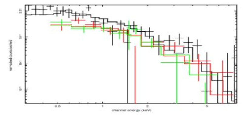
Figure 6: X-ray spectrum of cluster CVB6. The green and red symbols are the data from the two individual X-ray cameras (green: PN, red: M). The black data points is the combined result. The black line is a fit to the data using a black body ‘mekal’ emission spectrum and the ‘wabs’ local absorption model.

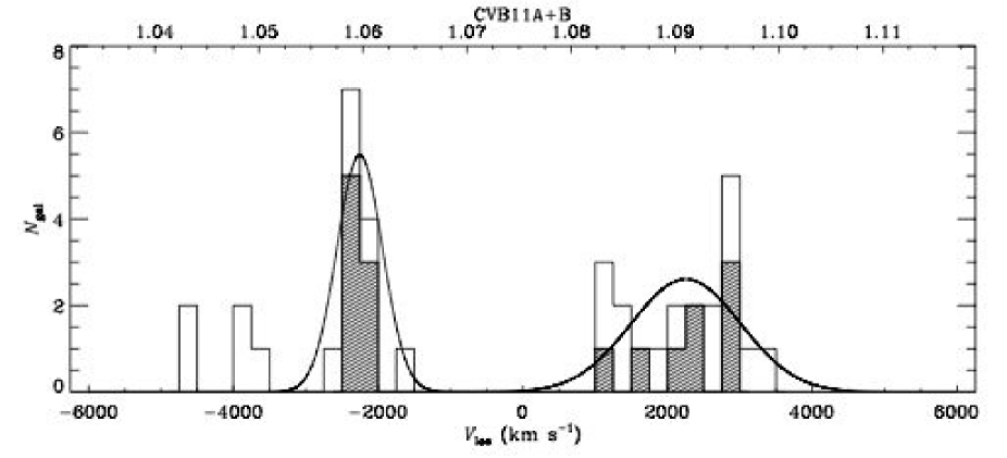
Figure 7: Velocity distributions of clusters CVB11A and CVB11B. The overplotted Gaussian functions are determined by $\overline{z}=1.0593\,\pm\,0.0003$ and $\sigma_{v}=316\,\pm\,166\,\rm km\,s^{-1}$ for CVB11A and $\overline{z}=1.091\,\pm\,0.001$ and $\sigma_{v}=650\,\pm\,95\,\rm km\,s^{-1}$ for CVB11B. The shaded bins are objects from the SXDF master list.

Using the publicly available software package XSPEC we fit a model spectral energy distribution to the X-ray spectrum. The model consists of two multiplied components: (i) the ‘mekal’ emission spectrum from diffuse hot gas based on the model calculations of Mewe and Kaastra (Mewe, Gronenschild & van den Oord, 1985; Mewe, Lemen & van den Oord, 1986; Kaastra, 1992) with iron emission line calculations by Liedahl, Osterheld & Goldstein (1995) and (ii) the ‘wabs’ photo-electric absorption model using Wisconsin cross-sections (Morrison and McCammon, 1983). The emission spectrum is determined by the temperature of the intracluster medium; the best-fitting value is $kT_{\rm X}=4\,\pm\,1.1\,\rm keV$ (rest-frame). The X-ray luminosity and velocity dispersion of CVB6 are exactly as expected according to the X-ray scaling relations for groups and clusters found by Xue & Wu (2000); the temperature is slightly higher than average but still within the scatter of the observed relations.

3.2 CVB11

3.2.1 Optical properties

Cluster CVB11 does not consist of a single redshift peak, but rather comprises two peaks at $z=1.06$ and $z=1.09$, with $\Delta V\sim 4500\,\rm km\,s^{-1}$. In this paper we designate the peak at $z=1.06$ with CVB11A, and the peak at $z=1.09$ with CVB11B. CVB11A has 9 confirmed cluster galaxies in our GMOS and DEIMOS data, and CVB11B has 11 cluster members. All 20 observed cluster galaxies of CVB11A and CVB11B are [O ii] emitters. The properties of the cluster galaxies are given in Table 7 in the Appendix.

Fig. 7 shows the velocity distributions of CVB11A and CVB11B, including the galaxies from the SXDF master list. The exact cluster redshift and velocity dispersions are calculated by using the bi-weighted mean of the galaxy redshifts and the ‘gapper’ estimate of the scale factor. Note that for CVB6 we used the bi-weighted estimate for the scale factor; the appropriate estimator needs to be chosen according to sample size, as discussed in Beers et al. (1990). We arrive at $\overline{z}=1.0593\,\pm\,0.0003$, $\sigma_{v}=316\,\pm\,166\,\rm km\,s^{-1}$ for CVB11A, and $\overline{z}=1.091\,\pm\,0.001$, $\sigma_{v}=650\,\pm\,95\,\rm km~{}s^{-1}$ for CVB11B. These velocity dispersions would, according to Eq. 1, relate to masses of $2.0\times 10^{13}$ and $1.7\times 10^{14}\rm\,M_{\odot}$ respectively. It is, however, unlikely that the latter is a true estimate of the cluster mass as the velocity distribution of cluster CVB11B from Fig. 7 does not appear to have achieved the Gaussian distribution expected in line-of-sight velocities of a virialised system. Unfortunately, the small sample size complicates the calculation of reliable statistics on the probability that the velocities are drawn from a Gaussion distribution. Using the method of Marshall et al. 1983, we execute a Bayesian likelihood test which is designed to choose the optimum model (Gaussian or flat velocity distribution) given the data. There is greater evidence for the flat model than the Gaussian model, however owing to the sparseness of the data the probability of the data being drawn from either distribution are only between 5 and 10%, which means neither can be confirmed or discarded reliably statistically.

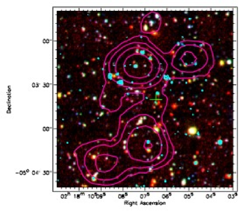
Figure 9: $Bi^{\prime}K$ image of the central $2^{\prime}$ of cluster CVB11A with X-ray and 1.4 GHz radio contours overlaid in purple and blue respectively. The three brightest X-ray point sources are background objects at $z=1.4$ (to the north), $z=1.3$ (to the northwest) and $z=3.1$ (to the south). The emission in the centre between these sources is identified by Finoguenov et al. as an extended source (green cross), possibly associated with the cluster. Data sources and contour levels are as in Fig. 5.

3.2.2 X-ray emission from the intracluster medium

The X-ray catalogue does not contain any extended sources that could be associated with cluster CVB11B. However, careful inspection of the X-ray emission at the central position of CVB11A shows excess flux between two bright point sources. Fig. 9 shows a three-colour image of the central $1^{\prime}$ of CVB11A with X-ray contours overlaid in purple and radio contours overlaid in blue. The three brightest X-ray point sources in this image are background sources at $z=1.3$, $z=1.4$, and $z=3.1$ with total fluxes of $0.5\,\pm\,0.2$, $0.5\,\pm\,0.3$, and $2.4\,\pm\,0.5\times 10^{-17}\rm\,W\,m^{-2}$ respectively. Finoguenov et al. (in preparation) apply a sophisticated point spread function removal technique to obtain fluxes for extended sources which are polluted by point sources. They indeed find an extended source at this position, with a flux of $1.9\,\pm\,0.5\times 10^{-18}\,\rm W\,m^{-2}$ in the 0.5 - 2.0 keV band. This would mean a luminosity of $L_{X}=1.2\times 10^{36}\,\rm W$ if the X-ray emission is associated with the cluster at $z=1.06$, which – according to the scaling relations of Xue & Wu (2000) – corresponds well to the estimated velocity dispersion.

3.3 CVB13

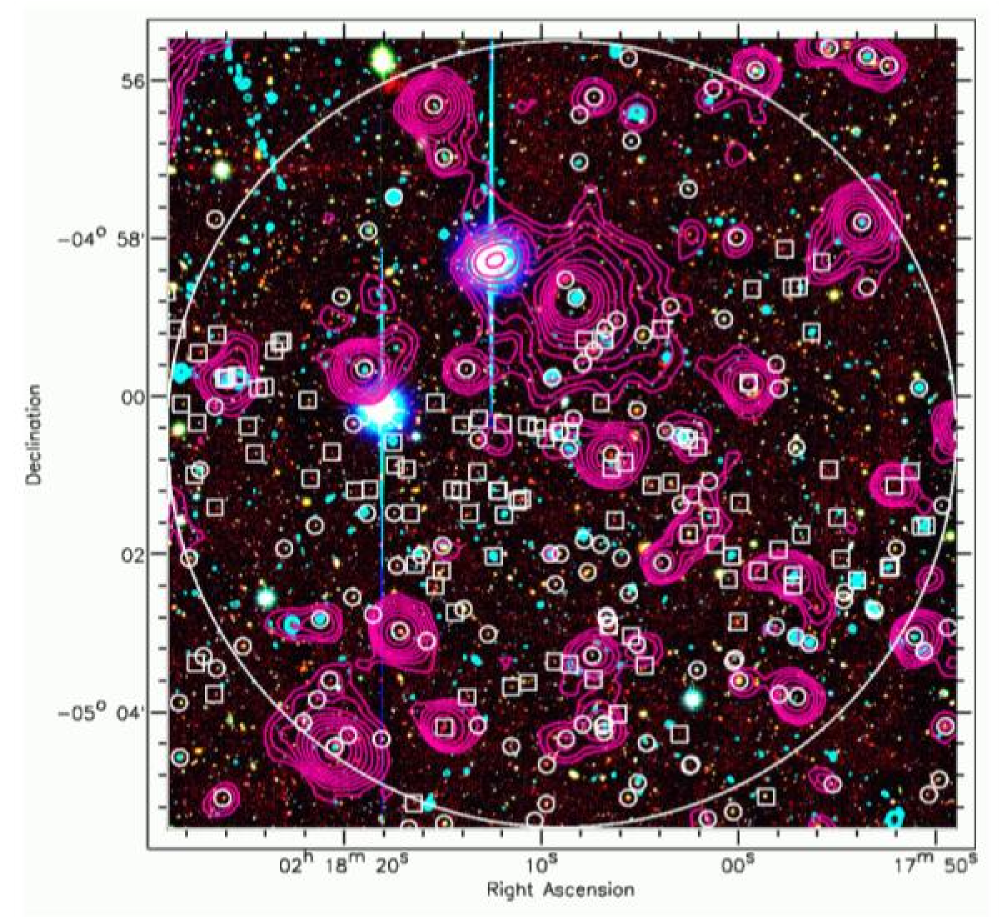
Figure 10: $Bi^{\prime}K$ image of cluster field CVB13. Symbols and contours are as in Fig. 8.

Cluster field CVB13 has been described in detail in VB07, where we discussed the two overdensities found in the DEIMOS data at $z=1.28$ and $z=1.45$. In this paper, we focus on the cluster at $z=1.28$ as the data on the second structure are sparse. We will refer to the cluster at $z=1.28$ as CVB13A. The table of cluster galaxies can be found in VB07, table 1: galaxies CVB13_2 to CVB13_11 are part of CVB13A.

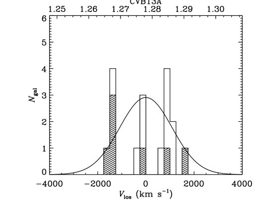
Figure 11: Velocity distributions of cluster CVB13A. The shaded bins are objects from the SXDF master list. The overplotted Gaussian function is determined by $\overline{z}=1.278,\pm\,0.002$, $\sigma_{v}=1092\,\pm\,141\,\rm km\,s^{-1}$. The data obviously deviate significantly from the Gaussian approximation.

We note that the combination of the DEIMOS and GMOS data with the SXDF spectroscopic master list yields a slightly different velocity distribution for CVB13A than the one presented in VB07, as is shown in Fig. 11. The mean redshift and velocity dispersion of the complete sample are $\overline{z}=1.278,\pm\,0.002$, $\sigma_{v}=1092\,\pm\,141\,\rm km\,s^{-1}$. Like CVB11B, the velocity distribution appears broad and non-Gaussian, and therefore the cluster is unlikely to be virialised. It is probable that the cluster comprises several merging sub-clumps; however the data do not support a good double Gaussian fit. We perform the same Bayesian likelihood test on the velocity distribution as on CVB11B (see Section 3.2.1); however owing to the small sample size we obtain the same inconclusive result.

4 The cluster AGN population

4.1 X-ray and radio sources

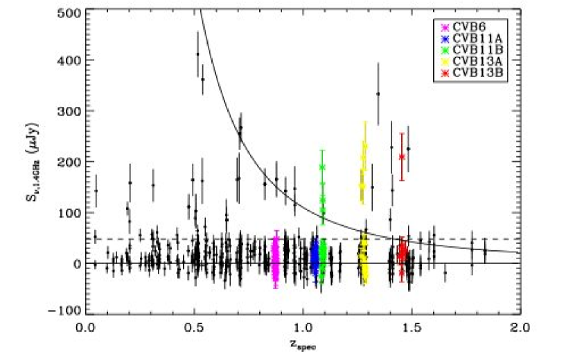
Figure 12: Radio flux density at 1.4 GHz versus redshift for all objects with a spectroscopic redshift in cluster fields CVB6, CVB11, and CVB13. Field galaxies are plotted in black, and cluster galaxies are plotted in blue for CVB6, green for CVB11A, yellow for CVB11B, and red for CVB13A. Note that two radio sources that are cluster members of CVB11B are not visible in this plot; their flux densities are $800$ and $2800\,\mu\rm Jy$. The solid curve shows the predicted radio flux density caused by a star-burst of $500\,\rm M_{\odot}\,yr^{-1}$ (total over all stellar masses); objects above the curve are assumed to be AGN. The dashed line is the average $5\sigma$ flux limit of the radio catalogue.

The deep X-ray and radio data in the SXDF combined with the optical spectroscopy allow us to investigate the AGN activity in the three cluster fields, and in particular in the four clusters themselves.

The X-ray catalogue contains 48 X-ray point sources in our fields, of which 42 (88 per cent) have an associated redshift in our spectroscopic catalogue. Visual inspections of X-ray-contour overlays show that despite $\sim 1.5^{\prime\prime}$ scale positional errors on the X-ray positions, there is almost always only one plausible candidate for follow-up spectroscopy. However in a few cases unambiguous identification is impossible.

The X-ray population at fluxes of $F_{\rm X}>10^{-18.5}\,\rm W\,m^{-2}$ in the 0.1 - 10 keV band consists predominantly of AGN, both obscured (up to $F_{\rm X}\sim 10^{-17}\,\rm W\,m^{-2}$) and unobscured (e.g. Barger et al. 2001, 2003; Szokoly et al. 2004). At lower fluxes, a population of star-forming galaxies emerges (Hornschemeier et al. 2000; Rosati et al. 2002; Norman et al. 2004). Other sources of X-ray emission from galaxies are X-ray binaries and the hot interstellar medium (ISM, e.g. Sivakoff, Sarazin & Irwin 2003). To determine whether the X-ray objects found in our fields could be star-forming galaxies, we calculate their rest-frame X-ray fluxes in the $0.1-10$ keV band. However, as the X-ray catalogue gives total fluxes in the $0.2-12$ keV band, we have to take both the redshifting of the spectrum ($k$-correction) and the difference in bands into account to obtain the correct fluxes. Guided by Ueda et al. (2003), we determine the corrections by assuming an X-ray SED of the form:

$${\rm SED}\,{\rm[keV]}=E^{-\Gamma}e^{\frac{E}{E_{c}}},$$ (2)

where $\Gamma=1.9$, and $E_{c}=500\rm\,keV$. The corrected flux in the $0.1-10$ keV band then becomes:

$$F_{\rm rest,0.1-10\,keV}=\frac{\int_{0.1}^{10}{\rm SED}\,dE}{\int_{(z+1)0.2}^{(z+1)12}{\rm SED}\,dE}F_{\rm obs,2-12\,keV}$$ (3)

The minimum flux in this band observed in our fields is $F_{\rm 0.1-10\,keV}=4.7\times 10^{-18}\,\rm W\,m^{-2}$, which implies the X-ray sources in our sample are not star-forming galaxies. To rule out contaminants by X-ray binaryies and the ISM, we follow the method of Sivakoff et al. (2008). We calculate the broadband X-ray luminosity in the 0.3 - 8.0 keV band, and compare with the $K_{S}$-band luminosity of the galaxies. We find our sources have X-ray luminosities in the range of $3\times 10^{42}<L_{\rm X,0.3-8.0}<4\times 10^{46}~{}\rm erg~{}s^{-1}$. The $K_{S}$-band luminosities are derived from the $K$-band luminosites from the Ultra Deep Survey (UDS), and band corrected by subtracting a value of 0.017 (Hewett et al. 2006); they range between $1\times 10^{10}$ and $2\times 10^{12}~{}\rm L_{K_{S},\odot}$. It appears the large X-ray luminosity of all our sources compared to their $K$-band luminosity rules out contamination by X-ray binaries and the ISM. We therefore can safely assume all of the objects in our sample are AGN.

The VLA A-array catalogue includes all sources with a flux greater than $5\sigma$, where $\sigma$ is the local noise; on average this means the sources have $S_{\rm 1.4\,GHz}\mathrel{\hbox{\hbox to0.0pt{\hbox{\lower 2.0pt\hbox{$\sim$}}\hss}\raise 2.0pt\hbox{$>$}}}50\,\rm\mu Jy$. This catalogue contains 87 sources within the three cluster fields, of which 40 have a spectroscopic redshift (46 per cent). Extragalactic radio sources fall into two main types of objects: star-forming galaxies and AGN. Generally the radio emission of the brightest sources is caused by an active nucleus, whereas the star-forming galaxies dominate the radio population at lower radio power. To distinguish between these two populations, we assume that the maximum total star-formation rate of a galaxy is $500\rm\,M_{\odot}\,yr^{-1}$ (at which Mauch & Sadler [2007] find that the space density of AGN is $\sim$ 20 higher than star-forming galaxies) and calculate the corresponding radio flux density at redshifts $0<z<2$ using the following relations from Condon (1992):

$${\rm SFR}_{\rm non-thermal}=\frac{P~{}{\rm[W\,Hz^{-1}]}}{5.3\times 10^{21}\,\nu^{-\alpha}},$$ (4)

$${\rm SFR}_{\rm thermal}=\frac{P~{}{[\rm W\,Hz^{-1}]}}{5.5\times 10^{20}\,\nu^{-0.1}}.$$ (5)

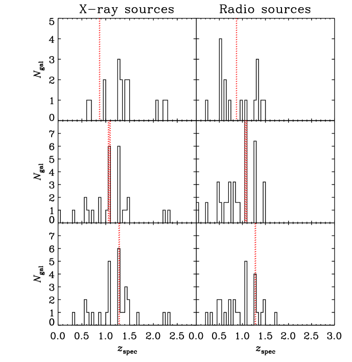
Figure 13: Redshift distribution of the radio sources and X-ray point sources in the cluster fields of CVB6 (top), CVB11 (middle), and CVB13 (bottom). The red shaded regions are within a velocity range of $\pm\,2000\,\rm km\,s^{-1}$ of the clusters.

Here $P$ is the radio power at frequency $\nu$ (1.4 GHz), and $\alpha\sim 0.8$ is the non-thermal spectral index. These equations determine the radio power caused by a star formation in stars of masses $\geq 5\,\rm M_{\odot}$ only; assuming a Salpeter IMF the star-formation rate in all stars is a factor of 5 higher. This means that the radio power limit for star-forming galaxies is $P_{\rm lim,\,1.4\,GHz}=5\times 10^{23}\,\rm W\,Hz^{-1}$. Fig. 12 shows the limiting radio flux density versus redshift with the flux densities of all our radio sources overplotted. These flux densities have been $k$-corrected to reflect the rest-frame 1.4 GHz radio power; for this we assume a spectral index of 0.8. All objects with a radio flux density greater than the limiting radio flux density are assumed to be AGN; from Fig. 12 we can see that all objects we find with a flux density $\geq 5\sigma$ at our clusters’ redshifts fall within this category.

4.2 The number density of active galaxies

The redshift distribution of the X-ray and radio sources is shown in Fig. 13 for each of the fields; note that a number of sources is included in more than one histogram due to the overlap of the cluster fields (see Fig.1).

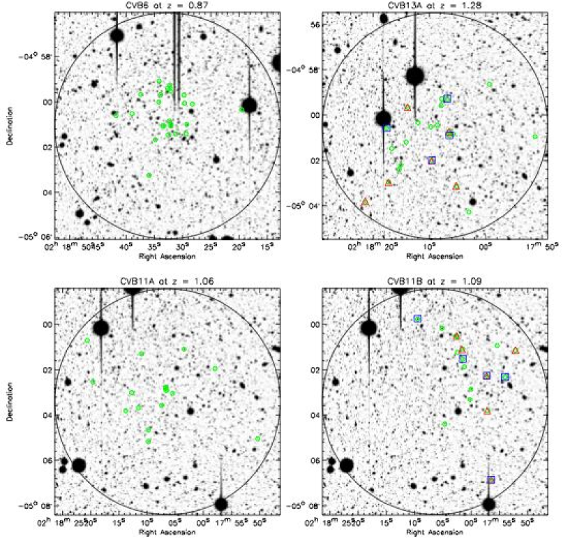
Figure 14: Cluster galaxies (green circles) and associated X-ray (red triangles) and radio (blue squares) AGN overlaid on $i^{\prime}$-band images of CVB6, CVB11A, CVB11B, and CVB13A. All objects marked by symbols are within $\pm\,2000\,\rm km\,s^{-1}$ of the cluster redshift. The black circle marks the $5^{\prime}$-radius field that was investigated. Note that there are no AGN associated with clusters CVB6 and CVB11A.

It is apparent from this figure that there are no radio sources nor X-ray point sources associated with cluster CVB6. For clusters CVB11A, CVB11B, and CVB13A we inspect the velocity range of $\pm\,2000\,\rm km\,s^{-1}$ around the cluster redshifts: any radio or X-ray point sources in the respective fields within this velocity interval are taken to be associated with the clusters. Cluster CVB11A also has no associated radio or X-ray point sources; CVB11B and CVB13A however both contain a number of X-ray and radio sources. The positions of the cluster galaxies, X-ray point sources, and radio sources are plotted for each cluster in Fig. 14. Table 1 lists the number of associated AGN per cluster. We note that the broadband X-ray luminosity limit for CVB6 and CVB11A is $2\times 10^{42}~{}\rm erg~{}s^{-1}$; this means we may be missing low-luminosity X-ray AGN of $L_{\rm X}\geq 10^{41}~{}\rm erg~{}s^{-1}$. However, the luminosity limits of CVB11B and CVB13 are even higher as they lie at greater redshift. Therefore, we would be missing the same or even larger fraction of AGN in these clusters and the lack of detected AGN in the lower-redshift clusters is not due to an observational bias.

Cluster	$N_{\rm gal}$	$N_{\textrm{X}-ray}$	$N_{\textrm{r}adio}$	$N_{\textrm{e}xp,\,X-ray}$	$N_{\textrm{e}xp,\,radio}$	$P(N_{\textrm{X}-ray}|N_{\textrm{e}xp})$	$P(N_{\textrm{r}adio}|N_{\textrm{e}xp})$
CVB6	25	0	0	0.92	0.15	$3.5\times 10^{-1}$	$7.0\times 10^{-1}$
CVB11A	14	0	0	0.90	0.16	$3.6\times 10^{-1}$	$6.9\times 10^{-1}$
CVB11B	16	6	5	0.90	0.16	$2.7\times 10^{-4}$	$1.0\times 10^{-5}$
CVB13A	18	5	4	0.85	0.15	$1.7\times 10^{-3}$	$1.0\times 10^{-5}$

Table 1: The numbers of AGN associated with the clusters in a field of $5^{\prime}$ radius, together with the expected numbers. The first column is the cluster ID, the second is the total number of spectroscopically confirmed cluster galaxies, and columns 3 and 4 are the number of X-ray and radio AGN respectively. Columns 5 and 6 show the numbers of expected X-ray and radio AGN if the inspected cluster fields were random background fields. Columns 7 and 8 are the probabilities that the number of observed AGN are caused by the background distribution of AGN.

We can calculate the number of expected X-ray and radio AGN within the probed volume, by integrating over the respective luminosity functions. For the X-ray sources, we use the Hard X-ray Luminosity Function (HXLF) in the 2-10 keV band from Ueda et al. (2003). This is a luminosity-dependent density evolution model of the following form:

$$d\Phi=A\Bigl{\{}\Bigl{(}\frac{L_{\rm X}}{L^{*}}\Bigr{)}^{\gamma_{1}}+\Bigl{(}\frac{L_{\rm X}}{L^{*}}\Bigr{)}^{\gamma_{2}}\Bigr{\}}^{-1}e(z)d\log(L_{\rm X}),$$ (6)

where $\Phi$ is the number density per cubic Mpc, and $e(z)$ is the evolution factor. The values of the constant parameters in this and the following two equations are given in Ueda et al. (2003). The evolution factor is given by:

$$e(z)=\left\{\begin{array}[]{lr}(1+z)^{p_{1}}&z<z_{c}(L_{\rm X})\\ e(z_{c})\Bigl{(}\frac{1+z}{1+z_{c}(L_{\rm X})}\Bigr{)}^{p_{2}}&z\geq z_{c}(L_{\rm X})\\ \end{array}\right.$$ (7)

Here $z_{c}$ is the cut-off redshift above which the evolution terminates, which is dependent on the X-ray luminosity in the following way:

$$z_{c}(L_{\rm X})=\left\{\begin{array}[]{lr}z_{c}^{*}&L_{\rm X}\geq L_{\rm a}\\ z_{c}^{*}\Bigl{(}\frac{L_{\rm X}}{L_{\rm a}}\Bigr{)}^{\alpha}&L_{\rm X}<L_{\rm a}\\ \end{array}\right.$$ (8)

We calculate the minimum observed flux in the $2-10$ keV band, applying the corrections of Eq. 3, and obtain $F_{\rm min,\,2-10\,keV}=4.1\times 10^{-19}\,\rm W~{}m^{-2}$. Converting this to a luminosity, integrating Eq. 6 from this value upwards, and multiplying by the volume given by the circular field of $5^{\prime}$-radius and $\Delta V=4000\,\rm km\,s^{-1}$ gives on average one expected X-ray source in a random volume of this size. Taking the completeness into account, this number is reduced to 0.9.

The radio luminosity function consists of three components: (i) a luminosity function for radio-loud AGN (Willott 2001); (ii) a radio luminosity function for radio-quiet AGN derived from the X-ray luminosity function from Ueda et al. (2003) and converted to radio using the relations set out in Brinkmann et al. (2000); (iii) a luminosity function for star-forming galaxies derived from infrared observations (Yun, Reddy & Condon 2001), taking into account the redshift evolution observed in submillimetre source counts (Blain 1999). Combining all three, integrating from our luminosity limit upwards, and accounting for our completeness, yields an average expected number of 0.2 radio sources in our cluster fields if they were random fields (see Jarvis & Rawlings 2004 and Wilman et al. 2008 for a detailed description of the method used). The exact expected number of AGN per cluster are given in Table 1. We use Poissonian low-number statistics to calculate the probability that the observed numbers of AGN are fluctuations of the expected background model. These numbers are also listed in Table 1; we conclude that the observed numbers of X-ray and radio sources in CVB11B and CVB13A are $3-5\sigma$ away from the expected numbers, which indicates that the AGN in these fields are clustered to a highly-significant level. The absence of AGN in CVB6 and CVB11A is consistent with the AGN population being no different in these clusters than in the field.

5 Discussion

To inspect the two-dimensional clustering of the AGN associated with CVB11B and CVB13A, we calculate the $A/A_{\rm max}$ statistic for both the X-ray and the radio sources. This statistic is the ratio of the average area, in which the AGN occur, to the maximum investigated area. For each AGN the area is defined as the circle with a radius determined by the distance of the AGN to the cluster centre. $A_{\rm max}$ is the area of the circle with a radius of 5^′. If the AGN are randomly distributed over the field, the value of $A/A_{\rm max}$ is 0.5; a value $<0.5$ indicates clustering in right ascension and declination. The result is shown in Table 2; evidently, the AGN are clustered within a smaller field than the total $5^{\prime}$-radius fields. This is not surprising, as the $r_{200}$ virial radius of a cluster such as CVB6 ($M_{200}=1.6\times 10^{14}\,\rm M_{\odot}$) is only 1.3 Mpc in proper coordinates, whereas a field of $5^{\prime}$ radius would correspond to 2.4 Mpc at $z=1.0$.

Cluster	$A_{\textrm{X}-ray}/A_{\textrm{m}ax}$	$A_{\textrm{r}adio}/A_{\textrm{m}ax}$	$A_{\textrm{A}GN}/A_{\textrm{m}ax}$
CVB11B	0.2$\,\pm\,$0.2	0.3$\,\pm\,$0.3	0.2$\,\pm\,$0.2
CVB13A	0.3$\,\pm\,$0.3	0.1$\,\pm\,$0.3	0.2$\,\pm\,$0.2

Table 2: The $A/A_{\rm max}$ statistic for both the X-ray and the radio sources associated with clusters CVB11B and CVB13A. Columns 2 and 3 show the statistic for X-ray and radio sources respectively, and column 4 is the combined statistic after removal of coincident detections.

Cluster	$N_{\textrm{X}-ray}$	$N_{\textrm{r}adio}$	$N_{\textrm{e}xp,\,X-ray}$	$N_{\textrm{e}xp,\,radio}$	$P(N_{\textrm{r}adio}|N_{\textrm{e}xp})$	$P(N_{\textrm{r}adio}|N_{\textrm{e}xp})$
CVB6	0	0	7.6	1.3	$5.1\times 10^{-4}$	$2.6\times 10^{-1}$
CVB11A	0	0	5.6	0.98	$3.0\times 10^{-3}$	$3.3\times 10^{-1}$
CVB11B	5	3	5.3	0.96	$6.1\times 10^{-1}$	$7.2\times 10^{-2}$
CVB13A	2	4	3.9	0.70	$2.5\times 10^{-1}$	$5.6\times 10^{-3}$

Table 3: The numbers of AGN associated with the clusters within a radius of $r_{200}$ of CVB6 ($2.6^{\prime}$), together with the expected numbers of AGN assuming a cluster with an overdensity of factor 200. The first column is the cluster ID, and columns 2 and 3 are the number of X-ray and radio AGN respectively. Columns 4 and 5 show the numbers of expected X-ray and radio AGN, assuming their clustering traces the mass overdensity. Columns 6 and 7 are the probabilities that the number of observed AGN are caused by an overdensity of factor 200.

As CVB11B and CVB13A do not appear to be virialised, we cannot calculate a virial mass – and thus radius – from the velocity dispersion. The number of galaxies found in the clusters suggest however that they are of lower mass than CVB6 and therefore confined to a smaller radius. On the other hand, if the clusters are not virialised yet, they could occupy a larger volume than virialised systems of the same mass. We therefore assume these effects cancel out roughly, and examine the AGN of CVB11B and CVB13A within the virial radius $r_{200}=1.3\rm\,Mpc$ (proper coordinates) of CVB6, which corresponds to $2.6^{\prime}$ at the redshift of the two clusters. We determine the number of AGN in these new fields and show them in Table 3. Further, we recalculate the number of expected X-ray and radio sources, this time assuming a cluster environment (in proper coordinates) with a total overdensity of a factor of 200 (implied by the definition of $r_{200}$). Using these new numbers, we can establish the probability that the number of observed AGN is caused by the overdensity in the background distribution. These numbers are also given in Table 3. An interesting result emerges: the lack of X-ray sources in CVB6 and CVB11A is significant at a level of $\geq 3\sigma$, whereas the lack of radio sources is not significant. Contrarily, the number of X-ray sources in CVB11B and CVB13A are consistent with being caused by an overdensity of factor 200, whereas the radio sources appear to be even more clustered than that. In fact, the numbers suggest the radio sources are a factor 3 - 6 more clustered than the X-ray sources.

In summary, we have presented evidence that the AGN population of clusters appears to change fundamentally during the evolution of the cluster, although our conclusions are limited by small number statistics. Clusters CVB11B and CVB13A seem to be in a state of pre-virialisation, as can be derived from their velocity distributions. They show a number of associated AGN far above the background level, and consistent with an overdensity comparable with the total mass overdensity, although the radio galaxies appear to be even more heavily clustered. Clusters CVB6 and CVB11A are in a later evolutionary stage, and both have an extended X-ray detection. CVB6 is the best example of this: the X-ray properties and velocity distribution all lie neatly on normal cluster relations. These two clusters have few, if any, associated AGN, which means that the AGN activity is less or equal to that of the galaxy field. It is possible that as the cluster virialises, AGN activity is extinguished, leaving the clusters quiescent.

A potential explanation for this observed phenomenon is as follows. X-ray AGN contain a supermassive black hole in their galactic nucleus which accretes gas at a high rate. This means a large amount of fuel is needed on small scales, which could be caused by a galaxy-galaxy merger (e.g. Barnes & Hernquist 1996). Pre-virialised clusters most likely consist of merging sub-groups with low internal velocity dispersions, which allows galaxy mergers. The galaxies in virialised clusters however have high relative velocities, which suppresses the galaxy merger rate (e.g. Giovanelli & Haynes 1985). Hence the X-ray AGN fraction is much lower in virialised clusters than in systems which are in an earlier evolutionary stage.

Radio AGN are probably caused by rapidly spinning supermassive black holes in the nuclei of massive galaxies, created my the merger of two nuclear black holes of similar mass (Wilson & Colbert 1995). Objects at a given radio luminosity can have a wide range of accretion rate of the black hole. The high-accretion sources are identical to the X-ray sources; indeed we observe some overlap between our X-ray and radio AGN. In a cluster environment galaxy-galaxy harassment can boost the accretion rate (Moore et al. 1996), which increases the radio power (e.g. Willottt et al. 1999). Also, the luminosity of a radio jet can be increased by higher intergalactic gas densities, as the jet encounters a denser medium (e.g. Prestage & Peacock, 1988; Daly, 1995). The intracluster medium both in virialised and pre-virialised clusters is generally denser than in a field environment; the galaxy interaction is higher in pre-virialised systems for the same reason as for the galaxy merger rate.

Hopkins et al. (2005) show that the lifetime of a luminous quasar caused by a merger is expected to be of the order of $\sim 10^{7}\,$yr ($B$-band luminosity greater than $10^{11}\,\rm L_{\odot}$) to $10^{9}\,$yr ($B$-band luminosity greater than $10^{9}\,\rm L_{\odot}$) when taking into account attenuation by obscuring material, with an intrinsic lifetime of $\sim 10^{8}\,-10^{9}$yr. This means that if no new AGN are triggered after virialisation, the cluster would be left quiescent after this length of time. Furthermore, during virialisation it is likely that one big radio AGN is triggered, that could shut down all AGN activity henceforward in a cluster (Rawlings & Jarvis, 2004). This is a further explanation for the lack of activity in virialised clusters such as CVB6 and CVB11A, where this event may already have happened, whereas CVB11B and CVB13A have not encountered this phenomenon yet.

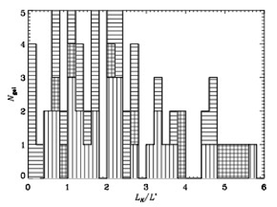
Figure 15: The luminosity in terms of the passively evolving $L^{*}$ for radio (vertical hatching) and X-ray (horizontal hatching) AGN. The cross-hatched bins are AGN that show both X-ray and radio emission.

If the above scenario is valid, we expect the galaxy hosts of the AGN to be more massive than normal galaxies. The prediction for X-ray AGN is $\sim 2L^{*}$, whereas it is slightly higher for radio galaxies ($2-3L^{*}$) as the spinning black holes appear to be found only in the most-massive objects (e.g. Dunlop et al. 2003). Fig. 15 shows the $K$-band luminosity histogram of all X-ray and radio AGN in our fields (at all redshifts) expressed as a fraction of $L^{*}$ (assumed to be passively evolving, with $M_{K}^{*}=-24.18$ at $z=0$ [Cole et al. 2001, corrected for cosmology and difference in $K$-bands]), which is the luminosity at which the break in the galaxy luminosity function occurs. It appears that the radio galaxies (vertically hatched bins) are slightly more massive than the X-ray galaxies (horizontally hatched bins). The median luminosity for the X-ray sources is $L_{K}=1.7\,\pm\,0.7\,L^{*}$, whereas the for radio sources we find a median of $L_{K}=2.3\,\pm\,0.1\,L^{*}$. Nonetheless we need to bear in mind that the higher measured AGN luminosities could instead be due to an observational selection bias as, given the same Eddington accretion rate, the more powerful AGN reside in more massive galaxies, which would be more easily detected.

If the observed distribution of luminosities reflects the true AGN luminosity distribution, this would support the hypothesis described above for AGN fractions residing in clusters of different evolutionary stages. However, we are dealing with low-number statistics and a more comprehensive sample is needed to confirm our findings. This is of particular importance, as Martini et al. (2007) show that there is significant variation in the X-ray selected AGN fraction between clusters at lower redshift. Ruderman & Ebeling (2005) find an overdensity of X-ray AGN in 51 massive clusters at $0.3<z<0.7$. Their sample shows an excess in the centre of the clusters, likely to be caused by the central cluster galaxy, followed by a depletion in the intermediate regions and a secondary excess at a distance greater than 2.5 Mpc. The latter is attributed to galaxy merging and interaction during infall into the cluster. At first glance, this is at odds with our findings, as we do not find an excess in our virialised clusters. However, our sample differs significantly from Ruderman & Ebeling’s, as our clusters are less massive and at much higher redshift. These circumstances could cause the central cluster galaxy to not yet have been activated if it is triggered in a later stage of the cluster’s evolution. Furthermore, our field of view of $5^{\prime}$ corresponds to 2.4 Mpc at $z=1$, meaning that we do not probe the outer regions in which Ruderman & Ebeling find their secondary excess. Their conclusion that this is caused by merging galaxies is actually in agreement with our findings for our non-virialised clusters. It is evident that to link all studies of AGN in clusters, we will need large cluster samples imaged in both the radio and X-ray regime at a range of redshifts. Future deep, wide-field optical/infrared surveys, such as the Visible and Infrared Survey Telescope for Astronomy (VISTA) Deep Extragalactic Observations Survey (VIDEO), coupled with X-ray and radio observations, will be vital to acquire a large sample of clusters and AGN at $z>1$.

6 Acknowledgments

The authors would like to thank Doi, Morokuma, Miyazaki, Saito, Yamada, Satoshi, Smail, and Croom for sharing their redshifts in the SXDF master list. CVB acknowledges support from STFC in the form of a postdoctoral felloship. This paper is partly based on observations obtained at the Gemini Observatory, which is operated by the Association of Universities for Research in Astronomy, Inc., under a cooperative agreement with the NSF on behalf of the Gemini partnership: the National Science Foundation (United States), the Science and Technology Facilities Council (United Kingdom), the National Research Council (Canada), CONICYT (Chile), the Australian Research Council (Australia), Minist rio da Ci ncia e Tecnologia (Brazil) and SECYT (Argentina). Some of the data presented herein were obtained at the W.M. Keck Observatory, which is operated as a scientific partnership among the California Institute of Technology, the University of California and the National Aeronautics and Space Administration. The Observatory was made possible by the generous financial support of the W.M. Keck Foundation. The authors wish to recognize and acknowledge the very significant cultural role and reverence that the summit of Mauna Kea has always had within the indigenous Hawaiian community. We are most fortunate to have the opportunity to conduct observations from this mountain.

Appendix A GMOS targets

ID	$z_{\rm phot}$	RA	Dec.	PA	$N_{\rm P1}$	$N_{\rm P2}$	$N_{\rm P3}$	$N_{\rm P1,MOS}$	$N_{\rm P2,MOS}$	$N_{\rm P3,MOS}$
		[h m s]	[∘ ′ ′′]	[∘]
CVB6	0.76 $\pm$ 0.12	02 18 32.7	-05 01 04	335	44	139	95	15	16	5
CVB7	0.78 $\pm$ 0.06	02 19 03.5	-04 42 33	290	17	61	89	6	14	8
CVB8	0.79 $\pm$ 0.07	02 17 54.0	-05 02 54	310	15	63	99	10	13	7
CVB9	0.80 $\pm$ 0.06	02 17 21.4	-05 11 30	225	16	102	91	11	15	3
CVB11	0.95 $\pm$ 0.11	02 18 06.7	-05 03 13	90	66	187	71	17	12	1

Table 4: Targeted cluster candidates. The IDs (column 1) and photometric redshifts (column 2) are from VB06. The RA and Dec (column 3 and 4) are the coordinates of the telescope pointing and column 5 is the position angle of the instrument (east from north). Columns 6, 7, and 8 give the number of target galaxies of priority 1, 2, and 3 respectively, and columns 9, 10, and 11 show the number of galaxies of each priority included in the MOS mask.

ID	$z_{\rm phot}$	$z_{\rm spec}$	$N_{\rm gal}$	$N_{\rm gal}$
			($\Delta z=0.02$)	($\Delta z=0.04$)
CVB6	0.76 $\pm$ 0.12	0.87	7	7
CVB7	0.78 $\pm$ 0.06	0.91	4	5
CVB9	0.80 $\pm$ 0.06	0.92	6	12
CVB11	0.95 $\pm$ 0.11	1.05	6	8

Table 5: Spectroscopic redshifts of the five clusters targeted with GMOS and DEIMOS. The spectroscopic redshift given in column 3 is the peak of the redshift distribution in Figs. 16. For a further discussion on the exact cluster redshifts of CVB6 and CVB11, see Section 3. The number of galaxies within bins of $\Delta z=0.2$ and $\Delta z=0.4$ of the redshift peak is given in columns 4 and 5 respectively.

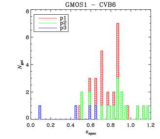
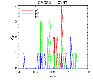
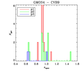
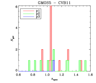
Figure 16: Distributions of the spectroscopic redshifts in each of the GMOS fields, targeting clusters CVB6, CVB7, CVB9, and CVB11. The three initial priorities of the targets (see Section 2) are colour-coded: red is priority 1, green is priority 2, and blue is priority 3.

Appendix B Photometric versus spectroscopic redshifts

We have matched our spectroscopic sample with our photometric redshift catalogue (see VB06); the resulting diagram of $z_{\rm phot}$ versus $z_{\rm spec}$ is shown in Fig. 17. Overplotted is the line for which $z_{\rm phot}=z_{\rm spec}$. It is apparent that most objects lie along this line, however there are outliers, most of which have photometric redshifts that are greatly overestimated. Closer inspection of these objects reveals that the majority are AGN for which our photometric redshift code is ill-suited as it does not include the appropriate spectral energy distribution templates. A histogram of the difference between the two redshift determinations, scaled with redshift, is plotted in Fig. 18. Overplotted is a Gaussian fit to the data; the mean difference is $(z_{\rm phot}-z_{\rm spec})/(1+z_{\rm spec})=-0.02$. The error on the photometric redshift is $\sigma_{z}/(1+z_{\rm spec})=0.056$.

A more subtle effect seen in Fig. 17 is a ‘stepping’ of the photometric redshift along the $z_{\rm phot}=z_{\rm spec}$ line: this is caused by the spikes in the photometric redshift distribution. This is shown more clearly in Fig. 19; here the difference between the two redshift determinations scaled with redshift is plotted versus the spectroscopic redshift. It is evident that the redshift spikes mainly comprise galaxies with spectroscopic redshifts slightly deviating from the spike redshift, as opposed to obvious outliers. This means that the redshifts of galaxies just below the spike are slightly overestimated, and vice versa for galaxies with slightly higher redshifts. This explains why the redshifts of the clusters targeted with spectroscopy all seemed to be underestimated by our algorithm (see Table 5), as they lie at redshift $\sim 0.9$ which is just above the most prominent redshift spike at $\sim 0.7$.

Figure 17: Photometric redshift versus spectroscopic redshift for all galaxies in our sample at $z_{\rm spec}\leq 2$. Overplotted for reference is the line for which $z_{\rm phot}=z_{\rm spec}$.

Figure 18: Histogram of the difference between the photometric and spectroscopic redshifts. Overplotted is a Gaussian function fitted to the distribution. The mean difference $(z_{phot}-z_{\rm spec})/(1+z_{\rm spec})$ is -0.02. The error on the photometric redshift is $\sigma_{z}/(1+z_{\rm spec})=0.056$.

Figure 19: The difference between the photometric and spectroscopic redshifts versus $z_{\rm spec}$

Appendix C Tables of cluster members

ID	RA	Dec.	$z_{\rm spec}$	$F_{\rm[OII]}$	$L_{\rm[OII]}$	$EW_{0}$
	[h m s]	[∘ ′ ′′]		[$10^{-20}~{}\rm W~{}m^{-2}$]	[$10^{34}~{}\rm W$]	[$\rm\AA$]
CVB6_1	02:18:32.356	-05:00:51.23	0.86476	-	-	-
CVB6_2	02:18:33.370	-05:01:03.87	0.86603	-	-	-
CVB6_3	02:18:32.543	-05:01:27.26	0.86626	-	-	-
CVB6_4	02:18:29.772	-04:59:42.89	0.86976	1.11	0.41	23
CVB6_5	02:18:34.818	-05:01:40.71	0.87001	-	-	-
CVB6_6	02:18:35.391	-05:00:58.15	0.87052	-	-	-
CVB6_7	02:18:32.239	-04:59:15.39	0.87056	1.50	0.56	5
CVB6_8	02:18:32.157	-04:59:24.70	0.87060	0.90	0.33	25
CVB6_9	02:18:37.447	-04:59:40.90	0.87064	1.59	0.59	42
CVB6_10	02:18:28.275	-05:00:05.84	0.87155	3.26	1.21	20
CVB6_11	02:18:35.286	-05:03:36.13	0.87162	2.87	1.07	5
CVB6_12	02:18:32.971	-05:00:51.11	0.87165	0.90	0.34	4
CVB6_13	02:18:29.653	-05:00:03.85	0.87180	1.45	0.54	25
CVB6_14	02:18:32.665	-04:59:24.59	0.87222	7.59	2.83	47
CVB6_15	02:18:32.789	-04:59:35.14	0.87294	3.57	1.33	36
CVB6_16	02:18:29.384	-05:01:24.56	0.87356	1.02	0.38	34
CVB6_17	02:18:41.821	-05:00:36.87	0.87499	7.40	2.78	54
CVB6_18	02:18:33.883	-04:59:41.42	0.87663	3.78	1.43	11
CVB6_19	02:18:38.941	-05:00:31.54	0.87753	-	-	-
CVB6_20	02:18:33.504	-05:01:03.57	0.87903	-	-	-

Table 6: Properties of the cluster galaxies of CVB6. Column 1 states the ID and the RA and Dec are given in columns 2 and 3. Column 4 is the heliocentric redshift; for the non-[O ii] emitters this is measured via a cross-correlation technique with an estimated average error of $\sim 2\times 10^{-4}$. For the [O ii] emitters the redshift and line flux (column 5) are taken from a double Gaussian fit to the [O ii] 3727 Å line profile, with an average error of $\sim 5\times 10^{-5}$ in redshift, and $\sim 1\times 10^{-21}\rm W\,m^{-2}$ in flux. The line luminosity is shown in column 6, and column 7 is the rest-frame equivalent width.

ID	RA	Dec.	$z_{\rm spec}$	$F_{\rm[OII]}$	$L_{\rm[OII]}$	$EW_{0}$
	[h m s]	[∘ ′ ′′]		[$10^{-20}~{}\rm W~{}m^{-2}$]	[$10^{34}~{}\rm W$]	[$\rm\AA$]
CVB11A_1	02:18:12.399	-05:03:57.02	1.04765	1.31	0.77	26
CVB11A_2	02:18:11.004	-05:01:18.16	1.04799	2.99	1.75	31
CVB11A_3	02:18:20.645	-05:00:42.44	1.04897	1.83	1.08	80
CVB11A_4	02:18:04.326	-05:03:40.73	1.05744	0.90	0.54	14
CVB11A_5	02:18:04.760	-05:03:24.71	1.05865	4.03	2.42	49
CVB11A_6	02:18:05.479	-05:03:02.34	1.05874	8.98	5.40	63
CVB11A_7	02:17:57.969	-05:01:56.82	1.06013	3.53	2.13	57
CVB11A_8	02:18:42.363	-05:01:31.55	1.06311	11.9	7.27	69
CVB11B_9	02:18:27.599	-05:01:00.03	1.08248	1.88	1.20	29
CVB11B_1	02:18:27.599	-05:01:00.03	1.08295	1.11	0.71	9
CVB11B_2	02:18:02.998	-05:04:16.71	1.08416	1.44	0.92	19
CVB11B_3	02:18:02.509	-05:00:32.97	1.08440	1.12	0.72	3
CVB11B_4	02:17:57.227	-05:02:16.30	1.08795	5.85	3.77	2
CVB11B_5	02:18:01.459	-05:01:32.00	1.09003	5.10	3.30	9
CVB11B_6	02:18:00.503	-05:02:19.25	1.09231	1.64	1.07	11
CVB11B_7	02:18:24.556	-05:00:43.68	1.09276	3.83	2.49	33
CVB11B_8	02:18:01.169	-05:01:52.69	1.09441	2.73	1.78	137
CVB11B_9	02:17:55.399	-05:00:55.99	1.09472	4.51	2.95	56
CVB11B_10	02:17:52.096	-05:01:08.37	1.09559	1.38	0.90	12
CVB11B_11	02:17:53.995	-05:02:20.13	1.09785	3.34	2.20	66

Table 7: Properties of the cluster galaxies of CVB11A and CVB11B. Columns are as in Table 6.

References

- (1) Barnes J. E., Hernquist L., 1996, ApJ, 471, 115
- (2) Barger A. J., Cowie L. L., Mushotzky R. F, Richards E. A., 2001, AJ, 121, 662
- (3) Barger A. J. et al., 2003, AJ, 126, 632
- (4) Beers T. C., Flynn K., Gebhardt K., 1990, AJ, 100, 32
- (5) Best P. N., 2000, MNRAS, 317, 720
- (6) Blain A. W., 1999, MNRAS, 309, 955
- (7) Brinkmann W., Laurent-Muehleisen S. A., Voges W., Siebert J., Becker R. H., Brotherton M. S., White R. L., Gregg M. D., 2000, A&A, 356, 445
- (8) Bruzual G., Charlot S., 2003, MNRAS, 344, 1000
- (9) Cole S. et al., 2001, MNRAS, 326, 255
- (10) Condon J. J., 1992, ARA&A, 30, 575
- (11) Daly R. A., 1995, ApJ, 454, 480
- (12) Dunlop J. S., McLure R. J., Kukula M. J., Baum S. A., O’Dea C. P., Hughes D. H., 2003, MNRAS, 340, 1095
- (13) Evrard A. E., 2008, ApJ, 672, 122
- (14) Fabian A. C., Celotti A., Erlund M. C., 2006a, MNRAS, 373L, 16
- (15) Foucaud S. et al., 2007, MNRAS, 376, L20
- (16) Furusawa H. et al, 2008, MNRAS, 176, 1
- (17) Giovanelli R., Haynes M. P., 1985, AJ, 90, 2445
- (18) Hewett P. C., Warren S. J., Legget S. K., Hodgkin S. T., 2006, MNRAS, 367, 454
- (19) Hill G. J. & Lilly S. J., 1991, ApJ, 367, 1
- (20) Hook I., Jørgensen I., Allington-Smith J. R., Davies R. L., Metcalfe N., Murowinski R. G., Crampton D., 2004, PASP, 116, 425
- (21) Hopkins P. F., Hernquist L., Martini P., Cox T. J., Robertson B., Di Matteo T., Springel V., 2005, ApJ, 625, L71
- (22) Hornschemeier A. E. et al., 2000, ApJ, 541, 49
- (23) Ivison R. J. et al., 2007, MNRAS,380, 199
- (24) Jarvis M. J., Rawlings S., 2004, NewAR, 48, 1173
- (25) Kaastra J. S., 1992, An X-Ray Spectral Code for Optically Thin Plasmas (Internal SRON-Leiden Report, updated version 2.0)
- (26) Liedahl, D. A., Osterheld, A. L., and Goldstein, W. H. 1995, ApJL, 438, 115
- (27) Martini P., Kelson D. D., Mulchaey J. S., Trager S. C., 2002, ApJ, 576, L109
- (28) Martini P., Kelson D. D.,, Kim E., Mulchaey J. S., Athey A. A., 2006, ApJ, 644, 116
- (29) Martini P., Mulchaey J. S., Kelson D. D., 2007, ApJ, 664, 761
- (30) Mauch T., Sadler E., 2007, MNRAS, 375, 931
- (31) Mewe R., Gronenschild E. H. B. M., van den Oord G. H. J., 1985, A&AS, 62, 197
- (32) Mewe R., Lemen J. R., van den Oord, G. H. J., 1986, A&AS, 65, 511
- (33) Miller C. J., Nichol R. C., G mez P. L., Hopkins A. M., Bernardi B., 2003, ApJ, 597, 142
- (34) Moore B, Katz N., Lakt G., Dressler A., Oemler A., 1996, Nature, 379, 613
- (35) Morrison R., McCammon D., 1983, ApJ 270, 119
- (36) Norman C. et al., 2004, ApJ, 607, 721
- (37) Prestage R. M., Peacock J. A., 1988 MNRAS, 230, 131
- (38) Rawlings S., Jarvis M. J., 2004, MNRAS, 355L, 9
- (39) Rosati P. et al., 2002, ApJ, 566, 667
- (40) Ruderman J. T., & Ebeling H., 2005, ApJ, 623, L81
- (41) Scannapieco E. & Oh P., 2004, AAS, 205, 1499
- (42) Simpson C. et al., 2006, MNRAS, 372, 741
- (43) Sivakoff G. R, Sarazin C. L., Irwin J. A., 2003, ApJ, 599, 218
- (44) Sivakoff G. R., Martini P., Zabludoff A. I., Kelson D. D., Mulchaey J. S., 2008, ApJ, 682, 803
- (45) Szokoly G. P. et al., 2004, ApJS, 155, 271
- (46) Ueda Y., Akiyama M., Ohta K., Miyaji T., 2003, ApJ, 598, 886
- (47) Van Breukelen C. et al., 2006, MNRAS, 373L, 26
- (48) Van Breukelen C. et al., 2007, MNRAS, 382, 971
- (49) Venemans B. et al., 2002, ApJ, 569L, 11
- (50) Watson M. G., Ueda Y., Akiyama M., Sekiguchi K. and the SXDS Collaboration, 2004, BAAS, 36, 1202 Smith A., 2000, in Minh Y. C., van Dishoeck E. F., eds, Proc. IAU Symp. 197, Astrochemistry: from molecular clouds to planetary systems. Astron. Soc. Pac., San Francisco, p. 210
- (51) Watson M. G et al., 2008, preprint (astro-ph0807.1067)
- (52) Willott C. J., Rawlings S., Blundell K. M., Lacy M., 1999, MNRAS, 309, 1017
- (53) Willott C. J., Rawlings S., Blundell K. M., Lacy M., Eales S. A., 2001, MNRAS, 322, 536
- (54) Wilman R. J., MNRAS, 388, 1335
- (55) Wilson A. S., Colbert E. J. M., 1995, ApJ, 438, 62
- (56) Xue Y.-J., Wu X.-P., 2000, ApJ, 538, 65
- (57) Yamada T. et al, 2005, ApJ, 634, 861
- (58) Yun M. S., Reddy N. A., Condon J. J., 2001 ApJ, 554, 803