A Faithful Semantics for
Generalised Symbolic Trajectory Evaluation

Abstract.

Generalised Symbolic Trajectory Evaluation (GSTE) is a high-capacity formal verification technique for hardware. GSTE is an extension of Symbolic Trajectory Evaluation (STE). The difference is that STE is limited to properties ranging over finite time-intervals whereas GSTE can deal with properties over unbounded time.

GSTE uses abstraction, meaning that details of the circuit behaviour are removed from the circuit model. This improves the capacity of the method, but has as down-side that certain properties cannot be proven if the wrong abstraction is chosen.

A semantics for GSTE can be used to predict and understand why certain circuit properties can or cannot be proven by GSTE. Several semantics have been described for GSTE by Yang and Seger. These semantics, however, are not faithful to the proving power of GSTE-algorithms, that is, the GSTE-algorithms are incomplete with respect to the semantics. The reason is that these semantics do not capture the abstraction used in GSTE precisely.

The abstraction used in GSTE makes it hard to understand why a specific property can, or cannot, be proven by GSTE. The semantics mentioned above cannot help the user in doing so. So, in the current situation, users of GSTE often have to revert to the GSTE algorithm to understand why a property can or cannot be proven by GSTE.

The contribution of this paper is a faithful semantics for GSTE. That is, we give a simple formal theory that deems a property to be true if-and-only-if the property can be proven by a GSTE-model checker. We prove that the GSTE algorithm is sound and complete with respect to this semantics. Furthermore, we show that our semantics for GSTE is a generalisation of the semantics for STE and give a number of additional properties relating the two semantics.

1. Introduction

The rapid growth in hardware complexity has led to a need for formal verification of hardware designs to prevent bugs from entering the final silicon. Model checking is a verification method in which a model of a system is checked against a property, describing the desired behaviour of the system over time. Today, all major hardware companies use model checkers in order to reduce the number of bugs in their designs.

1.1. Symbolic Trajectory Evaluation

Symbolic Trajectory Evaluation (STE) [ste] is a high-performance model checking technique based on simulation. STE combines three-valued simulation (using the standard values 0 and 1 together with the extra value $\mathsf{X}$, “don’t know”) with symbolic simulation (using symbolic expressions to drive inputs). STE has been extremely successful in verifying properties of circuits containing large data paths (such as memories, FIFOs, and floating point units) that are beyond the reach of traditional symbolic model checking [methodology, highlevel, ste].

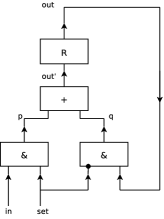
Figure 1. A memory cell

Consider the circuit in Figure 1. The circuit consists of two AND-gates, an OR-gate, a register (depicted by the letter R), and an inverter (depicted by the black dot). The register has output node $\mathsf{reg}$ and input node $\mathsf{reg^{\prime}}$. The value of the output of the register at time $t+1$ is the value of its input at time $t$. The memory cell can be written with the value at node $\mathsf{in}$ by making node $\mathsf{set}$ high.

In STE, circuit specifications are assertions of the form $A\Longrightarrow C$. Here, $A$ is called the antecedent and $C$ the consequent. For example, an STE-assertion for the memory cell is:

$$(\mathsf{in}\mathbf{\>is\>}a)\mathbf{\>\>and\>\>}(\mathsf{set}\mathbf{\>is\>}1)\Longrightarrow\mathrm{\mathbf{N}}(\mathsf{out}\mathbf{\>is\>}a)$$

Here $a$ is a symbolic constant , which can take on the value $0$ or $1$, and $\mathsf{in}$, $\mathsf{set}$ and $\mathsf{out}$ are node names. $\mathrm{\mathbf{N}}$ is the next-time operator. The assertion states that when node $\mathsf{in}$ has value $a$, and node $\mathsf{set}$ has value $1$, then at the next point in time, node $\mathsf{out}$ must have value $a$.

1.2. Generalised Symbolic Trajectory Evaluation

One of the main disadvantages of STE is that it can only deal with properties ranging over a finite number of time-steps. Generalised Symbolic Trajectory Evaluation (GSTE) [gsteIntroduction, gsteCaseStudy, abstractionInAction, gsteNotPublished] is an extension of STE that can deal with properties ranging over unbounded time.

In GSTE, circuit properties are given by assertion graphs. For example, an assertion graph for the memory cell is:

(1)

In the assertion graph, each edge is labelled with a pair $A/C$. As in STE, $A$ is called the antecedent and $C$ is called the consequent. The syntax of $A$ and $C$ is like the syntax of the antecedent and consequent in STE without the next-time operator $\mathrm{\mathbf{N}}$. The $\mathrm{\mathbf{N}}$ operator can not be used because each edge only represents a single time-point. A dot $(\cdot)$ means an empty antecedent or consequent.

The assertion graph above states that if we write value $a$ to the memory cell, and then for arbitrary many time-steps we do not write, the memory cell still contains value $a$.

Each finite path, starting in the initial vertex $\mathsf{init}$ of the graph, represents an STE property. For instance, the finite paths through the assertion graph above represent the following STE properties:

$$\begin{array}[]{lcl}(\mathsf{in}\mathbf{\>is\>}a)\mathbf{\>\>and\>\>}(\mathsf{set}\mathbf{\>is\>}1)&\Longrightarrow&\mathrm{\mathbf{N}}(\mathsf{out}\mathbf{\>is\>}a)\\ (\mathsf{in}\mathbf{\>is\>}a)\mathbf{\>\>and\>\>}(\mathsf{set}\mathbf{\>is\>}1)\mathbf{\>\>and\>\>}\mathrm{\mathbf{N}}(\mathsf{set}\mathbf{\>is\>}0)&\Longrightarrow&\mathrm{\mathbf{N}}\mathrm{\mathbf{N}}(\mathsf{out}\mathbf{\>is\>}a)\\ (\mathsf{in}\mathbf{\>is\>}a)\mathbf{\>\>and\>\>}(\mathsf{set}\mathbf{\>is\>}1)\mathbf{\>\>and\>\>}\mathrm{\mathbf{N}}(\mathsf{set}\mathbf{\>is\>}0)\mathbf{\>\>and\>\>}\mathrm{\mathbf{N}}\mathrm{\mathbf{N}}(\mathsf{set}\mathbf{\>is\>}0)&\Longrightarrow&\mathrm{\mathbf{N}}\mathrm{\mathbf{N}}\mathrm{\mathbf{N}}(\mathsf{out}\mathbf{\>is\>}a)\\ \ldots\end{array}$$

Each of these assertions can be proven by an STE model checker. But, as the set of assertions is infinite, we cannot use plain STE to prove all of them. However, if we use GSTE to prove that the circuit satisfies the above assertion graph, it follows that all STE-assertions represented by the assertion graph hold as well.

Note that in GSTE, just like in STE, the initial values of registers are ignored.

1.3. Earlier work on semantics for GSTE

A semantics for GSTE can be used to predict and understand why certain circuit properties can or cannot be proven by GSTE. In [gsteNotPublished, abstractionInAction] three semantics for GSTE are distinguished: (1) the strong semantics, (2) the normal semantics, and (3) the fair semantics. The semantics have in common that a circuits satisfies an assertion-graph if it satisfies all appropriate paths in the assertion graph. The meaning of appropriate differs over the three semantics, as we explain in the following paragraphs. As in [reasoning], we refer to this class of semantics as the $\forall$-semantics, because these semantics really consider all concrete paths, rather than approximating this quantification by applying abstraction.

In the strong semantics, a circuit satisfies a GSTE assertion graph if-and-only-if the circuit satisfies all STE-assertions corresponding to finite paths in the assertion graph. For instance, as the memory cell satisfies the set of finite assertions above, it also satisfies assertion graph (1).

Consider the following assertion graph:

(2)

Intuitively, we might want the above assertion graph to state that if at some time-point node $\mathsf{out}$ has value $a$, and just before that, node $\mathsf{set}$ was high, then at this time-point node $\mathsf{in}$ should have value $a$. This is an example of a backwards property, that is, a property in which a consequent depends on an antecedent at a later time-point.

The strong semantics cannot deal with such backwards properties. For instance, for the above property, the path starting in vertex $\mathsf{init}$ and ending in vertex $v$ corresponds to the assertion

$$(\mathsf{set}\mathbf{\>is\>}1)\Longrightarrow(\mathsf{in}\mathbf{\>is\>}a)$$

This assertion is, of course, not true for the memory cell. But, any run of the circuit that makes $\mathsf{in}\mathbf{\>is\>}a$ fail, makes $\mathrm{\mathbf{N}}(\mathsf{out}\mathbf{\>is\>}a)$ fail as well. So, intuitively, the assertion is not satisfied because a consequent failed before the antecedent it depended on could fail.

In the normal semantics, a circuit satisfies a GSTE assertion graph if-and-only-if the circuit satisfies the STE-assertions corresponding to all infinite paths in the assertion graph. Therefore, the normal semantics can deal with backwards properties as well. For instance, in assertion graph (2), there is only one infinite path. This path corresponds to the following assertion:

$$(\mathsf{set}\mathbf{\>is\>}1)\mathbf{\>\>and\>\>}\mathrm{\mathbf{N}}(\mathsf{out}\mathbf{\>is\>}a)\Longrightarrow(\mathsf{in}\mathbf{\>is\>}a)$$

As any circuit trace that satisfies the antecedent satisfies the consequent as well, this assertion is satisfied by the circuit. Thus, in the normal semantics, the GSTE assertion graph is satisfied.

Finally, the need for the fair semantics is illustrated by the following example. Consider the assertion graph:

(3)

The assertion graph above states that if at some time-point node $\mathsf{out}$ has value $a$, and before that, for a period of time no values were written to the memory-cell, and before that, $\mathsf{set}$ was high, then at this time-point $\mathsf{in}$ should have value $a$.

In the normal semantics, the memory cell circuit does not satisfy this assertion graph. Consider the infinite path starting in $\mathsf{init}$ and then cycling at the self-loop at $v$ for ever. This path corresponds to the infinite assertion:

$$(\mathsf{set}\mathbf{\>is\>}1)\mathbf{\>\>and\>\>}\mathrm{\mathbf{N}}(\mathsf{set}\mathbf{\>is\>}0)\mathbf{\>\>and\>\>}\mathrm{\mathbf{N}}\mathrm{\mathbf{N}}(\mathsf{set}\mathbf{\>is\>}0)\mathbf{\>\>and\>\>}\ldots\Longrightarrow\mathsf{in}\mathbf{\>is\>}a$$

For a given $a$, this assertion can be falsified by the trace in which value $\neg a$ is written at time 0, and is kept in memory since then.

In the fair semantics for GSTE, this problem is solved by selecting a set of fair edges. The semantics only considers paths that visit every fair edge infinitely often. For instance, if in the above assertion graph the edge from vertex $w$ to itself is made fair, the assertion graph holds in the fair semantics.

1.4. GSTE model checking

In the same papers [gsteNotPublished, abstractionInAction], model checking algorithms for normal, strong and fair GSTE are described. It is proven that the model checking algorithms are sound with respect to their corresponding semantics. However, the algorithms are not complete. The reason is that the $\forall$-semantics do not precisely capture the information loss due to the three-valued abstraction in GSTE.

For example, consider the following circuit

and the following assertion graph

The assertion graph represents the following STE-assertions:

$$\begin{array}[]{lcl}\mathsf{p^{\prime}}\mathbf{\>is\>}1&\Longrightarrow&\mathrm{\mathbf{N}}(\mathsf{out}\mathbf{\>is\>}1)\\ \mathsf{p^{\prime}}\mathbf{\>is\>}0&\Longrightarrow&\mathrm{\mathbf{N}}(\mathsf{out}\mathbf{\>is\>}1)\\ \end{array}$$

Both assertions hold. So, the semantics described above predict that the circuit satisfies the assertion graph.

However, it turns out that the GSTE-algorithm cannot prove the assertion graph! The reason is that GSTE algorithms only compute one three-valued assertion for each edge in the assertion graph. This is in general not enough to take account for all STE assertions corresponding to all paths through the assertion graph, so a certain information loss happens. In this particular case, the state calculated on the edge from $v$ to $w$ gives value $\mathsf{X}$ to node $\mathsf{out}$. This can be explained as follows. The antecedent at the top edge between vertices $\mathsf{init}$ and $v$ requires node $\mathsf{p^{\prime}}$ to have value $1$. The antecedent at the bottom edge requires node $\mathsf{p^{\prime}}$ to have value $0$. Node $\mathsf{p^{\prime}}$ is the input to a register with node $\mathsf{p}$ as output. So, when the edge from $v$ to $w$ is reached via the top edge between $\mathsf{init}$ and $v$ node $\mathsf{p}$ will receive value $1$. When the edge from $v$ to $w$ is reached via the bottom edge between $\mathsf{init}$ and $v$, node $\mathsf{p}$ will receive value $0$. As the value of node $\mathsf{p}$ should comply with both paths, the algorithm chooses value $\mathsf{X}$ for node $\mathsf{p}$, and thus node $\mathsf{out}$ receives value $\mathsf{X}$ as well.

1.5. The problem

The previous example illustrates that the $\forall$-semantics for GSTE discussed previously cannot be used to explain how the three-valued abstraction causes certain properties to be not provable with GSTE. This can lead to situations where seemingly trivial changes to either the circuit or the assertion can suddenly make an assertion not provable anymore.

This is an undesirable situation. We believe that a faithful semantics for GSTE is needed.

A faithful semantics deems a property to be true if-and-only-if the property can be proven by a GSTE-model checker. Without a faithful semantics, a GSTE verification engineer is left to the particular internals of the model checker at hand to understand what can and cannot be proved. Also, a faithful semantics can be used to understand differences between different GSTE model checkers. For example, the GSTE semantics of satGSTE [GSTESAT] is expressed using successive unrollings of the assertion graph as STE assertions. However, the abstraction obtained in that way does not correspond to the abstraction in standard GSTE model checkers. This means that there are assertion graphs for which satGSTE and standard GSTE model checkers give different answers.

To further clarify the importance of a faithful GSTE semantics, we would like to point out that there is a difference between the use of abstraction in (G)STE, and the application of abstraction as a performance enhancer in model checkers for standard temporal logics like LTL and CTL. In the latter case, a model checker might simply give up when it happens to choose an abstraction that is too weak to prove a property, but it is still clear to the verification engineer what the specification means. In (G)STE, what abstraction to use in the model checker is an artefact of the specification, not an artefact of the model checker. So, in (G)STE it is vital to understand what a specification means, separate from a particular model checker, including the abstraction that is specified.

In previous work [steFaithful], we have described a faithful semantics for STE. However, up till now, no faithful semantics for GSTE has been described.

1.6. Our contribution

In this paper, we present a semantics for GSTE that is faithful to the proving power of the GSTE model checking algorithm. Compared to the semantics described in [gsteNotPublished, abstractionInAction], our semantics corresponds to the strong semantics of GSTE. That is, in this paper, we do not consider backwards properties or fairness constraints, which remains future work. One difference with the strong semantics in [gsteNotPublished, abstractionInAction] is that our semantics captures the three-valued abstraction of GSTE precisely, and thus can be used to explain the information loss caused by the three-valued abstraction in GSTE.

Another difference is that our semantics for GSTE follows the same structure as the semantics for STE [steFaithful, ste, indexing]. For instance, where STE deals with sequences to represent abstract circuit behaviour, our GSTE semantics uses sequence graphs. Here, a sequence graph is a mapping from edges in an assertion graph to abstract circuit states. We show that our GSTE semantics is a generalisation of the STE semantics. That is, given a linear assertion graph, the STE-semantics and GSTE-semantics are equivalent. Finally, we state a number of additional properties relating the two semantics.

We believe that our faithful semantics for STE is an important contribution to the research on GSTE for at least two reasons.

First of all, a faithful semantics makes GSTE more accessible to novice users: a faithful semantics enables users to understand the abstraction used in GSTE, without having to understand the details of the model checking algorithm. Additionally, in this paper, we aim at increasing the understanding for GSTE users of subtle cases of information-loss due to abstraction by providing enlightening examples.

Furthermore, a faithful semantics for GSTE can be used as basis for research on new GSTE model checking algorithms and other GSTE tools. To illustrate this, in previous work [roorda], we described a new SAT-based model checking algorithm for STE and proven that it is sound and complete with respect to our faithful semantics for STE presented in [steFaithful]. Without a faithful semantics for STE, we would have been forced to prove the correctness of our algorithm by relating it to other model checking algorithms for STE. This is clearly a more involved and less elegant approach. In fact, we believe that without constructing a faithful semantics for STE first, we would not have obtained the level of understanding of STE needed to develop the new SAT-based model checking algorithm.

In the same way, we expect that the faithful semantics for GSTE presented in this paper will open the door for new research on GSTE model checking algorithms and other GSTE tools.

1.7. Other related work

The following papers are based on the $\forall$-semantics for GSTE.

GSTE as partitioned model checking

In [vardi], the relation between GSTE and classic symbolic model checking is studied. It is explained how GSTE can be seen as a partitioned form of classic symbolic model checking. However, the abstraction of GSTE is not taken into account. Therefore, this paper, focussing on the abstraction in GSTE, is complementary to [vardi].

Using SAT for debugging of GSTE assertion graphs

In [GSTESAT], the tool satGSTE is presented. The tool considers a finite subset of all finite paths in an assertion graphs, for instance, all paths up to a certain length. For each path in this subset, the tool model checks the corresponding STE assertion. The authors explain how the tool can be used to debug and refine GSTE assertion graphs. However, their tool does not follow the same semantics as standard GSTE model checking algorithms. Thus, certain counter examples that would occur in a standard GSTE model checker due to the use of abstraction cannot be found with their algorithm.

Monitor circuits for GSTE assertion graphs

In (conventional, non-symbolic) simulation, a model of a circuit is fed with a large number of inputs. For every input it is checked whether the output is as expected. Typically, a monitor circuit is used to make this check. The monitor circuit observes the system under verification without interfering. During each step of the simulation, it indicates whether the system has obeyed the formal specification thus far.

In [monitor1, monitor2] methods for automatic construction of monitor circuits for GSTE assertion graphs are described. The method in [monitor1] requires the use of a symbolic simulator if the assertion graph contains symbolic constants. In [monitor2] it is explained how, for the class of so-called simulation friendly assertion graphs, the method of [monitor1] can be extended to deal with symbolic constants even in conventional non-symbolic simulation.

The papers explain how monitor circuits can be used to make a bridge between GSTE model checking and conventional simulation. For instance, monitor circuits can be used to quickly debug and refine GSTE specifications before trying to use more labour intensive GSTE model checking.

Reasoning about GSTE assertion graphs

Using the construction of monitor circuits for GSTE assertion graphs, [reasoning] describes two algorithms that can be used in compositional verification using GSTE. The first algorithm decides whether one assertion graph implies another. The second algorithm can be used to model check an assertion graph under the assumption that another assertion graph is true.

1.7.1. Relation to this paper

Each of the papers above is based on the $\forall$-semantics for GSTE. As explained above, the $\forall$-semantics are not faithful to the proving power of the GSTE model checking algorithms. So, it can occur that a tool described in the papers deems a GSTE assertion to be true, while the GSTE model checking algorithm cannot prove it.

For instance, the monitor circuits described above cannot be used to debug and refine assertions graphs that are true in the $\forall$-semantics but yield a spurious counter-example when trying to prove them with a GSTE model checker. The satGSTE tool is limited in the same way. We elaborate further on this in the future work section of this paper.

1.8. Structure of this paper

In the next section, we revisit the semantics of STE assertions. Then, in Section 3, we present our semantics of GSTE assertion graphs. In Section 4, we compare the STE semantics with the GSTE semantics by giving a number of properties describing their relation. In Section 5, we describe the GSTE model checking algorithm and show that it is sound and complete with respect to our semantics. Finally, in Section 6, we conclude and give suggestions for future work.

2. STE Preliminaries

A semantics for STE was first described by Seger and Bryant [ste]. Later, a simplified and easier to understand semantics was given by Melham and Jones [indexing]. Both of these semantics are expressed in terms of a next state function, expressing the relationship between two consecutive states in the circuit. Unfortunately, neither of these semantics matches the proving power of currently available STE model checkers. The problem is that they cannot deal with combinational properties (properties ranging over one single point in time). All such properties are deemed to be false by the semantics. Therefore standard next state semantics does not seem to be a good starting point for finding a faithful semantics for GSTE.

In previous work [steFaithful], we have described an alternative semantics for STE that actually is faithful to the proving power of STE model checkers. The semantics is called the closure semantics. Informally, the closure semantics only differs from the traditional STE semantics for combinational properties.

A main ingredient of the closure semantics for STE is the concept of a closure function. The idea is that a closure function takes as input a state of the circuit, and calculates all information about the circuit state at the same point in time that can be derived by propagating the information in the input state in a forwards fashion. In the next section, we give an alternative semantics for GSTE also based on closure functions.

In this section we briefly describe the closure semantics for STE. For more examples and a discussion on the differences with the semantics given in [ste, indexing], we refer the reader to [steFaithful].

Readers familiar with [steFaithful] can skip most of this section; compared to [steFaithful] we slightly changed notation in the definition of the closure function on sequences, and we introduced an extra variant of a closure semantics called the simple semantics. Furthermore, we adapted the terminology to GSTE: we call the variables in STE-assertions symbolic constants to indicate that they keep a constant value over time. Finally, we use finite sequences to represent circuit behaviour, as opposed to the standard use of infinite sequences. Notice that this is a very superficial change on the notational level; it does not change the semantics itself. The reason for making the change is that it enables us to considerably simplify the proof of Proposition LABEL:prop:compare on page LABEL:prop:compare.

Figure 2. The STE lattice

2.1. Values and Circuits States

Values  In STE, we can abstract away from specific Boolean values of a node, by using the value $\mathsf{X}$, which stands for unknown. The value $\mathsf{T}$ stands for over constrained. A node takes on the value $\mathsf{T}$ when is required to have both value $0$ and value $1$.

On this set an information-ordering $\leq$ is introduced, see Figure 2. The unknown value $\mathsf{X}$ contains the least information, so $\mathsf{X}\leq 0$ and $\mathsf{X}\leq 1$, while $0$ and $1$ are incomparable. The over-constrained value contains the most information, so $0\leq\mathsf{T}$ and $1\leq\mathsf{T}$. If $v\leq w$ it is said that $v$ is weaker than $w$.

$$\begin{array}[]{ccccccccc}\begin{array}[]{c|c}v&\neg v\\ \hline\cr 0&1\\ 1&0\\ \mathsf{X}&\mathsf{X}\\ \mathsf{T}&\mathsf{T}\\ \end{array}&&\begin{array}[]{c|cccc}\>\&&0&1&\mathsf{X}&\mathsf{T}\\ \hline\cr 0&0&0&0&\mathsf{T}\\ 1&0&1&\mathsf{X}&\mathsf{T}\\ \mathsf{X}&0&\mathsf{X}&\mathsf{X}&\mathsf{T}\\ \mathsf{T}&\mathsf{T}&\mathsf{T}&\mathsf{T}&\mathsf{T}\\ \end{array}&&\begin{array}[]{c|cccc}\>\mathbf{+}&0&1&\mathsf{X}&\mathsf{T}\\ \hline\cr 0&0&1&\mathsf{X}&\mathsf{T}\\ 1&1&1&1&\mathsf{T}\\ \mathsf{X}&\mathsf{X}&1&\mathsf{X}&\mathsf{T}\\ \mathsf{T}&\mathsf{T}&\mathsf{T}&\mathsf{T}&\mathsf{T}\\ \end{array}&&\begin{array}[]{c|cccc}\sqcup&0&1&\mathsf{X}&\mathsf{T}\\ \hline\cr 0&0&\mathsf{T}&0&\mathsf{T}\\ 1&\mathsf{T}&1&1&\mathsf{T}\\ \mathsf{X}&0&1&\mathsf{X}&\mathsf{T}\\ \mathsf{T}&\mathsf{T}&\mathsf{T}&\mathsf{T}&\mathsf{T}\\ \end{array}&&\begin{array}[]{c|cccc}\sqcap&0&1&\mathsf{X}&\mathsf{T}\\ \hline\cr 0&0&\mathsf{X}&\mathsf{X}&0\\ 1&\mathsf{X}&1&\mathsf{X}&1\\ \mathsf{X}&\mathsf{X}&\mathsf{X}&\mathsf{X}&\mathsf{X}\\ \mathsf{T}&0&1&\mathsf{X}&\mathsf{T}\\ \end{array}\end{array}$$

Figure 3. Four-valued extensions of the logical operators, least upper bound and greatest lower bound operators.

The set $V$ together with the ordering $\leq$ forms a lattice. The least upper bound operator is written $\sqcup$, the greatest lower bound operator is written $\sqcap$, see Figure 3.

The logical operators for conjunction, written $\>\&\>$, disjunction, written $\>\mathbf{+}\>$, and negation, written $\neg$, are extended to the four-valued domain as in Figure 3.

States  A circuit state, written $s:\mathbf{State}$, is a function from the set of nodes of a circuit to the values $\{0,1,\mathsf{X},\mathsf{T}\}$.

2.2. Closure functions

In our semantics for STE, closure functions are used as circuit models. The idea is that a closure function, written $F:\mathbf{State}\rightarrow\mathbf{State}$ takes as input a state of the circuit, and calculates all information about the circuit state at the same point in time that can be derived by propagating the information in the input state in a forwards fashion.

The closure function for a circuit consisting of a single AND-gate with inputs $\mathsf{p}$ and $\mathsf{q}$, and output $\mathsf{r}$ is given by the table below. Here, $s$ is a state and $n$ is a node.

$$\begin{array}[]{l|l}n&F(s)(n)\\ \hline\cr\mathsf{p}&s(\mathsf{p})\\ \mathsf{q}&s(\mathsf{q})\\ \mathsf{r}&(s(\mathsf{p})\>\&\>s(\mathsf{q}))\sqcup s(\mathsf{r})\\ \end{array}$$

The least upper bound operator in the expression for $F(s)(\mathsf{r})$ combines the value of $\mathsf{r}$ in the given state $s$, and the value for $\mathsf{r}$ that can be derived from the values of $\mathsf{p}$ and $\mathsf{q}$, being $s(\mathsf{p})\>\&\>s(\mathsf{q})$.

A state $s:\{\mathsf{p},\mathsf{q},\mathsf{r}\}\rightarrow\mathbb{V}$ can be written as a vector $s(\mathsf{p}),s(\mathsf{q}),s(\mathsf{r})$. For example, the state that assigns the value 1 to nodes $\mathsf{p}$ and $\mathsf{q}$ and the value $\mathsf{X}$ to node $\mathsf{r}$ is written as $11\mathsf{X}$. Applying the closure function to the state $11\mathsf{X}$ yields $111$. The reason is that when both inputs to the AND-gate have value $1$, then by forwards propagation of information, also the output has value $1$. Applying the closure function to state $1\mathsf{X}\mathsf{X}$ yields $1\mathsf{X}\mathsf{X}$. The reason is that the output of the AND-gate is unknown when one input has value $1$ and the other value $\mathsf{X}$. The forwards nature of simulation becomes clear when the closure function is applied to state $\mathsf{X}\mathsf{X}1$, resulting in $\mathsf{X}\mathsf{X}1$. Although the inputs to the AND-gate must have value $1$ when the output of the gate has value $1$, this cannot be derived by forwards propagation.

A final example shows how the over-constrained value $\mathsf{T}$ can arise. Applying the closure function to state $0\mathsf{X}1$ yields $0\mathsf{X}\mathsf{T}$. The reason is that the input state gives node $\mathsf{r}$ value $1$ and node $\mathsf{p}$ value $0$. From $\mathsf{p}$ having value $0$ it can be derived by forwards propagation that $\mathsf{r}$ has value $0$, therefore $\mathsf{r}$ receives the over-constrained value $\mathsf{T}$. ∎ A closure function is a function $F:\mathbf{State}\rightarrow\mathbf{State}$ satisfying the following three conditions:

1. $F$ is monotonic, that is, for all states $s_{1},s_{2}$: $s_{1}\leq s_{2}$ implies $F(s_{1})\leq F(s_{2})$. This means that a more specified input state cannot lead to a less specified result. The reason is that given a more specified input state, more information about the state of the circuit can be derived.

2. $F$ is idempotent, that is, for every state $s$: $F(F(s))=F(s)$. This means that repeated application of the closure function has the same result as applying the function once. The reason is that the closure function should derive all information about the circuit state in one go.

3. $F$ is extensive, that is, for every state $s$: $s\leq F(s)$. This means that the application of a closure function to a circuit state should yield a state at least as specified as the input state. The reason is that the closure function is required not to lose any information.

Netlists  Here, a netlist is an acyclic list of definitions describing the relations between the values of the nodes. Inverters are not modelled explicitly in our netlists, instead they occur implicitly for each mention of the negation operator $\neg{}$ on the inputs of the gates. Registers are not mentioned explicitly in the netlist either. Instead, for a register with output node $n$ in the circuit, the input of the register is node $n^{\prime}$ which is mentioned in the netlist. For simplicity, we only allow AND-gates and OR-gates in netlists. It is, however, straightforward to extend this notion of netlists to include more operations.

Induced Closure Function  Given the netlist of a circuit $c$, the induced closure function for the circuit, written $F_{c}$, can easily be constructed by interpreting each definition in the netlist as a four-valued gate (see Figure 3). Each

Given a state $s$, a circuit $c$, and a circuit node $n$, we calculate $F_{c}(s)(n)$ as follows:

1. If $n$ is a circuit input or the output of a register, then we define $F_{c}(s)(n)=s(n)$.

2. If $n$ is the output of an AND-gate with input nodes $p$ and $q$, then we define

   $$F_{c}(s)(n)=(F_{c}(s)(p)\>\&\>F_{c}(s)(q))\sqcup s(n).$$

3. If $n$ is the output of an OR-gate with input nodes $p$ and $q$, then we define

   $$F_{c}(s)(n)=(F_{c}(s)(p)\>\mathbf{+}\>F_{c}(s)(q))\sqcup s(n).$$

4. If $n$ is the output of an inverter with input node $p$, then we define

   $$F_{c}(s)(n)=\neg F_{c}(s)(p)\sqcup s(n).$$

This definition is well-defined because netlists are acyclic by definition.

Proposition 1.

The induced closure function for a circuit is by construction monotonic, idempotent and extensive.

Proof 2.1.

The closure function $F_{c}$ is a composition of the monotonic functions of four-valued negation, four-valued conjunction and least upper bound, therefore it is monotonic itself.

As netlists are acyclic by definition, we can prove properties by induction over the definition of a node. We prove idempotency by proving $F_{c}(F_{c}(s))(n)=F_{c}(s)(n)$ by induction on the definition of $n$. Assume $n$ is in the set of input- and state-holding nodes $\mathcal{I}\cup\mathcal{S}$, then $F_{c}(F_{c}(s))(n)=F_{c}(s)(n)$ by definition. If $n$ is defined by $n=p\;\mbox{\sc and}\;q$, then:

$$\begin{array}[]{lll}&F_{c}(F_{c}(s))(n)\\ =&(F_{c}(F_{c}(s))(p)\>\&\>F_{c}(F_{c}(s))(q))\>\sqcup\>F_{c}(s)(n)&($definition$)\\ =&(F_{c}(s)(p)\>\&\>F_{c}(s)(q))\>\sqcup\>F_{c}(s)(n)&($ind. hyp.$)\\ =&(F_{c}(s)(p)\>\&\>F_{c}(s)(q))\>\sqcup\>(F_{c}(s)(p)\>\&\>F_{c}(s)(q))\>\sqcup\>s(n)&($definition$)\\ =&(F_{c}(s)(p)\>\&\>F_{c}(s)(q))\>\sqcup\>s(n)&($property $\sqcup)\\ =&F_{c}(s)(n)&($definition$)\end{array}$$

A similar argument holds when $n$ is defined by a different gate definition.

The extensivity of $F_{c}$ follows directly from its definition: If $n$ is an input or state holding node then $F_{c}(s)(n)=s(n)$, otherwise $F(c)(n)$ is defined as the least upper bound of $s(n)$ and another expression, so $s(n)\leq F_{c}(s)(n)$. ∎

2.3. A closure function for sequences

Sequences  A sequence of depth $d$, written $\sigma:\{0,1,\ldots,d\}\rightarrow\mathbf{State}$, is a function from a point in time to a circuit state, describing the behaviour of a circuit over time. The set of all sequences is written $\mathbf{Seq}$. A three-valued sequence is a sequence that does not assign the value $\mathsf{T}$ to any node at any time.

The order $\leq$ and the operators $\sqcup$ and $\sqcap$ are extended to sequences in a point-wise fashion. That is, the order $\leq$ on sequences is defined by $\sigma_{1}\leq\sigma_{2}$ iff for all $n$, $\sigma_{1}(n)\leq\sigma_{2}(n)$. Furthermore, $(\sigma_{1}\sqcup\sigma_{2})(n)=(\sigma_{1}(n)\sqcup\sigma_{2}(n))$, and $(\sigma_{1}\sqcap\sigma_{2})(n)=(\sigma_{1}(n)\sqcap\sigma_{2}(n))$.

Closure for sequences  In STE, a circuit is simulated over multiple time steps. During simulation, information is propagated forwards through the circuit and through time, from each time step $t$ to time step $t+1$. Note that the initial values of registers are ignored.

To model this forwards propagation of information through time, a closure function for sequences, notation $F^{\rightarrow}:\mathbf{Seq}\rightarrow\mathbf{Seq}$, is used. Given a sequence, the closure function for sequences calculates all information that can be derived from that sequence by forwards propagation. The closure function for sequences preserves the depth of the given sequence.

Recall that for every register with output $n$, the input to the register is node $n^{\prime}$. Therefore, the value of node $n^{\prime}$ at time $t$ is propagated to node $n$ at time $t+1$ in the forwards closure for sequences.

Given a circuit state $s$, the function $\mathrm{next}$ calculates the information that is propagated by the registers, and is defined by:

$$\mathrm{next}(s)(n)=\left\{\begin{array}[]{ll}s(n^{\prime}),&n\in\mathcal{S}\\ \mathsf{X},&\text{otherwise}\end{array}\right.$$

The closure function for sequences $F^{\rightarrow}$ is defined in terms of a closure function $F$. Given a closure function $F$ for a circuit with a set of outputs of registers $\mathcal{S}$, the closure function for sequences, written $F^{\rightarrow}:\mathbf{Seq}\rightarrow\mathbf{Seq}$, is inductively defined by:

$$\begin{array}[]{lcllr}F^{\rightarrow}(\sigma)(0)&=&F(\sigma(0))&\\ F^{\rightarrow}(\sigma)(t+1)&=&F(\>\sigma(t+1)\>\sqcup\>\mathrm{next}(F^{\rightarrow}(\sigma)(t))\>)&&(0\leq t\leq d-1)\\ \end{array}$$

Proposition 2.

The function $F^{\rightarrow}$ inherits the properties of being monotonic, idempotent and extensive from $F$.