Abstract

The cat-eyes steady state solution in the framework of hydrodynamics describing an infinite row of identical vortices is extended to the magnetohydrodynamic (MHD) equilibrium equation with incompressible flow of arbitrary direction. The extended solution covers a variety of equilibria including one- and two-dimensional generalized force-free and Harris-sheet configurations which are preferable from those usually employed as initial states in reconnection studies. Although the vortex shape is not affected by the magnetic field, the flow in conjunction with the equilibrium nonlinearity has a strong impact on isobaric surfaces by forming pressure islands located within the cat-eyes vortices. More importantly, a magnetic-field-aligned flow of experimental fusion relevance and the flow shear have significant stabilizing effects in the region of pressure islands. The stable region is enhanced by an external axial (“toroidal”) magnetic field.

Sheared flows influence the equilibrium and stability properties of magnetically confined plasmas and result in transitions to improved modes either in the edge region (low-to-high-mode transition) or in the central region (internal transport barriers) of fusion devices. As concerns equilibrium, the convective velocity term in the momentum equation makes the isobaric surfaces to deviate from magnetic surfaces, unlike the case of quasistatic steady states [1], thus potentially affecting stability. For symmetric two dimensional equilibria, this effect has been examined on the basis of analytic solutions to linearized forms of generalized Grad-Shafranov equations, e.g. Ref. [2]. For flows of fusion concern, i.e. for Alfvén Mach numbers of the order of 0.01, this deviation is small and consequently isobaric and magnetic surfaces have the same topology.

Aim of the present study is to examine the impact of flow in conjunction with nonlinearity to certain equilibrium and stability properties in relation to the departure of the isobaric from magnetic surfaces. Motivation was a solution of a nonlinear form of the hydrodynamic equation describing the steady motion of an inviscid incompressible fluid in two dimensional plane geometry, known as “cat eyes”, which represents an infinite row of identical vortices ([3, 4]; see also Fig. 1). This solution is extended here to the MHD equilibrium equation with incompressible flow. Then, the stability of the extended solution is examined by means of a recent sufficient condition [5]. The major conclusion is that owing to the nonlinearity of the equilibrium, the flow and flow shear affect drastically the pressure surfaces and have significant stabilizing effects in the region of modified pressure.

The MHD equilibrium equations with incompressible flow for translationally symmetric plasmas are reviewed in Sec. II. In Sec. III a solution of the pertinent generalized Grad-Shafranov equation describing a whole set of equilibria is constructed as an extension of the cat-eyes solution. Then for parallel flows and constant density the stability of the solution obtained is studied in Sec. IV. Sec. V recapitulates the study and summarizes the conclusions.

The MHD equilibrium states of a translationally symmetric magnetized plasma with incompressible flows satisfy the generalized Grad-Shafranov equation [6],

$$(1-M^{2})\nabla^{2}\psi-\frac{1}{2}(M^{2})^{\prime}|\nabla\psi|^{2}+\left(Ps+\frac{B_{z}^{2}}{2}\right)^{\prime}=0$$ (1)

and the Bernoulli relation for the pressure

$$P=P_{s}(\psi)-\frac{1}{2}M^{2}\left|\nabla\psi\right|^{2}.$$ (2)

Here, the function $\psi(x,y)$ labels the magnetic surfaces with $(x,y,z)$ Cartesian coordinates so that $z$ corresponds to the axis of symmetry and ($x,y$) are associated with the poloidal plane; $M(\psi)$ is the Mach function of the poloidal velocity with respect to the poloidal-magnetic-field Alfvén velocity; $B_{z}$ is the axial magnetic field; for vanishing flow the surface function $P_{s}(\psi)$ coincides with the pressure; the prime denotes a derivative with respect to $\psi$. The surface quantities $M(\psi)$, $B_{z}(\psi)$ and $P_{s}(\psi)$ are free functions for each choice of which (1) is fully determined and can be solved whence the boundary condition for $\psi$ is given. Also, to completely determine the equilibrium, a couple of additional surface functions are needed, i.e, the density, $\varrho(\psi)$, and the electrostatic potential, $\Phi(\psi)$. Details including derivation of (1) and (2) can be found in Refs. [6, 7].

Eq. (1) can be simplified by the transformation [8, 9]

$$u(\psi)=\int_{0}^{\psi}\left[1-M^{2}(g)\right]^{1/2}dg,$$ (3)

which reduces (1) to

$$\nabla^{2}u+\frac{d}{du}\left(P_{s}+\frac{B_{z}^{2}}{2}\right)=0.$$ (4)

Also, (2) is put in the form

$$P=P_{s}(u)-\frac{M^{2}}{2(1-M^{2})}\left|\mbox{\boldmath${\nabla}$}u\right|^{2}.$$ (5)

Note that (4) free of a quadratic term as $|{\bf\nabla}u|^{2}$ is identical in form with the quasistatic MHD equilibrium equation as well as to the equation governing the steady motion of an inviscid incompressible fluid in the framework of hydrodynamics. Transformation (3) does not affect the magnetic surfaces, it just relabels them. Also, once a solution of (4) is found, the equilibrium can be completely constructed in the $u$-space; in particular, the magnetic field, current density, velocity, and electric field can be determined by the relations:

$${\mathbf{B}} = B_{z}{\mathbf{e}}_{z}+\left(1-M^{2}\right)^{-1/2}{\mathbf{e}}_{z}\mbox{\boldmath$\times$}\mbox{\boldmath${\nabla}$}u$$ (6)

$${\mathbf{j}} = \left[\left(1-M^{2}\right)^{-1/2}\mbox{\boldmath${\nabla}$}^{2}u+\frac{1}{2}\frac{{d}M^{2}}{{d}u}\left(1-M^{2}\right)^{-3/2}\left|\mbox{\boldmath${\nabla}$}u\right|^{2}\right]{\mathbf{e}}_{z}$$

$$-\frac{{d}B_{z}}{{d}u}{\mathbf{e}}_{z}\mbox{\boldmath$\times$}\mbox{\boldmath${\nabla}$}u$$

$${\mathbf{v}} = \frac{M}{\sqrt{\varrho}}{\mathbf{B}}-\left(1-M^{2}\right)^{-1/2}\frac{{d}\Phi}{{d}u}{\mathbf{e}}_{z}$$ (8)

$${\mathbf{E}} = -\frac{{d}\Phi}{{d}u}\mbox{\boldmath${\nabla}$}u.$$ (9)

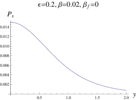
Figure 2: Profile of the quasistatic pressure function $P_{s}$ [Eq. (14)] along the $y-$axis.

Analytic solutions to linearized forms of (4) have been constructed for quasistatic [10, 11] and stationary equilibria [7]. As already mentioned in Sec. I, for flows of experimental fusion relevance ($|M|\approx 0.01$) the departure of the isobaric from magnetic surfaces is small (see for example Fig. 2 of Ref. [2]), so that the topology of these two families of surfaces is identical.

II.  Magnetohydrodynamic “cat eyes” with flow

The present section aims at extending the hydrodynamic cat-eyes solution to (4) and examine certain equilibrium characteristics in connection with the impact of the flow together with nonlinearity. For convenience we introduce dimensional quantities: $\tilde{x}=x/L$, $\tilde{y}=y/L$, $\tilde{u}=u/(B_{z0}L)$, $\tilde{\varrho}=\varrho/\varrho_{0}$, $\tilde{P}=P/B_{z0}^{2}$, $\tilde{{\mathbf{B}}}={\mathbf{B}}/B_{z0}$, $\tilde{{\mathbf{j}}}={\mathbf{j}}/(B_{z0}/L)$, $\tilde{{\mathbf{v}}}={\mathbf{v}}/v_{A0}$, where $v_{A0}=B_{z0}/\sqrt{\varrho_{0}}$ , and $\tilde{{\mathbf{E}}}={\mathbf{E}}/(B_{z0}v_{A0})$; here, $L$, $B_{z0}$, and $\varrho_{0}$ are reference quantities to be defined later. Eqs. (4) and (5) hold in identical forms for the tilted quantities and will be further employed as dimensionless by dropping for simplicity the tilde. To construct a cat-eyes solution we make the ansatz

$$\frac{{d}(P_{s}+B_{z}^{2}/2)}{{d}u}=(\epsilon^{2}-1)\exp(-2u),$$ (10)

by which (4) reduces to the following form of Liouville’ s equation:

$$\nabla^{2}u=(1-\epsilon^{2})\exp(-2u).$$ (11)

Eq. (11) admits the solution

$$u=\ln\left[\cosh(y)-\epsilon\cos(x)\right],$$ (12)

the characteristic lines of which are shown in Fig. 1. The parameter $\epsilon$ determines the vortex size; for $\epsilon=1$ the solution represents an infinite row of point vortices and for $\epsilon=0$ it becomes one-dimensional: $u=\ln\cosh y$. It is noted here that though (12) is singular in the limit of $y\rightarrow\infty$, all the local equilibrium quantities are everywhere regular. Eq. (10) can be solved for $P_{s}(u)+B_{z}^{2}/2$ to yield

$$P_{s}+\frac{B_{z}^{2}}{2}=\frac{1-\epsilon^{2}}{2}\exp{(-2u)}+c_{0}=\frac{1-\epsilon^{2}}{2\left(\cosh y-\epsilon\cos x\right)^{2}}+c_{0},$$ (13)

where $c_{0}$ is a constant. The equilibria described by (12) and (13) have the following characteristics:

1. The vortices are by construction of solution (12) identical to the respective hydrodynamic vortices, viz., the magnetic field does not affect the vortex shape.

2. Since magnetic field and current density lie on the velocity or magnetic surfaces, the vortices can be regarded as magnetic islands with plasma flow. Quasistatic MHD and hydrodynamic cat eyes can be recovered as particular cases. Also, it may be noted that for flows non parallel to the magnetic field, the electric field is perpendicular to the magnetic surfaces [Eq. (9)].

3. In fact, (12) and (13) hold for a rather large set of equilibria because the functions $\rho(u)$, $\Phi(u)$, $M(u)$ and one out of $B_{z}(u)$ and $P_{s}(u)$ remain free.

We will further consider a subset of steady sates by assigning the free functions $P_{s}$, $B_{z}$ and $M$ as

$$P_{s}(u)=\beta\frac{1-\epsilon^{2}}{2}\exp{(-2u)}+\frac{\beta_{f}}{2},$$ (14)

$$B_{z}^{2}(u)=(1-\beta)(1-\epsilon^{2})\exp{(-2u)}+B_{z0}^{2},$$ (15)

$$M=M_{0}\exp(-2nu)=M_{0}\left(\cosh y-\epsilon\cos x\right)^{-2n},\ \ n>0.$$ (16)

Choice (16) yields a peaked $M^{2}$-profile along $y$ with $|M_{0}|$ being the maximum absolute value at $x=y=0$. The profile becomes steeper as $n$ takes larger positive values, thus increasing the shear of $M$ in relation to the velocity shear. Henceforth, profiles will refer to the $y$-axis. The parameter $B_{z0}$ represents the external axial magnetic field,

$$\beta=\frac{P_{s}(\epsilon=y=0)}{B_{z0}^{2}/2}$$

and $\beta_{f}=P_{s0}/(B_{z0}^{2}/2)$, where $P_{s0}=\mbox{const}$. Note that $\beta$ has been introduced in (14) and (15) in such a way that (13) is automatically satisfied. The other parameter $\beta_{f}$ in (14) yields force-free quasistatic equilibria when $\beta=0$. For $\beta\neq 0$, we set $\beta_{f}=0$ in order that $P_{s}$ vanishes for $y\rightarrow\infty$; thus, only one of the parameters $\beta$ and $\beta_{f}$ is finite in connection with peaked and flat $P_{s}$-profiles, respectively. For flat $P_{s}$-profiles, to guarantee positiveness of the pressure for $\beta_{f}\geq 0$, Eq. (5) is modified to:

$$P=\frac{\beta_{f}}{2}-\frac{M^{2}}{2(1-M^{2})}\left|\mbox{\boldmath${\nabla}$}u\right|^{2}+\frac{M_{0}^{2}}{2(1-M_{0}^{2})}.$$ (17)

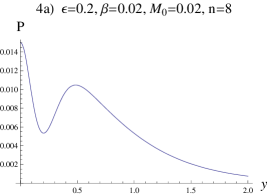
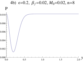
Figure 4: Pressure profiles along the $y$-axis respective to the pressure-island configurations 3a and 3b. For vanishing flow the profiles 4a and 4b become peaked and flat, respectively.

The parameters $M_{0}$, and $n$ are free together with $L$, $\varrho_{0}$, $\epsilon$, $B_{z0}$, and $\beta$ or $\beta_{f}$. It is recalled that dimensionless quantities are employed and therefore $B_{z0}=1$. Also, the reference quantities $L$ and $\varrho_{0}$ not appearing explicitly in the equations can arbitrarily be defined as the vortex length (along the $x$-axis) and the density at $x=y=0$. Because of the many free parameters, there is a variety of steady states including extensions of equilibria employed as initial states in reconnection studies (see for example Ref. [12]). An example concerns the one-dimensional, force free quasistatic equilibrium recovered for $\beta=\epsilon=0$. In the presence of flow and $\epsilon\neq 0$ this equilibrium becomes two-dimensional with hollow pressure profile (Eq. (17); see also Fig. 4b). Also, in this case both current density and velocity have all three components finite. Another example for $\beta=1$ is an equilibrium with $B_{z}=B_{z0}$, axial current density and three-component velocity. For vanishing flow and $\epsilon=0$ this reduces to the Harris sheet equilibrium [13].

We have examined the pressure by Mathematica 6 within broad regions of the free parameters, i.e., $0\leq\epsilon\leq 1$, $0\leq\beta\leq 0.9$, $0\leq M_{0}\leq 0.9$ and $0\leq n\leq 15$. Note that, because of the flow term in (5) the pressure for certain parametric values can become negative. Thus, particular care has been taken in getting everywhere physically acceptable pressure. For two dimensional equilibria, it turns out that the flow has strong impact on the isobaric surfaces by creating “pressure islands” within the cat eyes. This is shown in Fig. 3. Also $P$-profiles are presented in Fig. 4. As can be seen in Fig. 3 pressure islands appear even for parametric values of experimental fusion concern ($\beta=0.02$, $M_{0}=0.02$). Since for linear equilibria the flow impact on the pressure is weak, it is the nonlinearity here which should play an important role. Also, as will be discussed in Sec. III, the formation of pressure islands may be related to appreciable stabilizing effects of the flow.

II.  Stabilizing effects of the flow

The stability of the equilibria described by (12) and (14)-(16) is now examined by applying a recent sufficient condition [5]. This condition states that a general steady state of a plasma of constant density and incompressible flow parallel to ${\mathbf{B}}$ is linearly stable to small three-dimensional perturbations if the flow is sub-Alfvénic ($M^{2}<1$) and $A\geq 0$, where $A$ is given by Eq. (20) of Ref. [5]. Consequently, we restrict the study to parallel flows and set $\varrho=1$. First it is noted that on the basis of Mercier expansions it turns out that the condition is never satisfied in the vicinity of the magnetic axis ($A<0$) [14]. This holds for generic two-dimensional equilibria irrespective of the geometry. Also, for the pressure (17), the quantity $A$ is independent of $\beta_{f}$, as may be expected on physical grounds, because $A$ contains $dP_{s}/du$ and not $P_{s}$ itself. In the $u$-space for translationally symmetric equilibria, $A$ assumes the form

$$A = -g^{2}\left\{\left({\mathbf{j}}\mbox{\boldmath$\times$}\mbox{\boldmath${\nabla}$}u\right)\cdot\left({\mathbf{B}}\cdot\mbox{\boldmath${\nabla}$}\right)\mbox{\boldmath${\nabla}$}u+\frac{1}{2}\frac{dM^{2}}{du}\left(1-M^{2}\right)^{-1}\left|\mbox{\boldmath${\nabla}$}u\right|^{2}\right.$$ (18)

$$\left.\left[\left(1-M^{2}\right)^{-1/2}\mbox{\boldmath${\nabla}$}u\cdot\frac{\mbox{\boldmath${\nabla}$}B^{2}}{2}+g(1-M^{2})^{-1}\left|\mbox{\boldmath${\nabla}$}u\right|^{2}\right]\right\},$$

where

$$g=(1-M^{2})^{-1/2}\left(\frac{dP_{s}}{du}-\frac{dM^{2}}{du}\frac{B^{2}}{2}\right),$$ (19)

and ${\mathbf{B}}$ and ${\mathbf{j}}$ as given by (6) and (7). To calculate $A$ analytically for the equilibria under consideration we developed a code in Mathematica 6. The expressions obtained for both peaked and flat $P_{s}$-profiles being lengthy are not given explicitly here except for the case of quasistatic equilibria [Eq. (20) below]. The calculations led to the following conclusions.

1. For quasistatic equilibria ($M_{0}=0$) the quantity $A$ assumes the concise form

   $$A=\frac{\epsilon(1-\epsilon^{2})\left[\epsilon\cosh(y)\sin(x)^{2}+\cos(x)\sinh(y)^{2}\right]}{\left[\epsilon\cos(x)-\cosh(y)\right]^{5}}.$$ (20)

   Note that $A$ becomes independent of $\beta$ and $B_{z0}$. The condition is nowhere satisfied in the island region except for one dimensional configurations ($\epsilon=0$), point vortices ($\epsilon=1$), the magnetic axes, the $x$-points and for $y\rightarrow\infty$ for which $A=0$. A profile of $A$ is given in Fig. 5.

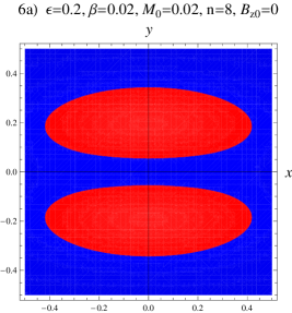
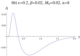
Figure 6: Stabilization effect of flow: In the presence of flow the red colored stable regions appear in the diagram 6a where $A\geq 0$. The respective stable window can be seen in the profile of $A$ in 6b.

2. The flow results in the formation of a stable region close to the magnetic axis in the location of pressure islands. An example shown the sign of $A$ on the poloidal plane is presented in Fig. 6a. The red colored regions are stable ($A\geq 0$), while in the blue colored region it holds $A<0$. The whole area of Fig. 6a becomes blue colored when $M_{0}=0$.

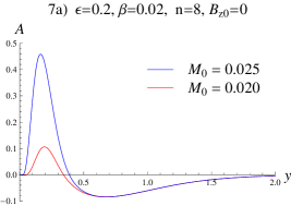
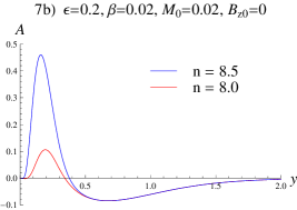
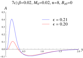
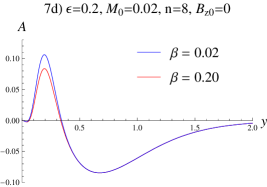
Figure 7: Impact of the flow (7a), flow shear (7b), cat-eyes size (7c) and thermal pressure (7d) in connection with a variation of the parameters $M_{0}$, $n$ and $\epsilon$, and $\beta$, respectively, on the flow caused stable window associated with $A\geq 0$ for the equilibrium of Fig. 3a.

3. The stable region broadens when the parameters $M_{0}$, $n$ and $\epsilon$ take larger values as can be seen in Figs. 7a, 7b and 7c, respectively. Note the sensitiveness of $A$ in the region of the stable window to the small variation of these parameters possibly related to the nonlinearity; in particular, $\epsilon$ appears in the argument of the cat-eyes solution (12). These results hold for both peaked- and flat-$P_{s}$ equilibrium profiles. Unlikely, the stable region is rather insensitive to the variation of $\beta$. An example is given in Fig. 7d, where the stable window persists (just getting slightly smaller) when $\beta$ is increased by an order of magnitude (from 0.02 to 0.2). Also, for point vortices ($\epsilon=1$) $A$ becomes independent of $\beta$ irrespective of the value of $M_{0}$.

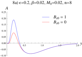
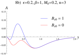
Figure 8: Combined stabilization effect of flow and $B_{z0}$: The curve 8a indicates a stabilizing synergism of $B_{z0}$ and flow for the equilibrium of Fig. 3a. A stronger synergism of this kind is shown in Fig. 8b pertaining to a two-dimensional Harris-type equilibrium.

4. Although for $M_{0}=0$ the vacuum magnetic field $B_{z0}$ has no impact on $A$ [Eq. (20)], in combination with the flow, $B_{z0}$ can enhance the stable region. An example of this synergetic effect is shown in Fig. 8a. Another example of such a strong synergism can be seen in Fig. 8b for a two-dimensional Harris-type equilibrium ($\beta=1$, $\epsilon\neq 0$). In this case, while the flow itself can not make $A$ positive, together with $B_{z0}$ it results in the formation of the stable window.

V.  Summary and Conclusions

We have extended the “cat-eyes” solution of the hydrodynamic equilibrium equation to cover MHD magnetically confined plasmas with incompressible flow. The extension was accomplished smoothly because the pertinent generalized Grad-Shafranov equation can be transformed to a form identical with that of the hydrodynamic equation [Eq. (4)]. Velocity, magnetic field and current density of the extended equilibrium share the same surfaces; therefore, the vortices can be viewed as magnetic islands with flow with the magnetic field not affecting the vortex shape. Also, to be compatible with the cat-eyes solution, the axial magnetic field, $B_{z}(u)$, and the quasistatic pressure, $P_{s}(u)$, must satisfy relation (13). The equilibrium is generic enough because four surface quantities, i.e. the density, the electrostatic potential, the poloidal Alfvén Mach function [$M(u)$] and either $B_{z}(u)$ or $P_{s}(u)$ remain free. Generalized Harris or force free-type equilibria can be derived as particular cases. Furthermore, the flow caused departure of the pressure surfaces from the magnetic surfaces has been examined by assigning the functions $B_{z}(u)$, $P_{s}(u)$ and $M(u)$ [Eqs. (14-16)]. The equilibrium has the following seven free parameters: the island length ($L$), the density $\varrho_{0}$ on the island axis, the external axial magnetic field ($B_{z0}$), a parameter $\epsilon$ determining the island size, a local ratio of the thermal pressure to the magnetic pressure ($\beta$ or $\beta_{f}$ in connection with peaked and flat profiles of $P_{s}$, respectively), the Mach number $M_{0}$ on the island axis, and a velocity-shear-related parameter $n$. It turns out that, unlike to linear equilibria, the flow strongly affects the pressure surface topology by forming pressure islands on the poloidal plane within the cat eyes, even for flows of laboratory fusion concern.

For parallel flows and constant density, the linear stability of the equilibria constructed has been examined by means of a recent sufficient condition guaranteeing stability when the flow is sub-Alfvénic and an equilibrium dependent quantity A [Eq. (18)] is nonnegative. By symbolic computation of $A$ for a broad variation of the parameters $\epsilon$, $\beta$, $M_{0}$ and $n$, we came to the following conclusions. The flow can result in the formation of a stable region, close to the magnetic axis in the location of pressure islands, thus indicating a correlation of stabilization with nonlinearity. The stable region can appear for fusion relevant values of $M_{0}$ on the order of 0.01 when the velocity shear becomes appropriately large ($n\approx 10$), enhances as $n$ becomes larger and persists for a large variation of $\beta$ (from 0.02 to 0.2). Also, the broader the stable region the larger is the island size (larger $\epsilon$). A combination of velocity and $B_{z0}$ can have synergetic stabilizing effects by enlarging the stable region.

In conclusion, the present study has shown significant stabilizing effects of the flow and flow shear in connection with nonlinearity and formation of equilibrium pressure islands. The study can be extended to several directions. Firstly, since four surface functions remain free in equilibrium together with many free parameters, there may be a possibility of stability optimization. Secondly, the problem could be examined in cylindrical and axisymmetric geometries in connection with the magnetic field curvature and toroidicity. Note that in the presence of toroidicity non parallel flows have a stronger impact on equilibrium because, in addition to the pressure, they result in a deviation of the current density surfaces from the magnetic surfaces. Although in non-plane geometries nonlinear solutions in general should be constructed numerically, it is interesting to pursue analytic translationally symmetric solutions in cylindrical geometry as a next step to the cat-eyes solution. At last, it is recalled that the search for necessary and sufficient stability conditions with flow remains a tough problem as already known in the framework of hydrodynamics.

Acknowledgements

Part of this work was conducted during a visit of the first and third authors to the Max-Planck-Institut für Plasmaphysik, Garching. The hospitality of that Institute is greatly appreciated.

This work was performed within the participation of the University of Ioannina in the Association Euratom-Hellenic Republic, which is supported in part by the European Union and by the General Secretariat of Research and Technology of Greece. The views and opinions expressed herein do not necessarily reflect those of the European Commission.

Fig. 1:  $u$-lines of the MHD cat-eyes solution (12) for $\epsilon=0.2$ and $\beta=0.02$ as intersections of the magnetic surfaces with the poloidal plane.

Fig. 2:  Profile of the quasistatic pressure function $P_{s}$ [Eq. (14)] along the $y-$axis.

Fig. 3:   Pressure islands in connection with Eqs. (5) [Fig. 3a] and (17) [Fig. 3b]. The curves represent pressure lines on the poloidal plane. In the absence of flow the lines of Fig. 3a coincide with the $u$-lines of Fig. 1 while the equilibrium of Fig. 3b becomes force-free.

Fig. 4:  Pressure profiles along the $y$-axis respective to the pressure-island configurations 3a and 3b. For vanishing flow the profiles 4a and 4b become peaked and flat, respectively.

Fig. 5:  Profile of the quantity $A$ [Eq. (18)] associated with the sufficient condition for linear stability for a quasistatic equilibrium ($M_{0}=0$). Except for the marginally stable points $y=0$ and $y\rightarrow\infty$ the condition is nowhere else satisfied.

Fig. 6:  Stabilization effect of flow: In the presence of flow the red colored stable regions appear in the diagram 6a where $A\geq 0$. The respective stable window can be seen in the profile of $A$ in 6b.

Fig. 7:  Impact of the flow (7a), flow shear (7b), cat-eyes size (7c) and thermal pressure (7d) in connection with a variation of the parameters $M_{0}$, $n$ and $\epsilon$, and $\beta$, respectively, on the flow caused stable window associated with $A\geq 0$ for the equilibrium of Fig. 3a.

Fig. 8:  Combined stabilization effect of flow and $B_{z0}$: The curve 8a indicates a stabilizing synergism of $B_{z0}$ and flow for the equilibrium of Fig. 3a. A stronger synergism of this kind is shown in Fig. 8b pertaining to a two-dimensional Harris-type equilibrium.

List of Figures

Figure 1: $u$-lines of the MHD cat-eyes solution (12) for $\epsilon=0.2$ and $\beta=0.02$ as intersections of the magnetic surfaces with the poloidal plane.

Figure 3: Pressure islands in connection with Eqs. (5) [Fig. 3a] and (17) [Fig. 3b]. The curves represent pressure lines on the poloidal plane. In the absence of flow the lines of Fig. 3a coincide with the $u$-lines of Fig. 1 while the equilibrium of Fig. 3b becomes force-free.

Figure 5: Profile of the quantity $A$ [Eq. (18)] associated with the sufficient condition for linear stability for a quasistatic equilibrium ($M_{0}=0$). Except for the marginally stable points $y=0$ and $y\rightarrow\infty$ the condition is nowhere else satisfied.

References

- [1] The term quasistatic has the meaning that the velocity term is neglected in the momentum equation but is kept in Ohm’s law.
- [2] E. K. Maschke and H. Perrin, Plasma Physics 22, 579 (1980).
- [3] J. T. Stuart, J. Fluid Mech. 29, 417 (1967).
- [4] V. Petviashvili, O. Pokhotelov, Solitary Waves in Plasmas and in the Atmosphere, Gordon and Breach, Philadelphia, 1992, p. 117.
- [5] G. N. Throumoulopoulos, H. Tasso, Phys. Plasmas 14, 122104 (2007).
- [6] G. N. Throumoulopoulos, H. Tasso, Phys. Plasmas 4, 1492 (1997).
- [7] Ch. Simintzis, G. N. Throumoulopoulos, G. Pantis, H. Tasso, Phys. Plasmas 8, 2641 (2001).
- [8] R. A. Clemente, Nucl. Fusion 33, 963 (1993).
- [9] P. J. Morrison, private communication: this transformation was discussed in a talk entitled “A generalized energy principle” and delivered in the Plasma Physics Division Meeting of the APS, Baltimore, 1986.
- [10] R. Gajewski, Phys. Fluids 15, 70 (1972).
- [11] G. Bateman, MHD Instabilities, The MIT Press, Cambridge, Massachusetts and London, England, 1978, p. 71.
- [12] B. B. Kadomtsev, Rep. Prog. Phys. 50, 115 (1987).
- [13] E. G. Harris, Nuovo Cimento 23, 115 (1962).
- [14] Since the condition is sufficient when not satisfied (), it becomes indecisive.
Figure captions