Dirty Paper Coding for Fading Channels with Partial Transmitter Side Information

Abstract

The problem of Dirty Paper Coding (DPC) over the Fading Dirty Paper Channel (FDPC) $Y=H(X+S)+Z$, a more general version of Costa’s channel, is studied for the case in which there is partial and perfect knowledge of the fading process $H$ at the transmitter (CSIT) and the receiver (CSIR), respectively. A key step in this problem is to determine the optimal inflation factor (under Costa’s choice of auxiliary random variable) when there is only partial CSIT. Towards this end, two iterative numerical algorithms are proposed. Both of these algorithms are seen to yield a good choice for the inflation factor. Finally, the high-SNR (signal-to-noise ratio) behavior of the achievable rate over the FDPC is dealt with. It is proved that FDPC (with $t$ transmit and $r$ receive antennas) achieves the largest possible scaling factor of $\mathrm{min}(t,r)\log\mathrm{SNR}$ even with no CSIT. Furthermore, in the high SNR regime, the optimality of Costa’s choice of auxiliary random variable is established even when there is partial (or no) CSIT in the special case of FDPC with $t\leq r$. Using the high-SNR scaling-law result of the FDPC (mentioned before), it is shown that a DPC-based multi-user transmission strategy, unlike other beamforming-based multi-user strategies, can achieve a single-user sum-rate scaling factor over the multiple-input multiple-output Gaussian Broadcast Channel with partial (or no) CSIT.

1 Introduction

In this paper, we study a more general version of Costa’s (original) Dirty Paper Coding (DPC) problem wherein present a fading process, i.e., the problem of DPC over the channel of the form $Y=H(X+S)+Z$, which we call the Fading Dirty Paper Channel (FDPC). We study this problem for the case in which there is partial and perfect knowledge of the fading process $H$ at the transmitter (CSIT) and at the receiver (CSIR), respectively. Before continuing with the problem at hand, we first explain the original DPC problem studied by Costa.

Costa’s work [1] is based on the capacity formula of Gelfand and Pinsker. They proved that the capacity of a discrete memoryless channel $p(y|x,s)$ with side information $S$ known non-causally at the transmitter but not at the receiver is given by

$$C=\max_{p(u,x|s)}I(U;Y)-I(U;S),$$ (1)

where $U$ is a finite-alphabet auxiliary random variable (RV) [2]. Costa used this formula for finding the capacity of the channel $Y=X+S+Z$, where $X$ is the transmitted signal with power constraint $E(X^{2})\leq P$; interference $S$ is a zero-mean, variance $Q$ Guassian RV ($S\sim\mathcal{N}(0,Q)$) and is assumed to be known non-causally at the transmitter but not at the receiver; and $Z\sim\mathcal{N}(0,Q)$ is the additive noise. With the Gaussian input distribution and the choice of auxiliary RV as $U=X+\alpha S$, where $X$ and $S$ are independent and the parameter $\alpha$ is the inflation factor whose optimal value was found to be $\frac{P}{P+N}$, Costa proved that the interference $S$ does not result in any loss of capacity or $C=\frac{1}{2}\log(1+\frac{P}{N})$. Costa named this technique of canceling the known interference as Dirty Paper Coding (DPC).

The problem of current interest, i.e., the application of DPC to FDPC with partial CSIT is of practical importance from the point of view of studying the performance of DPC over the multiple-input multiple-output (MIMO) Gaussian Broadcast Channel (BC) with partial CSIT. The most challenging part of this problem is to find the optimal inflation factor. Though this problem has been considered before, the existing solutions are not satisfactory. In [3], Bennatan et al. suggest a numerical approach which involves an exhaustive search over a set which is arbitrarily restricted to inflation factors that are optimal under perfect CSIT. There is no reason for the inflation factor optimal under partial CSIT to belong to this set. Moreover, such an exhaustive search can be impractical or even impossible to implement. In [4], Zhang et al. suggest the use of Costa’s inflation factor (i.e., $\alpha=\frac{P}{P+N}$) over the SISO FDPC, as well. This choice is clearly not optimal. Lastly the paper [5] by Piantanida et al. studies only a very specific setting of SISO FDPC and therefore lacks generality. Thus the important problem of determination of inflation factor still remains unresolved.

In this paper, we develop two algorithms for finding the inflation factor under partial CSIT. These algorithms yield really good results. Then, the paper deals with the high-SNR (signal-to-noise ratio) analysis of the FDPC and some key results are proved on this front.

Notation: An upper-case letter (e.g., $X$) denotes a RV while the corresponding lower-case letter (e.g., $x$) denotes its realization. $E_{X}(\cdot)$ denotes expectation over RV $X$. For matrix $A$, $|A|$ denotes its determinant while $\mathrm{tr}(A)$ is its trace, and its complex-conjugate transpose is $A^{*}$. $I$ denotes the identity matrix.

2 Channel Model

A $t\times r$ FDPC is given by

$$Y=H(X+S)+Z.$$ (2)

Here, the transmitted signal $X$ is a complex normal random vector with mean $0$ and covariance matrix $\Sigma_{X}$ (i.e., $X\sim\mathcal{C}\mathcal{N}(0,\Sigma_{X})$) and has a power constraint of $\mathrm{tr}(\Sigma_{X})\leq P$; $S\sim\mathcal{C}\mathcal{N}(0,\Sigma_{S})$ is the interference known non-causally at the transmitter but not at the receiver; $Z\sim\mathcal{C}\mathcal{N}(0,\Sigma_{Z})$ is the additive noise; and $X$, $S$, and $Z$ are assumed to be independent. Channel fading matrix $H$ is assumed to be known perfectly at the receiver whereas we let $\hat{H}$ to be the transmitter’s estimate of $H$. Further assume that $H$ is full rank with probability $1$ and $|\Sigma_{X}|,|\Sigma_{Z}|>0$. Let $|\Sigma_{S}|=Q$, $|\Sigma_{Z}|=N$, and define signal-to-noise ratio (SNR) to be $\frac{P}{N}$. We choose the auxiliary RV as $U=X+WS$ (Costa’s choice extended to the MIMO FDPC), where the $t\times t$ matrix, $W$, is the inflation factor.

Using the capacity formula of [6] which is a generalization of (1), we derive the achievable rate over the FDPC with partial CSIT as

$$R=E_{\hat{H}}\biggl{(}E_{H|\hat{H}}\log\hskip 1.0pt\{\hskip 1.0pt|\Sigma_{X}|\hskip 1.0pt|H(\Sigma_{X}+\Sigma_{S})H^{*}+\Sigma_{Z}|\hskip 1.0pt\}-\biggr{.}$$ (6)

$$\left.\min_{W}E_{H|\hat{H}}\log\left|\begin{array}[]{cc}\Sigma_{X}+W\Sigma_{S}W^{*}&(\Sigma_{X}+W\Sigma_{S})H^{*}\\ H(\Sigma_{X}+\Sigma_{S}W^{*})&H(\Sigma_{X}+\Sigma_{S})H^{*}+\Sigma_{Z}\\ \end{array}\right|\right).$$

Minimization over $W$ in the second term above is precisely the problem of determination of inflation factor. We define the no-interference upper-bound on the achievable rate as the rate achievable over the FDPC in absence of interference (i.e., when $Q=0$).

Under perfect CSIT, it is well established that the choice $U=X+WS$ is optimal and the optimal inflation factor is given by $W_{opt}=\Sigma_{X}H^{*}(H\Sigma_{X}H^{*}+\Sigma_{Z})^{-1}H$. However, unlike the perfect-CSIT case, under partial CSIT, the choice $U=X+WS$ is not known to be optimal. Further, even if this choice of auxiliary RV is assumed, the problem of finding a closed-form solution for the optimal inflation factor appears intractable.

3 Determination of Inflation Factor

We first consider the case of SISO FDPC separately and then move on to the general MIMO case.

3.1 SISO FDPC $(t=r=1)$

In the case of SISO FDPC (for which the inflation factor is scalar), it is possible to generalize the known perfect-CSIT result to the partial-CSIT case.

Proposition 1

For the SISO FDPC, the optimal inflation factor $W_{opt}\in[0,1]$, irrespective of $H$ and $\hat{H}$.

Proof 3.1.

In the SISO case, the problem reduces to

$$\min_{W}E_{H|\hat{H}}\log\{|H|^{2}PQ|1-W|^{2}+|W|^{2}QN+PN\}.$$

It can be seen that $W_{opt}$ must be real. Also, for any value of $H=h$, function $f(W)=|h|^{2}PQ|1-W|^{2}+|W|^{2}QN+PN$ is quadratic in (real) $W$, and $W$ minimizing $f(W)$ lies in the interval $[0,1]$ for any $h$.

This proposition helps in numerical determination of $W_{opt}$. The result of this proposition is quite surprising because such a result can not be proved if the fading coefficients multiplying $X$ and $S$ are different.

3.2 MIMO FDPC

A result analogous to Proposition 1 can not be proved in the MIMO case. Further, the minimization problem in (6) is a non-convex optimization problem. Also, the required conditional expectations are analytically intractable for any general $H$ and $\hat{H}$. This makes the problem difficult in the case of MIMO FDPC. We now propose two suboptimal algorithms for finding the inflation factor. The main advantage of our algorithms is that these can be used over any general FDPC, irrespective of the distribution of $H$ and the nature of partial CSIT $\hat{H}$.

Algorithm 1: The key idea behind this algorithm is to minimize the objective function stepwise, i.e., at each step, we minimize over one row of $W$ while treating all other rows as constants. It turns out that the objective function when regarded as a function of only one row has a form that is amenable to analytical closed-form minimization if we upper-bound it by moving the expectation inside the logarithm. Thus, at every iteration, minimization over each row of $W$ is carried out successively, and these iterations are repeated until a good choice is found.

Let us now consider the minimization over the first row of $W$ while treating all other rows of it as constants . Observe that only the first row and the first column of the block-partitioned matrix in (6), which we call $M$, depend on $W_{1}$. Thus, we repartition $M$, i.e., write $M=\left[\begin{array}[]{cc}a&B^{*}\\ B&D\\ \end{array}\right]$, where $a=\Sigma_{X_{11}}+W_{1}\Sigma_{S}(W_{1})^{*}$ is $M_{11}$, $B^{*}=[\Sigma_{X_{1}}^{\bar{1}}+W_{1}\Sigma_{S}(W^{*})^{\bar{1}}\hskip 5.0pt(\Sigma_{X_{1}}+W_{1}\Sigma_{S})H^{*}]$, and $D$ is a $(t+r-1)\times(t+r-1)$ square matrix remained after excluding the first row and the first column from $M$. Now, we have $|M|=|D||a-B^{*}D^{-1}B|$ . Since we are minimizing only over $W_{1}$ while treating all other rows of $W$ as constants, $|D|$ will not affect the minimization. In order that the required conditional expectations in the above minimization can be computed (even) numerically, we upper-bound the objective function using Jensen’s Inequality. Thus we arrive at the following optimization problem:

$$E_{\hat{H}}\log\min_{W_{1}}E_{H|\hat{H}}(a-B^{*}D^{-1}B).$$ (7)

If $t=1$, we can directly obtain $W$ as given by equation (8) at the bottom of the next page, otherwise we proceed as follows. We first evaluate the objective function above. Since $B$ is in partitioned form, we partition $D^{-1}$ accordingly, i.e., let $D^{-1}=\left[\begin{array}[]{cc}F&G\\ J&K\\ \end{array}\right]$, where $F$ is $(t-1)\times(t-1)$ matrix, $K$ is $r\times r$ matrix, and $G=J^{*}$. With this, we get equation (9).

$$W=PE\big{(}H^{*}\{H(P+Q)H^{*}+\Sigma_{Z}\}^{-1}H\big{)}\{1-QE\big{(}H^{*}(H(P+Q)H^{*}+\Sigma_{Z})^{-1}H\big{)}\}^{-1},\mbox{ where $E(\cdot)\equiv E_{H|\hat{H}}(\cdot)$.}$$ (8)

$$a-B^{*}D^{-1}B=$$ (9)

$${}\Sigma_{X_{11}}+W_{1}\Sigma_{S}(W_{1})^{*}-\big{\{}(\Sigma_{X_{1}}^{\bar{1}}+W_{1}\Sigma_{S}(W^{*})^{\bar{1}})F(\Sigma_{X_{1}}^{\bar{1}}+W_{1}\Sigma_{S}(W^{*})^{\bar{1}})^{*}+(\Sigma_{X_{1}}+W_{1}\Sigma_{S})H^{*}J(\Sigma_{X_{1}}^{\bar{1}}+W_{1}\Sigma_{S}(W^{*})^{\bar{1}})^{*}\big{.}+$$

$${}\big{.}(\Sigma_{X_{1}}^{\bar{1}}+W_{1}\Sigma_{S}(W^{*})^{\bar{1}})GH(\Sigma_{X_{1}}+W_{1}\Sigma_{S})^{*}+(\Sigma_{X_{1}}+W_{1}\Sigma_{S})H^{*}KH(\Sigma_{X_{1}}+W_{1}\Sigma_{S})^{*}\big{\}}.$$

$$W_{1}=\left(\Sigma_{X_{1}}^{\bar{1}}E(F)W_{\bar{1}}\Sigma_{S}+\Sigma_{X_{1}}E(H^{*}J)W_{\bar{1}}\Sigma_{S}+\Sigma_{X_{1}}^{\bar{1}}E(GH)\Sigma_{S}+\Sigma_{X_{1}}E(H^{*}KH)\Sigma_{S}\right)\times\left(\Sigma_{S}-\Sigma_{S}(W_{\bar{1}})^{*}E(F)W_{\bar{1}}\Sigma_{S}-\right.$$

$$\hskip 4.0pt\left.\Sigma_{S}E(H^{*}J)W_{\bar{1}}\Sigma_{S}-\Sigma_{S}(W_{\bar{1}})^{*}E(GH)\Sigma_{S}-\Sigma_{S}E(H^{*}KH)\Sigma_{S}\right)^{-1},\mbox{ where $E(\cdot)\equiv E_{H|\hat{H}}(\cdot)$.}$$ (10)

It can be observed that the expression $a-B^{*}D^{-1}B$ is quadratic in $W_{1}$. Thus, using technique of ‘completing the square,’ one can evaluate the optimal $W_{1}$ and is given by equation (10) . Here, we need conditional expectations of $F$, $GH$ (or $H^{*}J$), and $H^{*}KH$, which can be evaluated numerically through Monte-Carlo Simulations.

Now, consider minimization over $W_{k}$, treating all other rows of $W$ as constants. Similar to the case of $W_{1}$, observe that only the $k^{th}$ row and the $k^{th}$ column of $M$ depend on $W_{k}$. Thus, by interchanging the $k^{th}$ row of $M$ with its first row and the $k^{th}$ column with the first column, we can obtain a matrix $M^{\prime}$ whose only first row and the first column depend on $W_{k}$. Hence, we can use the procedure described before to minimize $|M^{\prime}|=|M|$ over $W_{k}$.

An iterative algorithm can now be set up as follows:

1. Start with some initial choice for $W$. We typically use $W=I$ for this purpose.

2. Loop: $k=1$ to t

   • Minimize over $W_{k}$ using the procedure described before.

   • Update $W$ according to $W_{k}$ found before and so also matrix $M$.

3. Repeat Step 2 until the increase in the achievable rate is negligible.

The algorithm produces a bounded (from below), monotonically decreasing sequence of upper-bounds on the objective function with iteration steps and hence, it converges.

Simulation 1.

For simplicity we take the elements of $H$ to be independent and identically distributed as $\mathcal{N}(0,1)$. We quantize each element separately using a simple equal spacing level quantizer (quantization bins are of equal length except for the first and last bins that extend to infinity) and the spacing is determined using data from [7]. In Fig. 1(a), $B$ denotes the number of feedback bits per element of matrix $H$.

Fig. 1(a) plots the achievable rate for the $3\times 2$ and $3\times 3$ MIMO FDPCs as a function of $P$. Comparing $R$ with the no-interference upper-bound, it can be said that our algorithm finds a good choice for the inflation factor. Also, some important observations can be made regarding the high-SNR behavior of the achievable rate. These observations have been formally stated and proved as Theorems 1 and 2 later in this paper.

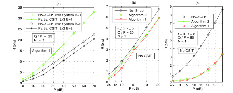
Figure 1: Numerical Results Using Two Algorithms. (a) Achievable Rates vs. P: Algorithm 1. (b) Comparison of Two Algorithms: $2\times 2$ FDPC. (c) Comparison of Two Algorithms: $3\times 2$ FDPC. (No-S-ub denotes no-interference upper-bound.)

Algorithm 2: In the previous algorithm, we minimize the upper-bound (obtained via Jensen’s Inequality) on the objective function. The key idea of this second algorithm is to solve the Karush-Kuhn-Tucker conditions for the optimization problem or in other words, to find a stationary point of the objective function.

Thus, we need to solve an equation $\frac{d}{dW}E_{H}\log|M|=0$, where $M$ is the block-partitioned matrix in (6) as referred in the derivation of Algorithm 1. For simplicity, we consider in this derivation only the case of no CSIT since the results can be easily extended to the partial-CSIT case. We start with finding differential as follows:

$$dE_{H}\log|M|=E_{H}\mathrm{tr}\{M^{-1}dM\}\hskip 5.0pt\cdots\mbox{ see \cite[cite]{[\@@bibref{}{Magnus}{}{}]}. }$$

$${}=E_{H}\mathrm{tr}\left\{M^{-1}\left[\begin{array}[]{cc}dW\Sigma_{S}W^{*}+W\Sigma_{S}(dW)^{*}&(dW)\Sigma_{S}H^{*}\\ H\Sigma_{S}(dW)^{*}&0\\ \end{array}\right]\right\}$$

$${}=2\hskip 1.0ptE_{H}\mathrm{tr}\left\{\Sigma_{S}\left[\begin{array}[]{cc}W^{*}&H^{*}\end{array}\right]M^{-1}\left[\begin{array}[]{c}dW\\ 0\\ \end{array}\right]\right\}.$$

Thus we arrive at an equation $\frac{d}{dW}E_{H}\log|M|=0\Rightarrow$

$$E_{H}(A_{1}W+A_{2}^{*}H)\Sigma_{S}=0,\mbox{ where}\left[\begin{array}[]{c}A_{1}\\ A_{2}\\ \end{array}\right]=M^{-1}\left[\begin{array}[]{c}I\\ 0\\ \end{array}\right].$$ (13)

It can be proved that without loss of generality we can consider a solution of the form $W=-(E_{H}A_{1})^{-1}E_{H}(A_{2}^{*}H)=-g(W)$ for the above equation even when $|\Sigma_{S}|=0$. This fixed-point equation for $W$ allows us to set up the following iterative algorithm.

1. Start with some initial choice for $W$, i.e., $W^{(0)}$.

2. At the $n^{th}$ iteration, set $W^{(n)}=-g(W^{(n-1)})$ with required expectations computed numerically.

3. Repeat Step 2 until the improvement in the achievable rate is negligible.

Since our optimization problem is non-convex, the algorithm does not necessarily yield the optimum solution.

Simulation 2.

It is observed, rather surprisingly, that in most of the cases, both the algorithms yield $W$s that achieve almost equal rate over the FDPC. Thus, rather than considering such cases, we include here some of the plots in which one algorithm does better than the other in terms of the achievable rate. Figs. 1(b) and 1(c) show some of these cases. However, it has not been possible to precisely characterize such cases. The main advantage of Algorithm 1 over the second is that Algorithm 1 is usually faster in terms of number of iterations required.

It would be in order here to acknowledge a limitation of these algorithms. It is observed sometimes that for systems with $t>r$, these algorithms do not yield a good solution. One such example is seen in Fig. 2 in which it seems likely to us that some improvement in R is possible in a range of $P$ = $0$ to $10$ dB. It has been puzzling that even though these algorithms solve for two different things (one minimizes an upper-bound on the objective function while other solves for the stationary point of it), both of them fail at the same time and find nearly same solutions (in terms of R).

Application to the lattice-based transmission strategies: A lattice-based transmission scheme for the MIMO FDPC with no CSIT has been proposed in [10]. The problem of determination of inflation factor also appears in the design of such a scheme, for which the paper [10] does not provide any satisfactory solution. Thus, our algorithms can be used for the design of lattice-based schemes as well.

4 High SNR Analysis

In this section, we deal with the high-SNR behavior of the achievable rate and prove some important results.

4.1 FDPC

We begin with the high-SNR scaling law of the FDPC.

Theorem 1.

The rate achievable over the no (and hence partial) CSIT FDPC using DPC scales optimally in the high-SNR regime as $\mathrm{min}(r,t)\log\mathrm{SNR}$ if the ratio $\frac{Q}{P}$ is held constant as $P\to\infty$.

Proof 2.

It is clear that the scaling factor of FDPC with partial or no CSIT is upper-bounded by $\mathrm{min}(r,t)\log\mathrm{SNR}$. We, in fact, prove that it is equal to $\mathrm{min}(r,t)\log\mathrm{SNR}$ by proving that a lower-bound on the achievable rate can achieve the before-mentioned scaling factor.

Let us consider a lower-bound obtained by using a particular choice of $W=I$.

$$R \geq E_{H}\log\frac{|\Sigma_{X}||\Sigma_{Z}+H(\Sigma_{X}+\Sigma_{S})H^{*}|}{\left|\begin{array}[]{cc}\Sigma_{X}+\Sigma_{S}&(\Sigma_{X}+\Sigma_{S})H^{*}\\ H(\Sigma_{X}+\Sigma_{S})&H(\Sigma_{X}+\Sigma_{S})H^{*}+\Sigma_{Z}\\ \end{array}\right|}$$ (16)

$$= E_{H}\log\frac{|\Sigma_{X}||\Sigma_{Z}+H(\Sigma_{X}+\Sigma_{S})H^{*}|}{\left|\begin{array}[]{cc}\Sigma_{X}+\Sigma_{S}&0\\ 0&\Sigma_{Z}\\ \end{array}\right|}$$ (19)

$$\geq E_{H}\log\left\{\frac{|\Sigma_{X}|}{|\Sigma_{X}+\Sigma_{S}|}\frac{|\Sigma_{Z}+H\Sigma_{X}H^{*}|}{|\Sigma_{Z}|}\right\},$$ (20)

where the equality in (19) follows due to row and column operations, whereas the inequality in (20) follows because $\Sigma_{X}+\Sigma_{S}\succeq\Sigma_{X}$ within partial order.

Since $\frac{Q}{P}$ is assumed to remain constant as $P\to\infty$, the first factor $\frac{|\Sigma_{X}|}{|\Sigma_{X}+\Sigma_{S}|}$ remains bounded as $P\to\infty$. The second factor $E_{H}\log\frac{|\Sigma_{Z}+H\Sigma_{X}H^{*}|}{|\Sigma_{Z}|}$ can be made to scale in the high-SNR regime as $\mathrm{min}(r,t)\log\mathrm{SNR}$, even without any CSIT, by choosing an appropriate $\Sigma_{X}$.

The theorem above proves the achievability of the largest possible scaling factor over the partial or no CSIT MIMO FDPC and in this sense, the statement of the theorem is the strongest.

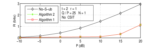
Figure 2: A Case in which Algorithms Do Not Work.

The above theorem can be further strengthened in the case of FDPC with $t\leq r$.

Theorem 3.

For the FDPC with $t\leq r$, if the ratio $\frac{Q}{P}$ is held constant, the difference $\triangle R$ between the no-interference upper-bound and the rate achievable under no (and hence partial) CSIT tends to zero as $P\to\infty$.

Proof 4.

Under the specific choice of $W=I$, we get

$$\triangle R=E_{H}\log\frac{|\Sigma_{Z}+H\Sigma_{X}H^{*}|}{|\Sigma_{Z}+H(\Sigma_{X}+\Sigma_{S})H^{*}|}-\log\frac{|\Sigma_{X}|}{|\Sigma_{X}+\Sigma_{S}|}$$

$${}=E_{H}\log\frac{|I+TH\Sigma_{X}H^{*}T^{*}|}{|I+TH(\Sigma_{X}+\Sigma_{S})H^{*}T^{*}|}-\log\frac{|\Sigma_{X}|}{|\Sigma_{X}+\Sigma_{S}|}$$

$${}=E_{H}\log\frac{|P^{-1}I+\Sigma_{X}^{\prime}H^{*}\Sigma_{Z}^{-1}H|}{|P^{-1}I+(\Sigma_{X}^{\prime}+\Sigma_{S}^{\prime})H^{*}\Sigma_{Z}^{-1}H|}-\log\frac{|\Sigma_{X}^{\prime}|}{|\Sigma_{X}^{\prime}+\Sigma_{S}^{\prime}|},$$

where $\Sigma_{Z}=T^{-1}(T^{*})^{-1}$, $\Sigma_{X}=P\Sigma_{X}^{\prime}$, $\Sigma_{S}=P\Sigma_{S}^{\prime}$, and the third equality follows from the fact that $|I+AB|=|I+BA|$ whenever products $AB$ and $BA$ are defined.

For the case of $t\leq r$, matrix $H^{*}\Sigma_{Z}^{-1}H$ is invertible. Thus, we obtain $\lim_{P\to\infty}\triangle R=0$. Therefore, the choice $W=I$ is optimal at high SNR for FDPCs with $t\leq r$.

For $t>r$ case, $\triangle R$ does not indeed to go to zero, except in some special cases.

There is a nice intuitive explanation of why $\triangle R$ tends to zero when $t\leq r$. Consider the perfect-CSIT-optimal $W$, i.e., $W=\Sigma_{X}H^{*}(H\Sigma_{X}H^{*}+\Sigma_{Z})^{-1}H$. For $t\leq r$, it can be proved that $W\to I$ as $P\to\infty$ for any value of $H$. Hence, when $t\leq r$, in the limit of high SNR, knowledge of $H$ is not required as far as determination of $W$ is concerned, and therefore, we get $\triangle R=0$ in limit. However, for the case of $t>r$, we get $W\to\Sigma_{X}^{\prime}H^{*}(H\Sigma_{X}^{\prime}H^{*})^{-1}H$ (as $P\to\infty$) which depends on the value of $H$. Hence, for FDPCs with $t>r$, even in the limit, CSIT is required for determination of $W$, and thus $\triangle R$ does not to go to zero in general.

An important implication of the above theorem is the following proposition.

Proposition 5.

For FDPCs with $t\leq r$, Costa’s choice of auxiliary RV, namely, $U=X+WS$ is optimal at high SNR even under partial or no CSIT.

Thus, for the first time the optimality of Costa’s choice of auxiliary RV is shown under partial CSIT (even though it is only in a special case).

4.2 Gaussian MIMO BC

Theorem 1 proved in the previous subsection has an important consequence on the achievable sum-rate scaling factor of the Gaussian MIMO BC with partial or no CSIT. It is now well-established that given a fixed level of partial CSIT beamforming-based multi-user transmission strategies can not achieve sum-rate scaling over the MIMO BC [11]. And thus, till now, only the single-user strategy of time-division multiple access (TDMA) was known to achieve to the sum-rate scaling. However, as the following proposition suggests, a DPC-based multi-user transmission strategy can also achieve the same.

Proposition 6.

For the Gaussian MIMO BC with $t$ transmit antennas and users with $r$ receive antenna each, a high-SNR sum-rate scaling factor of $\mathrm{min}(t,r)\log\mathrm{SNR}$ can be achieved even without any CSIT if DPC is used.

Proof 7.

If DPC is used at the transmitter, for the user encoded last, unlike other users, entire interference can be (potentially) canceled by DPC. Hence, as per Theorem 1, the achievable rate for the last user can be made to scale in the high-SNR regime as $\mathrm{min}(t,r)\log\mathrm{SNR}$.

Though TDMA can achieve the same scaling factor, this result is interesting because it is for the first time that a multi-user strategy is shown to achieve a non-zero high-SNR sum-rate scaling factor over the Gaussian MIMO BC with partial or no CSIT. Also, this proposition is in accordance with the main result and the conjecture of [12].

5 Conclusion and Future Scope

The paper proposes two good algorithmic solutions for the problem of determination of inflation factor. Apart from this, some important results are proved analytically in the high SNR regime. Our algorithmic solutions are found to work well, except in some cases as mentioned before. More efforts are required to better the performance in these cases.

References

- [1] M.Costa, “Writing on dirty paper,” IEEE Trans. Inform. Theory, vol. 29, no. 3, pp. 439–441, May 1983.
- [2] S.Gelfand and M.Pinsker, “Coding for channel with random parameters,” Problems of control and information theory, vol. 9, no. 1, pp. 19–31, 1980.
- [3] A. Bennatan and D. Burshtein, “On the fading paper achievable region of the fading MIMO broadcast channel,” in 44th annual Allerton Conference on Communication, Control and Computing, Univ. of Illinois, Sep. 2006.
- [4] W.Zhang, S. Kotagiri, and J. N. Laneman, “Writing on dirty paper with resizing and its application to quasi-static broadcast channel,” in IEEE Int. Symp. Information Theory, Nice, France, Jun. 2007, pp. 381–385.
- [5] P. Piantanida and P. Duhamel, “Dirty paper coding without channel information at the transmitter and imperfect estimation at the receiver,” in IEEE Int. Conf. Communications, Glasgow, Scotland, Jun. 2007, pp. 5406–5411.
- [6] T. Cover and M. Chiang, “Duality between channel capacity and rate distortion with two-sided state information,” IEEE Trans. Inform. Theory, vol. 48, no. 6, pp. 1629–1638, Jun. 2002.
- [7] J. Max, “Quantizing for minimum distortion,” IEEE Trans. Inform. Theory, vol. 6, no. 1, pp. 7–12, Mar. 1960.
- [8] E. Telatar, “Capacity of multi-antenna gaussian channels,” European Trans. on Telecomm., vol. 10, pp. 585–595, 1999.
- [9] J. Magnus and H. Neudecker, Matrix Differential Calculus with Applications in Statistics and Econometrics, John Wiley and Sons, Inc., 1988.
- [10] S. C. Lin, P. H. Lin, and H. Su, “Lattice coding for the vector fading paper problem,” in IEEE Inform. Theory Workshop, Tahoe City, CA, USA, Sep. 2007, pp. 78–83.
- [11] N. Jindal, “MIMO broadcast channels with finite rate feedback,” IEEE Trans. Inform. Theory, vol. 52, no. 11, pp. 5045–5060, Nov. 2006.
- [12] A. Lapidoth, S. Shamai (Shitz), and M. Wiger, “On the capacity of a MIMO fading broadcast channel with imperfect transmitter side-information,” in 43rd annual Allerton Conference on Communication, Control and Computing, Monticello, IL, Sep. 2005.