Weakly nonlinear Schrödinger equation with
random initial data

Abstract

It is common practice to approximate a weakly nonlinear wave equation through a kinetic transport equation, thus raising the issue of controlling the validity of the kinetic limit for a suitable choice of the random initial data. While for the general case a proof of the kinetic limit remains open, we report on first progress. As wave equation we consider the nonlinear Schrödinger equation discretized on a hypercubic lattice. Since this is a Hamiltonian system, a natural choice of random initial data is distributing them according to the corresponding Gibbs measure with a chemical potential chosen so that the Gibbs field has exponential mixing. The solution $\psi_{t}(x)$ of the nonlinear Schrödinger equation yields then a stochastic process stationary in $x\in\mathbb{Z}^{d}$ and $t\in\mathbb{R}$. If $\lambda$ denotes the strength of the nonlinearity, we prove that the space-time covariance of $\psi_{t}(x)$ has a limit as $\lambda\to 0$ for $t=\lambda^{-2}\tau$, with $\tau$ fixed and $|\tau|$ sufficiently small. The limit agrees with the prediction from kinetic theory.

1 Introduction

The nonlinear Schrödinger equation (NLS) governs the evolution of a complex valued wave field $\psi:\mathbb{R}\times\mathbb{Z}^{d}\to\mathbb{C}$ and reads

$$\textrm{i}\frac{\textrm{d}}{\textrm{d}t}\psi_{t}(x)=\sum_{y\in\mathbb{Z}^{d}}\alpha(x-y)\psi_{t}(y)+\lambda|\psi_{t}(x)|^{2}\psi_{t}(x)\,.$$ (1.1)

Here $\alpha(x)$ are the “hopping amplitudes” and we assume that they satisfy

• $\alpha:\mathbb{Z}^{d}\to\mathbb{R}$, $\alpha(x)=\alpha(-x)$.

• $|\alpha|$ has an exponentially decreasing upper bound.

We consider only the dispersive case $\lambda\geq 0$. Usually the NLS is studied in the continuum setting, where $\mathbb{Z}^{d}$ is replaced by $\mathbb{R}^{d}$ and the linear term is $\Delta\psi_{t}(x)$. It will become evident later on why for our purposes the spatial discretization is a necessity.

The NLS is a Hamiltonian system. To see this, we define the canonical degrees of freedom $q_{x},p_{x}\in{\mathbb{R}}$, $x\in\mathbb{Z}^{d}$, via $\psi(x)=(q_{x}+{\rm i}p_{x})/\sqrt{2}$. Their Hamiltonian function is obtained by substitution in

$$H(\psi)=\sum_{x,y\in\mathbb{Z}^{d}}\alpha(x-y)\psi(x)^{\ast}\psi(y)+\tfrac{1}{2}\lambda\sum_{x\in\mathbb{Z}^{d}}|\psi(x)|^{4}\,.$$ (1.2)

It is easy to check that the corresponding equations of motion,

$$\frac{\textrm{d}}{\textrm{d}t}q_{x}=\frac{\partial}{\partial p_{x}}H\,,\quad\frac{\textrm{d}}{\textrm{d}t}p_{x}=-\frac{\partial}{\partial q_{x}}H\,,$$ (1.3)

are identical to the NLS. In particular, we conclude that the energy is conserved, $H(\psi_{t})=H(\psi_{0})$ for all $t\in\mathbb{R}$. Also the $\ell_{2}$-norm is conserved, in this context also referred to as particle number $N$,

$$N(\psi)=\sum_{x\in\mathbb{Z}^{d}}|\psi(x)|^{2}\,,\quad N(\psi_{t})=N(\psi_{0})\textrm{ for all }t\in\mathbb{R}\,.$$ (1.4)

Because of energy conservation law, if $H(\psi_{0})<\infty$, then the Cauchy problem for (1.1) has a unique global solution. We refer to [22] for a more detailed information on the NLS.

In this work we are interested in random initial data. From a statistical physics point of view a very natural choice is to take the initial $\psi$-field to be distributed according to a Gibbs measure for $H$ and $N$, which physically means that the wave field is in thermal equilibrium. Somewhat formally the Gibbs measure is defined through

$$\frac{1}{Z}\exp\big{[}-\beta\big{(}H(\psi)-\mu N(\psi)\big{)}\big{]}\prod_{x}\left[{\rm d}\bigl{(}{\rm Re\,}\psi(x)\bigr{)}{\rm d}\bigl{(}{\rm Im\,}\psi(x)\bigr{)}\right].$$ (1.5)

Here $\beta>0$ is the inverse temperature and $\mu\in\mathbb{R}$ the chemical potential. The partition function $Z$ is a constant chosen so that (1.5) is a probability measure. To properly define the Gibbs measure one has to restrict (1.5) to some finite box $\Lambda\subset\mathbb{Z}^{d}$, which yields a well-defined probability measure $\mathbb{P}^{\lambda}_{\beta,\mu,\Lambda}$ on $\mathbb{C}^{|\Lambda|}$. The Gibbs probability measure $\mathbb{P}^{\lambda}_{\beta,\mu}$ on $\mathbb{Z}^{d}$ is then obtained in the limit $\Lambda\nearrow\mathbb{Z}^{d}$. The existence of this limit is a well-studied problem [15]. If $\lambda$ is sufficiently small and $\mu$ sufficiently negative, then the Gibbs measure $\mathbb{P}^{\lambda}_{\beta,\mu}$ exists. The random field $\psi(x)$, $x\in\mathbb{Z}^{d}$, distributed according to $\mathbb{P}^{\lambda}_{\beta,\mu}$, is stationary with a rapid decay of correlations. It is also gauge invariant in the sense that $\psi(x)=\mathrm{e}^{i\theta}\psi(x)$ in distribution for any $\theta\in[0,2\pi]$.

Of course, $\mathbb{P}^{\lambda}_{\beta,\mu}$-almost surely it holds $H(\psi)=\infty$ and $N(\psi)=\infty$. Thus one has to define solutions for the NLS with initial data of infinite energy. This has been accomplished for standard anharmonic Hamiltonian systems by Lanford, Lebowitz, and Lieb [14], who prove existence and uniqueness under a suitable growth condition at infinity for the initial data. These arguments extend to the Hamiltonian system (1.3). It remains to prove that the so-defined infinite volume dynamics is well approximated by the finite volume dynamics with periodic boundary conditions. Very likely such a result can be achieved using the methods developed in [4]. For our purposes it is more convenient to circumvent the issue by proving estimates which are uniform in the volume.

Let us briefly comment why the more conventional continuum NLS,

$${\rm i}\frac{\partial}{\partial t}u(x,t)=-\Delta_{x}u(x,t)+\lambda\int_{{\mathbb{R}}^{d}}\!{\rm d}y\,|u(y,t)|^{2}V(y-x)u(x,t),\quad x\in{\mathbb{R}}^{d},\ t\in{\mathbb{R}}\,,$$ (1.6)

poses additional difficulties. The Gibbs measure at finite volume is a perturbed Gaussian measure which is singular at short distances. Thus the construction of the dynamics requires an effort. Furthermore, the limit $V(x)\to\delta(x)$ is a fundamental problem of constructive quantum field theory and is known to be difficult [9]. To establish the existence of the dynamics for such singular initial data has not even been attempted.

In the present context the most basic quantity is the stationary covariance

$$\mathbb{E}^{\lambda}_{\beta,\mu}\big{(}\psi_{0}(x_{0})^{\ast}\psi_{t}(x)\big{)}=F^{\lambda}_{2}(x-x_{0},t)\,,$$ (1.7)

where $\mathbb{E}^{\lambda}_{\beta,\mu}$ denotes expectation with respect to $\mathbb{P}^{\lambda}_{\beta,\mu}$. The existence of such a function $F^{\lambda}_{2}$ follows from the translation invariance of the measure, and one would like to know its qualitative dependence on $x,t$. For deterministic infinitely extended Hamiltonian systems, such as the NLS, establishing the qualitative behavior of equilibrium time correlations is known to be an extremely difficult problem with very few results available, despite intense efforts. For linear systems one has an explicit solution in Fourier space, see below. But already for completely integrable systems, like the Toda chain, not much is known about time correlations in thermal equilibrium.

It is instructive first to discuss the linear case, $\lambda=0$, for which purpose we introduce Fourier transforms. For $f:\mathbb{Z}^{d}\to\mathbb{C}$ let us denote its Fourier transform by

$$\hat{f}(k)=\sum_{x\in\mathbb{Z}^{d}}f(x)\textrm{e}^{-\textrm{i}2\pi k\cdot x}\,,$$ (1.8)

$k\in\mathbb{R}$, and the inverse Fourier transform by

$$\tilde{g}(x)=\int_{\mathbb{T}^{d}}\textrm{d}k\,g(k)\textrm{e}^{\textrm{i}2\pi k\cdot x}$$ (1.9)

with $\mathbb{T}^{d}=[0,1]^{d}$, a parametrization of the $d$-dimensional torus. (We will use arithmetic relations on ${\mathbb{T}}^{d}$. These are defined using the arithmetic induced on the torus via its definition as equivalence classes ${\mathbb{R}}^{d}/{\mathbb{Z}}^{d}$, i.e., by using “periodic boundary conditions”.) In particular, we set

$$\omega(k)=\hat{\alpha}(k),\quad k\in{\mathbb{T}}^{d}\,.$$ (1.10)

The function $\omega$ is the dispersion relation of our discretized linear Schrödinger equation. It follows from the assumptions on $\alpha$ that

• $\omega:\mathbb{T}^{d}\to\mathbb{R}$ and its periodic extension is a real analytic function.

• $\omega(k)=\omega(-k)$.

In Fourier space the energy is given by

$$H(\psi)=\int_{\mathbb{T}^{d}}\textrm{d}k\,\omega(k)|\hat{\psi}(k)|^{2}$$

$$\quad+\tfrac{1}{2}\lambda\int_{(\mathbb{T}^{d})^{4}}\textrm{d}k_{1}\textrm{d}k_{2}\textrm{d}k_{3}\textrm{d}k_{4}\delta(k_{1}+k_{2}-k_{3}-k_{4})\hat{\psi}(k_{1})^{\ast}\hat{\psi}(k_{2})^{\ast}\hat{\psi}(k_{3})\hat{\psi}(k_{4})\,,$$ (1.11)

where $\delta$ is a formal Dirac $\delta$-function, used here to simplify the notation for the convolution integral. Clearly, $H(\psi)\geq(\inf_{k}\omega(k))N(\psi)$. The NLS after Fourier transform reads

$$\frac{\textrm{d}}{\textrm{d}t}\hat{\psi}_{t}(k_{1})=-\textrm{i}\omega(k_{1})\hat{\psi}_{t}(k_{1})-\textrm{i}\lambda\int\textrm{d}k_{2}\textrm{d}k_{3}\textrm{d}k_{4}\delta(k_{1}+k_{2}-k_{3}-k_{4})$$

$$\qquad\times\hat{\psi}_{t}(k_{2})^{\ast}\hat{\psi}_{t}(k_{3})\hat{\psi}_{t}(k_{4})\,.$$ (1.12)

For $\lambda=0$, $\mathbb{P}^{0}_{\beta,\mu}$ is a Gaussian measure with mean zero and covariance

$$\mathbb{E}^{0}_{\beta,\mu}\big{(}\psi(0)^{\ast}\psi(x)\big{)}=F^{0}_{2}(x,0)=\int_{\mathbb{T}^{d}}\textrm{d}k\big{(}\beta(\omega(k)-\mu)\big{)}^{-1}\textrm{e}^{\textrm{i}2\pi k\cdot x}\,,$$ (1.13)

provided $\mu<\inf_{k}\omega(k)$. Under our assumptions on $\omega$ the Gaussian field has exponential mixing. For the time-dependent equilibrium covariance one obtains

$$F^{0}_{2}(x,t)=\int_{\mathbb{T}^{d}}\textrm{d}k\big{(}\beta(\omega(k)-\mu)\big{)}^{-1}\textrm{e}^{\textrm{i}2\pi k\cdot x}\textrm{e}^{-\textrm{i}\omega(k)t}\,.$$ (1.14)

Clearly, $F^{0}_{2}(x,t)$ is a solution of the linear wave equation for exponentially localized initial data and thus spreads dispersively.

If $\lambda>0$, as general heuristics the nonlinearity should induce an exponential damping of $F^{\lambda}_{2}$. The physical picture is based on excitations of wave modes which interact weakly and are damped through collisions. Approximate theories have been developed in the context of phonon physics and wave turbulence, see e.g. [10, 23]. To mathematically establish such a time-decay is completely out of reach, at present, whatever the choice of the nonlinear wave equation.

To make some progress we will investigate here the regime of small nonlinearity, $\lambda\ll 1$. The idea is not to aim for results which are valid globally in time, but rather to consider the first time scale on which the effect of the nonlinearity becomes visible. For small $\lambda$ the rate of collision for two resonant waves is of order $\lambda^{2}$. Therefore, the nonlinearity is expected to show up on a time scale $\lambda^{-2}$. This suggests to study the limit

$$F^{\lambda}_{2}(x,\lambda^{-2}t)\,,\quad\textrm{as }\lambda\to 0\,.$$ (1.15)

Note that the location $x$ is not scaled. For this limit to exist, one has to remove the oscillating phase resulting from (1.14), which on the speeded-up time scale is rapidly oscillating, of order $\lambda^{-2}$. In fact, a second rapidly oscillating phase of order $\lambda^{-1}$ will show up, which also has to be removed. Under suitable conditions on $\omega$, we will prove that $F^{\lambda}_{2}(x,\lambda^{-2}t)$, with the removals just mentioned, has a limit for $\lambda\to 0$, at least for $|t|\leq t_{0}$ with some suitable $t_{0}>0$. The limit function indeed exhibits exponential damping.

A similar result has been obtained a long time ago for a system of hard spheres in equilibrium and at low, but fixed, density [2]. There the small parameter is the density rather than the strength $\lambda$ of the nonlinearity. But the over-all philosophy is the same. To establish the decay of time-correlations in equilibrium at a fixed low density is an apparently very hard problem. Therefore, one looks for the first time scale on which the collisions between hard spheres have a visible effect. By fiat, hard spheres remain well localized in space, and on the time scale of interest only a finite number of collisions per particle are taken into account. In contrast, waves tend to delocalize through collisions. This is the reason why the problem under study has remained open. Our resolution uses techniques totally different from [2].

The limit $\lambda\to 0$, $t=\lambda^{-2}\tau$ with $\tau$ fixed, together with a possible rescaling of space by a factor $\lambda^{-2}$, is called kinetic limit, because the limit object is governed by a kinetic type transport equation. Formal derivations are discussed extensively in the literature, e.g., see [12, 18]. On the mathematical side, Erdős and Yau [8] study in great detail the linear Schrödinger equation with a random potential, extended to even longer time scales in [6, 7]. The discretized wave equation with a random index of refraction is covered in [16]. For nonlinear wave equations the only related study is by Benedetto et al. [3] on the dynamics of weakly interacting quantum particles. They transform to multipoint Wigner functions, which leads to an expansion somewhat different from the one used here. We refer to [17] for a comparison. As in our contribution, Benedetto et al. have to analyze the asymptotics of high-dimensional oscillatory integrals. But in contrast, they have no control on the error term in the expansion.

Before closing the introduction, we owe the reader some explanations why a seemingly perturbative result requires so many pages for its proof. From the solution to (1.1) one can regard $\psi_{t}(x)$ as some functional $\mathcal{F}_{x,t}$ of the initial field $\psi$,

$$\psi_{t}(x)=\mathcal{F}_{x,t}(\psi)\,.$$ (1.16)

For given $t$ it depends only very little on those $\psi(y)$’s for which $|y-x|\gg t$. To make progress it seems necessary to first average the initial conditions over $\psi(x_{0})^{\ast}\mathbb{P}^{\lambda}_{\beta,\mu}$ so that subsequently one can control the limit $\lambda\to 0$ with $t=\lambda^{-2}\tau$, $\tau>0$. Such an average can be accomplished by writing $\mathcal{F}_{x,t}$ as a power series in $\psi$, which is done through the Duhamel formula. For any $n\geq 1$ we write

$$\prod^{n}_{j=1}\textrm{e}^{\textrm{i}2\pi\sigma_{j}\omega(k_{j})t}\hat{\psi}_{t}(k_{j},\sigma_{j})=\prod^{n}_{j=1}\hat{\psi}_{0}(k_{j},\sigma_{j})+\int^{t}_{0}\textrm{d}s\frac{\textrm{d}}{\textrm{d}s}\prod^{n}_{j=1}\textrm{e}^{\textrm{i}2\pi\sigma_{j}\omega(k_{j})s}\hat{\psi}_{s}(k_{j},\sigma_{j})\,.$$ (1.17)

Here $\sigma_{j}\in\{\pm 1\}$ and $\hat{\psi}_{t}(k,1)=\hat{\psi}_{t}(k)$, $\hat{\psi}_{t}(k,-1)=\hat{\psi}_{t}(-k)^{\ast}$, $\hat{\psi}_{0}(k)=\hat{\psi}(k)$. Using the product rule and the equations of motion (1) yields a formula relating the $n$:th moment at time $t$ to the time-integral of a sum over $(n+2)$:th moments at time $s$. Iterating this equation leads to a (formal) series representation

$$\hat{\psi}_{t}(k)=\sum^{\infty}_{n=1}\mathcal{P}^{n}_{k,t}(\hat{\psi})\,,$$ (1.18)

where $\mathcal{P}^{n}_{k,t}$ is a sum/integral over monomials of order $n$ in $\hat{\psi}$ and $\hat{\psi}^{\ast}$. Since each time-derivative increases the degree of the monomial by two, we have

$$\delta(k^{\prime}-k)\sum_{x\in\mathbb{Z}^{d}}\textrm{e}^{-\textrm{i}2\pi k\cdot x}\mathbb{E}^{\lambda}_{\beta,\mu}\big{(}\psi(0)^{\ast}\psi_{t}(x)\big{)}=\sum^{\infty}_{n=0}\mathbb{E}^{\lambda}_{\beta,\mu}\big{(}\hat{\psi}(k^{\prime})^{\ast}\mathcal{P}^{2n+1}_{k,t}(\hat{\psi})\big{)}\,.$$ (1.19)

The first difficulty arises from the fact that the sum in (1.19) does not converge absolutely for any $t$. Very roughly, $\mathcal{P}^{n}_{k,t}$ is a sum of $n!$ terms of equal size. The iterated time-integration yields a factor $t^{n}/n!$. However, for the approximately Gaussian average the $n$:th moment grows also as $n!$. To be able to proceed one has to stop the series expansion at some large $N$ which depends on $\lambda$. A similar situation was encountered by Erdős and Yau [8] in their study of the Schrödinger equation with a weak random potential. We will use the powerful Erdős-Yau techniques as a guideline for handling the series in (1.19).

The stopping of the series expansion will leave a remainder term containing the full original time-evolution. Erdős and Yau control the error term in essence by unitarity of the time-evolution. For the NLS mere conservation of $N(\psi)$ will not suffice. Instead, we use stationarity of $\psi_{t}(x)$. In wave turbulence [23] one is also interested in non-stationary initial measures, e.g., in Gaussian measures with a covariance different from $(\beta(\omega(k)-\mu))^{-1}$. For such initial data we have no idea how to control the error term, while other parts of our proof apply unaltered.

The central difficulty resides in $\mathbb{E}^{\lambda}_{\beta,\mu}\big{(}\hat{\psi}(k^{\prime})^{\ast}\mathcal{P}^{2n+1}_{k,t}(\hat{\psi})\big{)}$ which is a sum of rather explicit, but high-dimensional, dimension $n(1+3d)+d$, oscillatory integrals. On top, because of the $\delta$-function in (1), the integrand is restricted to a non-trivial linear subspace. In the limit $\lambda\to 0$, $t=\lambda^{-2}\tau$, $\tau>0$, only a few oscillatory integrals have a non-zero limit. Summing up these leading oscillatory integrals results in the anticipated exponential damping. The major task of our paper is to discover an iterative structure in all remaining oscillatory integrals, in a way which allows for an estimate in terms of a few basic “motives”. Each of these subleading integrals is shown to contain at least one motive whose appearance leads to an extra fractional power of $\lambda$, thereby ensuring a zero limit.

In Section 2.1 we first give the mathematical definition of the above system in finite volume, and state in Section 2.2 the assumptions and main results. Their connection to kinetic theory is discussed in Section 2.3. The proof of the main result is contained in the remaining sections: we derive a suitable time-dependent perturbation expansion in Section 3, and develop a graphical language to describe the large, but finite, number of terms in the expansion in Section 4. The analysis of the oscillatory integrals in the expansion is contained in Sections 5–9. More detailed outline of the technical structure of the proof can be found in Section 3.1. The estimates are collected together and the limit of the non-zero terms is computed in Section 10 where we complete the proof of the main theorem. In an Appendix, we show that the standard nearest neighbor couplings in $d\geq 4$ dimensions lead to dispersion relations satisfying all assumptions of the main theorem.

Acknowledgments. We would like to thank László Erdős and Horng-Tzer Yau for many illuminating discussions on the subject. The research of J. Lukkarinen was supported by the Academy of Finland.

2 Kinetic limit and main results

2.1 Finite volume dynamics

To properly define expectations such as (1.7), one has to go through a finite volume construction, which will be specified in this subsection.

Let

$$L\geq 2\,,\quad\Lambda=\{0,1,\ldots,L-1\}^{d}\,,$$ (2.1)

the dimension $d$ an arbitrary positive integer. We apply periodic boundary conditions on $\Lambda$, and let $[x]=x\bmod L\in\Lambda$ for all $x\in\mathbb{Z}^{d}$. Fourier transform of $f:\Lambda\to\mathbb{C}$ is denoted by $\hat{f}:\Lambda^{*}\to\mathbb{C}$, with the dual lattice $\Lambda^{*}=\{0,\frac{1}{L},\ldots,\frac{L-1}{L}\}^{d}$ and with

$$\hat{f}(k)=\sum_{x\in\Lambda}f(x)\textrm{e}^{-\textrm{i}2\pi k\cdot x}$$ (2.2)

for all $k\in\Lambda^{*}$ (or for all $k\in(\mathbb{Z}/L)^{d}$, which yields the periodic extension of $\hat{f}$). The inverse transform is given by

$$\tilde{g}(x)=\frac{1}{|\Lambda|}\sum_{k\in\Lambda^{*}}g(k)\textrm{e}^{\textrm{i}2\pi k\cdot x}\,,$$ (2.3)

where $|\Lambda|=L^{d}$. For all $x\in\Lambda$, it holds $\tilde{{\hat{f}}}(x)=f(x)$. The arithmetic operations on $\Lambda$ are done periodically, identifying it as a parametrization of $\mathbb{Z}_{L}^{d}$, the cyclic group of $L$ elements (for instance, for $x,y\in\Lambda$, we have then $x+y=[x+y]$ and $-x=[-x]$.) Similarly, $\Lambda^{*}$ is identified as a subset of the $d$-torus $\mathbb{T}^{d}$.

We will use the short-hand notations

$$\int_{\Lambda^{*}}\textrm{d}k\,\cdots=\frac{1}{|\Lambda|}\sum_{k\in\Lambda^{*}}\cdots\,,$$ (2.4)

and

$$\langle f,\psi\rangle=\sum_{x\in\Lambda}f(x)^{\ast}\psi(x)\,,$$ (2.5)

as well as the similar but unrelated notation for “regularized” absolute values

$$\langle x\rangle=\sqrt{1+x^{2}},\qquad\text{for all }x\in{\mathbb{R}}\,.$$ (2.6)

Let us also denote the limit $L\to\infty$ by $\Lambda\to\infty$. Let $\omega:\mathbb{T}^{d}\to\mathbb{R}$ be defined as in (1.10). For the finite volume, we introduce the periodized $\alpha_{\Lambda}$ through

$$\alpha_{\Lambda}(x)=\int_{\Lambda^{*}}\!\textrm{d}k\,\textrm{e}^{\textrm{i}2\pi x\cdot k}\omega(k)=\frac{1}{|\Lambda|}\sum_{k\in\Lambda^{*}}\textrm{e}^{\textrm{i}2\pi x\cdot k}\omega(k).$$ (2.7)

Clearly, $\alpha_{\Lambda}\in\mathbb{R}$ and $\alpha_{\Lambda}(-x)=\alpha_{\Lambda}(x)$ for all $x\in\Lambda$.

After these preparations, we define the finite volume Hamiltonian for $\psi:\Lambda\to\mathbb{C}$ by

$$H_{\Lambda}(\psi)=\sum_{x,y\in\Lambda}\alpha_{\Lambda}(x-y)\psi(x)^{*}\psi(y)+\tfrac{1}{2}\lambda\sum_{x\in\Lambda}|\psi(x)|^{4}$$

$$\quad=\int_{\Lambda^{*}}\textrm{d}k\,\omega(k)|\hat{\psi}(k)|^{2}$$

$$\qquad+\tfrac{1}{2}\lambda\int_{(\Lambda^{*})^{4}}\!\!\!\textrm{d}k_{1}\textrm{d}k_{2}\textrm{d}k_{3}\textrm{d}k_{4}\,\delta_{\Lambda}(k_{1}+k_{2}-k_{3}-k_{4})\hat{\psi}(k_{1})^{*}\hat{\psi}(k_{2})^{*}\hat{\psi}(k_{3})\hat{\psi}(k_{4})\,,$$ (2.8)

where $\lambda\geq 0$ and $\delta_{\Lambda}:(\mathbb{Z}/L)^{d}\to\mathbb{R}$ is the following discrete $\delta$-function

$$\delta_{\Lambda}(k)=|\Lambda|\mathbbm{1}(k\bmod 1=0).$$ (2.9)

Here ${\mathbbm{1}}$ denotes a generic characteristic function: ${\mathbbm{1}}(P)=1$, if the condition $P$ is true, and ${\mathbbm{1}}(P)=0$ otherwise. $H_{\Lambda}(\psi)\geq c\|\psi\|^{2}_{2}$ for all $\psi$, with $c=\inf_{k}\omega(k)>-\infty$ and $\|\psi\|_{2}$ denoting the $\ell_{2}(\Lambda)$-norm.

Introducing, as before, the canonical conjugate pair $q_{x},p_{x}\in{\mathbb{R}}$ through $\psi(x)=(q_{x}+{\rm i}p_{x})/\sqrt{2}$, and then applying the evolution equations associated to $H_{\Lambda}$, we find that $\psi_{t}(x)$ satisfies the finite volume discrete NLS

$$\textrm{i}\frac{\textrm{d}}{\textrm{d}t}\psi_{t}(x)=\sum_{y\in\Lambda}\alpha_{\Lambda}(x-y)\psi_{t}(y)+\lambda|\psi_{t}(x)|^{2}\psi_{t}(x)\,.$$ (2.10)

The Fourier-transform $\hat{\psi}_{t}(k)$ satisfies the evolution equation

$$\frac{{\rm d}}{{\rm d}t}\hat{\psi}_{t}(k_{1})=-{\rm i}\omega(k_{1})\hat{\psi}_{t}(k_{1})$$

$$\quad-{\rm i}\lambda\int_{(\Lambda^{*})^{3}}\!\!{\rm d}k_{2}{\rm d}k_{3}{\rm d}k_{4}\,\delta_{\Lambda}(k_{1}+k_{2}-k_{3}-k_{4})\hat{\psi}_{t}(k_{2})^{*}\hat{\psi}_{t}(k_{3})\hat{\psi}_{t}(k_{4}).$$ (2.11)

The evolution equations have a continuously differentiable solution for all $t\in{\mathbb{R}}$ and for any given initial conditions $\psi_{0}\in{\mathbb{C}\hskip 0.21529pt}^{\Lambda}$, which follows by a standard fixed point argument and the conservation laws stated below. The energy $H_{\Lambda}(\psi)$ is naturally conserved by the time-evolution. In addition, for all $x$,

$$\frac{{\rm d}}{{\rm d}t}|\psi_{t}(x)|^{2}=-{\rm i}\sum_{y\in\Lambda}\alpha_{\Lambda}(x-y)\left(\psi_{t}(x)^{*}\psi_{t}(y)-\psi_{t}(y)^{*}\psi_{t}(x)\right).$$ (2.12)

The right hand side sums to zero if we sum over all $x\in\Lambda$. Therefore, for $t\in{\mathbb{R}}$,

$$\|\psi_{t}\|_{2}^{2}=\sum_{x\in\Lambda}|\psi_{t}(x)|^{2}=\|\psi_{0}\|_{2}^{2}\,,$$ (2.13)

and thus also $\|\psi_{t}\|_{2}$ is a constant of motion.

The initial field is taken to be distributed according to the finite volume Gibbs measure as explained in the introduction. We assume that its parameters are fixed to some values satisfying $\beta>0$ and $\mu<\inf_{k}\omega(k)$, and we drop the dependence on these parameters from the notation. Then the Gibbs measure is

$$\int_{{\mathbb{C}\hskip 0.1507pt}^{\Lambda}}\mathbb{P}_{\Lambda}^{\lambda}({\rm d}\psi)f(\psi)=\frac{1}{Z_{\Lambda}^{\lambda}}\int_{({\mathbb{R}}^{2})^{\Lambda}}\prod_{x\in\Lambda}\left[{\rm d}({\rm Re\,}\psi(x))\,{\rm d}({\rm Im\,}\psi(x))\right]{\rm e}^{-\beta(H_{\Lambda}(\psi)-\mu\|\psi\|^{2})}f(\psi)\,.$$ (2.14)

Expectation values with respect to the finite volume, perturbed measure $\mathbb{P}_{\Lambda}^{\lambda}$ are denoted by ${\mathbb{E}}^{\lambda}_{\Lambda}$. Taking the limits $\Lambda\to\infty$ and $\lambda\to 0$ leads to a Gaussian measure. It is defined via its covariance function which has a Fourier transform

$$W(k)=\hat{F}_{2}^{0}(k,0)=\frac{1}{\beta(\omega(k)-\mu)}\,.$$ (2.15)

We denote expectations over this Gaussian measure by ${\mathbb{E}}^{0}$. Note that by the translation invariance of the finite volume Gibbs measure, there always exists a function $W^{\lambda}_{\Lambda}:\Lambda^{*}\to{\mathbb{C}\hskip 0.21529pt}$ such that for all $k,k^{\prime}\in\Lambda^{*}$,

$${\mathbb{E}}^{\lambda}_{\Lambda}[\hat{\psi}(k)^{*}\hat{\psi}(k^{\prime})]=\delta_{\Lambda}(k-k^{\prime})W^{\lambda}_{\Lambda}(k)\,.$$ (2.16)

Since the energy and norm are conserved, the Gibbs measure is time stationary. In other words, for all $t$ and any integrable $f$

$${\mathbb{E}}^{\lambda}_{\Lambda}[f(\psi_{t})]={\mathbb{E}}^{\lambda}_{\Lambda}[f(\psi_{0})].$$ (2.17)

In addition, since the dynamics and the Gibbs measure are invariant under periodic translations of $\Lambda$, under $\mathbb{P}^{\lambda}_{\Lambda}$ the stochastic process $(x,t)\mapsto\psi_{t}(x)$ is stationary jointly in space and time.

2.2 Main results

We have to impose two types of assumptions. Those in Assumption 2.2 are conditions on the dispersion relation $\omega$. Assumption 2.1 is concerned with a specific form of the clustering of the Gibbs measure. In each case we comment on their current status.

Assumption 2.1 (Equilibrium correlations)

Let $\beta>0$ and $\mu<\inf_{k}\omega(k)$ be given. We take the initial conditions $\psi_{0}$ to be distributed according to the Gibbs measure $\mathbb{P}_{\Lambda}^{\lambda}$ which is assumed to be $\ell_{1}$-clustering in the following sense: We assume that there exists $\lambda_{0}>0$ and $c_{0}>0$, independent of $n$, such that for $0<\lambda\leq\lambda_{0}$ and all $n\geq 4$ one has the following bound for the fully truncated correlation functions (i.e., cumulants)

$$\sup_{\Lambda,\sigma\in\{\pm 1\}^{n}}\sum_{x\in\Lambda^{n}}{\mathbbm{1}}(x_{1}=0)\Bigl{|}{\mathbb{E}}^{\lambda}_{\Lambda}\Bigl{[}\prod_{i=1}^{n}\psi(x_{i},\sigma_{i})\Bigr{]}^{\rm trunc}\Bigr{|}\leq\lambda(c_{0})^{n}n!\,,$$ (2.18)

where $\psi(x,1)=\psi(x)$, $\psi(x,-1)=\psi(x)^{*}$. We also assume a comparable convergence of the two-point correlation functions for $0<\lambda\leq\lambda_{0}$,

$$\limsup_{\Lambda\to\infty}\sum_{\|x\|_{\infty}\leq L/2}\left|{\mathbb{E}}^{\lambda}_{\Lambda}[\psi(0)^{*}\psi(x)]-{\mathbb{E}}^{0}[\psi(0)^{*}\psi(x)]\right|\leq\lambda 2(c_{0})^{2}\,.$$ (2.19)

In the present proof, valid for $d\geq 4$, we do not use the full strength of the bound in (2.18), namely, we could omit the prefactor $\lambda$. However, the prefactor could be needed in any proof which concerns $d\leq 3$. In contrast, we do make use of the prefactor in (2.19). The second condition can equivalently be recast in terms of $W$ as

$$\limsup_{\Lambda\to\infty}\sum_{\|x\|_{\infty}\leq L/2}\left|\widetilde{W}^{\lambda}_{\Lambda}(x)-\widetilde{W}(x)\right|\leq\lambda 2(c_{0})^{2}\,.$$ (2.20)

Technically, Assumption 2.1 refers to the clustering of a weakly coupled massive two-component $\lambda\phi^{4}$-theory. Such problems have a long tradition in equilibrium statistical mechanics and are handled through cluster expansions, e.g., see [19, 20]. The difficulty with Assumption 2.1 resides in the precise $n$- and $\lambda$-dependence of the bounds. Motivated by our work, the issue was reinvestigated for the equilibrium measure (2.14) in the contribution of Abdesselam, Procacci, and Scoppola [1], in which they prove Assumption 2.1 for hopping amplitudes of finite range and with zero boundary conditions, i.e., setting $\psi(x)=0$ for $x\notin\Lambda$. The authors ensure us that their results remain valid also for periodic boundary conditions, thereby establishing Assumption 2.1 for a large class of hopping amplitudes.

For the main theorem we will need properties of the linear dynamics, $\lambda=0$, which can be thought of as implicit conditions on $\omega$.

Assumption 2.2 (Dispersion relation)

Suppose $d\geq 4$, and $\omega:{\mathbb{T}}^{d}\to{\mathbb{R}}$ satisfies all of the following:

• The periodic extension of $\omega$ is real-analytic and $\omega(-k)=\omega(k)$.

• ($\ell_{3}$-dispersivity). Let us consider the free propagator

  $$p_{t}(x)=\int_{{\mathbb{T}}^{d}}\!{\rm d}k\,{\rm e}^{{\rm i}2\pi x\cdot k}{\rm e}^{-{\rm i}t\omega(k)}\,.$$ (2.21)

  We assume that there are $C,\delta>0$ such that for all $t\in{\mathbb{R}}$,

  $$\|p_{t}\|_{3}^{3}=\sum_{x\in{\mathbb{Z}}^{d}}|p_{t}(x)|^{3}\leq C\langle t\rangle^{-1-\delta}\,.$$ (2.22)

• (constructive interference). There exists a set $M^{\rm sing}\subset{\mathbb{T}}^{d}$ consisting of a union of a finite number of closed, one-dimensional, smooth submanifolds, and a constant $C$ such that for all $t\in{\mathbb{R}}$, $k_{0}\in{\mathbb{T}}^{d}$, and $\sigma\in\{\pm 1\}$,

  $$\Bigl{|}\int_{{\mathbb{T}}^{d}}\!{\rm d}k\,{\rm e}^{-{\rm i}t(\omega(k)+\sigma\omega(k-k_{0}))}\Bigr{|}\leq\frac{C\langle t\rangle^{-1}}{d(k_{0},M^{\rm sing})}\,,$$ (2.23)

  where $d(k_{0},M^{\rm sing})$ is the distance (with respect to the standard metric on the $d$-torus, ${\mathbb{R}}^{d}/{\mathbb{Z}}^{d}$) of $k_{0}$ from $M^{\rm sing}$.

• (crossing bounds). Define for $t_{0},t_{1},t_{2}\in{\mathbb{R}}$, $u_{1},u_{2}\in{\mathbb{T}}^{d}$, and $x\in{\mathbb{Z}}^{d}$,

  $$K(x;t_{0},t_{1},t_{2},u_{1},u_{2})=\int_{{\mathbb{T}}^{d}}\!{\rm d}k\,{\rm e}^{{\rm i}2\pi x\cdot k}{\rm e}^{-{\rm i}(t_{0}\omega(k)+t_{1}\omega(k+u_{1})+t_{2}\omega(k+u_{2}))}\,.$$ (2.24)

  We assume that there is a measurable function $F^{\rm cr}:{\mathbb{T}}^{d}\times{\mathbb{R}}_{+}\to[0,\infty]$ so that constants $0<\gamma\leq 1$, $c_{1},c_{2}$, for the following bounds can be found.

  1. For any $u_{i}\in{\mathbb{T}}^{d}$, $\sigma_{i}\in\{\pm 1\}$, $i=1,2,3$, and $0<\beta\leq 1$, the following bounds are satisfied:

     $$\int_{-\infty}^{\infty}\!{\rm d}t\,\|p_{t}\|_{3}^{2}\int_{-\infty}^{\infty}\!{\rm d}s\,{\rm e}^{-\beta|s|}\|K(t,\sigma_{1}s,\sigma_{2}s,u_{1},u_{2})\|_{3}\leq\beta^{\gamma-1}F^{\rm cr}(u_{2}-u_{1};\beta)\,,$$ (2.25)

     $$\int_{-\infty}^{\infty}\!{\rm d}t\int_{-\infty}^{\infty}\!{\rm d}s\,{\rm e}^{-\beta|s|}\prod_{i=1}^{3}\|K(t,\sigma_{i}s,0,u_{i},0)\|_{3}$$

     $$\quad\leq\beta^{\gamma-1}F^{\rm cr}(u_{n};\beta),\quad\text{for any }n\in\{1,2,3\}\,.$$ (2.26)

  2. For all $0<\beta\leq 1$ we have

     $$\int_{{\mathbb{T}}^{d}}{\rm d}k\,F^{\rm cr}(k;\beta)\leq c_{1}\langle\ln\beta\rangle^{c_{2}},$$ (2.27)

     and if also $u,k_{0}\in{\mathbb{T}}^{d}$, $\alpha\in{\mathbb{R}}$, $\sigma\in\{\pm 1\}$, and $n\in\{1,2,3\}$, and we denote $k=(k_{1},k_{2},k_{0}-k_{1}-k_{2})$, then

     $$\int_{({\mathbb{T}}^{d})^{2}}{\rm d}k_{1}{\rm d}k_{2}\,F^{\rm cr}(k_{n}+u;\beta)\frac{1}{|\alpha-\Omega(k,\sigma)+{\rm i}\beta|}\leq c_{1}\langle\ln\beta\rangle^{1+c_{2}},$$ (2.28)

     where $\Omega:({\mathbb{T}}^{d})^{3}\times\{\pm 1\}\to{\mathbb{R}}$ is defined by

     $$\Omega(k,\sigma)=\omega(k_{3})-\omega(k_{1})+\sigma(\omega(k_{2})-\omega(k_{1}+k_{2}+k_{3}))\,.$$ (2.29)

Remark 2.3

We prove in Appendix A that the nearest neighbor interactions satisfy all of the above assumptions for $d\geq 4$, if we use $\gamma=\frac{4}{7}$, $c_{2}=0$, and the function

$$F^{\rm cr}(u;\beta)=C\prod_{\nu=1}^{d}\frac{1}{|\sin(2\pi u^{\nu})|^{\frac{1}{7}}}$$ (2.30)

with a certain constant $C$ depending only on $d$ and $\omega$. Presumably a larger class of $\omega$’s could be covered, but this needs a separate investigation.

The estimates in Appendix A in fact imply that also for $d=3$ the dispersion relation of the nearest neighbor interactions satisfies assumptions DR1–DR3. However, even if also DR4 could be checked, this would not be sufficient to generalize the result to $d=3$ since $d\geq 4$ is used to facilitate the analysis of constructive interference effects in Sec. 8.2. The present estimates require that the co-dimension of the bad set is at least three which for $d=3$ would allow only a finite collection of bad points. As we have no examples of such dispersion relations, we have assumed $d\geq 4$ throughout the proof. Nevertheless, by more careful analysis of the constructive interference effects we expect the results to generalize to interactions in $d=3$. Again, this remains a topic for further investigation. ∎

We wish to inspect the decay of the space-time covariance on the kinetic time scale $t={\mathcal{O}}(\lambda^{-2})$. More precisely, given some test-functions $f,g\in\ell_{2}({\mathbb{Z}}^{d})$, with a compact support, we study the expectation of a quadratic form,

$${\mathbb{E}}^{\lambda}_{\Lambda}\bigl{[}\,\langle f_{\Lambda},\psi_{0}\rangle^{*}\langle g_{\Lambda},\psi_{t/\varepsilon}\rangle\,\bigr{]}\,,$$ (2.31)

where $\varepsilon=\lambda^{2}$, $f_{\Lambda}(x)=\sum_{n\in{\mathbb{Z}}^{d}}f(x+Ln)$, and $g_{\Lambda}$ is obtained from $g$ similarly. Since we assume the test-functions to have a compact support, $f_{\Lambda}$ and $g_{\Lambda}$ are, in fact, independent of $\Lambda$ for all large enough lattice sizes. In addition, $\hat{f}_{\Lambda}(k)=\hat{f}(k)$, and $\hat{g}_{\Lambda}(k)=\hat{g}(k)$ for all $k\in\Lambda^{*}$. To get a finite limit, it will be necessary to cancel the rapidly oscillating factors. To this end, let us define

$$\omega^{\lambda}(k)=\omega(k)+\lambda R_{0}\,,$$ (2.32)

where

$$R_{0}=R_{0}(\lambda,\Lambda)=2{\mathbb{E}}^{\lambda}_{\Lambda}[|\psi_{0}(0)|^{2}]\,.$$ (2.33)

Differentiating the expectation value and applying Assumption 2.1 shows that

$$\lim_{\Lambda\to\infty}R_{0}(\lambda,\Lambda)=2\int_{{\mathbb{T}}^{d}}{\rm d}k\,W(k)\Bigl{(}1-2\beta\lambda\int_{{\mathbb{T}}^{d}}{\rm d}k^{\prime}\,W(k^{\prime})^{2}\Bigr{)}+{\mathcal{O}}(\lambda^{2})\,.$$ (2.34)

Then the task is to control the limit of the quadratic form

$$Q^{\lambda}_{\Lambda}[g,f](t)={\mathbb{E}}^{\lambda}_{\Lambda}\!\left[\langle\hat{f},\hat{\psi}_{0}\rangle^{*}\langle{\rm e}^{-{\rm i}\omega^{\lambda}t/\varepsilon}\hat{g},\hat{\psi}_{t/\varepsilon}\rangle\right],\quad\varepsilon=\lambda^{2}\,.$$ (2.35)

Theorem 2.4

Consider the system described in Section 2.2 with an initial Gibbs measure satisfying Assumption 2.1 and a dispersion relation satisfying Assumption 2.2. Then there is $t_{0}>0$ such that for all $|t|<t_{0}$, and for any $f,g\in\ell_{2}({\mathbb{Z}}^{d})$ with finite support,

$$\lim_{\lambda\to 0}\limsup_{\Lambda\to\infty}\left|Q^{\lambda}_{\Lambda}[g,f](t)-\int_{{\mathbb{T}}^{d}}{\rm d}k\,\hat{g}(k)^{*}\hat{f}(k)W(k){\rm e}^{-\Gamma_{1}(k)|t|-{\rm i}t\Gamma_{2}(k)}\right|=0\,,$$ (2.36)

where $\Gamma_{j}(k)$ are real, and $\Gamma(k)=\Gamma_{1}(k)+{\rm i}\Gamma_{2}(k)$ is given by

$$\Gamma(k_{1})=-2\int_{0}^{\infty}\!{\rm d}t\int_{({\mathbb{T}}^{d})^{3}}{\rm d}k_{2}{\rm d}k_{3}{\rm d}k_{4}\delta(k_{1}+k_{2}-k_{3}-k_{4})$$

$$\quad\times{\rm e}^{{\rm i}t(\omega_{1}+\omega_{2}-\omega_{3}-\omega_{4})}\left(W_{3}W_{4}-W_{2}W_{4}-W_{2}W_{3}\right)$$ (2.37)

with $\omega_{i}=\omega(k_{i})$, $W_{i}=W(k_{i})$.

As discussed in the introduction, we expect that the infinite volume limit of $Q^{\lambda}_{\Lambda}[g,f](t)$ exists, but since proving this would have been a diversion from our main results, we have stated the main theorem in a form which does not need this property. Clearly, if the limit does exist, then (2.36) implies the stronger result

$$\lim_{\lambda\to 0}\lim_{\Lambda\to\infty}Q^{\lambda}_{\Lambda}[g,f](t)=\int_{{\mathbb{T}}^{d}}{\rm d}k\,\hat{g}(k)^{*}\hat{f}(k)W(k){\rm e}^{-\Gamma_{1}(k)|t|-{\rm i}t\Gamma_{2}(k)}\,.$$ (2.38)

Independently of the convergence issue, the theorem implies that, if $\Lambda$ is sufficiently large, $\lambda$ is small enough, and $|\tilde{t}|\lambda^{2}$ is not too large, we can approximate

$${\mathbb{E}}^{\lambda}_{\Lambda}[\hat{\psi}_{0}(k^{\prime})^{*}\hat{\psi}_{\tilde{t}}(k)]\approx\delta_{\Lambda}(k^{\prime}-k)W(k){\rm e}^{-{\rm i}\omega_{\text{ren}}^{\lambda}(k)\tilde{t}}{\rm e}^{-\left|\lambda^{2}\tilde{t}\right|\Gamma_{1}(k)}\,,$$ (2.39)

where the “renormalized dispersion relation” is given by

$$\omega_{\text{ren}}^{\lambda}(k)=\omega(k)+\lambda R_{0}+\lambda^{2}\Gamma_{2}(k)\,.$$ (2.40)

We point out that $\Gamma_{1}(k)\geq 0$, as by explicit computation

$$\Gamma_{1}(k_{1})=2\pi W(k_{1})^{-2}\int_{({\mathbb{T}}^{d})^{3}}{\rm d}k_{2}{\rm d}k_{3}{\rm d}k_{4}\delta(k_{1}+k_{2}-k_{3}-k_{4})$$

$$\qquad\times\delta(\omega_{1}+\omega_{2}-\omega_{3}-\omega_{4})\prod_{i=1}^{4}W(k_{i})\,.$$ (2.41)

(We prove in Section 7.4 that the integral in (2.4) and the positive measure in (2.2) are well-defined for any $\omega$ satisfying items DR1 and DR2 of Assumption 2.2.) If $\Gamma_{1}(k)>0$, then the term $\exp[-\Gamma_{1}(k)|t|]$ yields the exponential damping in $|t|$, both forward and backwards in time, and if $\Gamma_{1}(k)\geq\gamma>0$ for all $k\in{\mathbb{T}}^{d}$, then on the kinetic scale the covariance has an exponential bound $\mathrm{e}^{-\gamma|t|}$.

Remark 2.5

The restriction to finite times with $|t|<t_{0}<\infty$ appears artificial since the limit equation is obviously well-defined for all $t\in{\mathbb{R}}$. In fact, as can be inferred from the proof given in Sec. 10, if we collect only the terms having a non-zero contribution to the limit, the expansion is not restricted by such a finite radius of convergence. However, the bounds used to control the remaining terms are not summable beyond certain radius. As a comparison, let us observe that even the perturbation expansions of solutions to nonlinear kinetic equations, such as (2.45) below, have generically only a finite radius of convergence. ∎

2.3 Link to kinetic theory

To briefly explain the connection of our result to the kinetic theory for weakly nonlinear wave equations, we assume that the initial data $\psi(x)$, $x\in\mathbb{Z}^{d}$, are distributed according to a Gaussian measure, $\mathbb{P}_{\mathrm{G}}$, with mean zero and covariance

$$\mathbb{E}_{\mathrm{G}}\big{(}\psi(y)^{\ast}\psi(x)\big{)}=\int_{\mathbb{T}^{d}}{\rm d}k\,h^{0}(k){\rm e}^{{\rm i}2\pi k\cdot(x-y)}\,,\quad\mathbb{E}_{\mathrm{G}}\big{(}\psi(y)\psi(x)\big{)}=0\,.$$ (2.42)

$\mathbb{P}_{\mathrm{G}}$ is stationary under the $\lambda=0$ dynamics, but nonstationary for $\lambda>0$. Since translation and gauge invariance are preserved in time, necessarily

$$\mathbb{E}_{\mathrm{G}}\big{(}\psi_{t}(y)^{\ast}\psi_{t}(x)\big{)}=\int_{\mathbb{T}^{d}}{\rm d}k\,h_{\lambda}(k,t){\rm e}^{{\rm i}2\pi k\cdot(x-y)}\,,\quad\mathbb{E}_{\mathrm{G}}\big{(}\psi_{t}(y)\psi_{t}(x)\big{)}=0\,.$$ (2.43)

The central claim of kinetic theory is the existence of the limit

$$\lim_{\lambda\to 0}h_{\lambda}(k,\lambda^{-2}t)=h(k,t)\,,$$ (2.44)

where $h(t)$ is the solution of the spatially homogeneous kinetic equation

$$\frac{\partial}{\partial t}h(k,t)=\mathcal{C}\big{(}h(\cdot,t)\big{)}(k)$$ (2.45)

with initial conditions $h(k,0)=h^{0}(k)$. The collision operator, $\mathcal{C}$, is defined by

$$\mathcal{C}(h)(k_{1})=4\pi\int_{({\mathbb{T}}^{d})^{3}}{\rm d}k_{2}{\rm d}k_{3}{\rm d}k_{4}\delta(k_{1}+k_{2}-k_{3}-k_{4})\delta(\omega_{1}+\omega_{2}-\omega_{3}-\omega_{4})$$

$$\qquad\qquad\qquad\quad\times\left(h_{2}h_{3}h_{4}+h_{1}h_{3}h_{4}-h_{1}h_{2}h_{3}-h_{1}h_{2}h_{4}\right)$$ (2.46)

with $h_{j}$ shorthand for $h(k_{j})$, $j=1,2,3,4$. The proof of the limit (2.44) remains as mathematical challenge.

Under our conditions on $\beta$ and $\mu$, the covariance function $h^{\mathrm{eq}}(k)=W(k)=(\beta(\omega(k)-\mu))^{-1}$ is a stationary solution of (2.45). The time correlation $Q^{\lambda}_{\Lambda}[g,f](t)$ can be viewed as a small perturbation of the equilibrium situation and should thus be governed by the linearization of (2.45) at $h^{\mathrm{eq}}$. As discussed in [21], the precise form of the linearization depends on the context. Our result corresponds to the linearization of the loss term of $\mathcal{C}(h)$ relative to $h^{\mathrm{eq}}$. In addition, only “half” of the energy conservation shows up: instead of

$$\int_{-\infty}^{\infty}{\rm d}t\,{\rm e}^{{\rm i}t(\omega_{1}+\omega_{2}-\omega_{3}-\omega_{4})}=2\pi\delta(\omega_{1}+\omega_{2}-\omega_{3}-\omega_{4})\,,$$ (2.47)

only

$$\int^{\infty}_{0}{\rm d}t\,{\rm e}^{{\rm i}t(\omega_{1}+\omega_{2}-\omega_{3}-\omega_{4})}$$ (2.48)

appears in the definition of the decay rate (2.4).

2.4 Restriction to times $t>0$

From now on we assume that Assumptions 2.1 and 2.2 are satisfied. We begin by showing that then it is sufficient to prove the theorem under the assumption $t>0$. For simplicity, let us denote ${\mathbb{E}}={\mathbb{E}}^{\lambda}_{\Lambda}$ and $F_{2}=F^{\lambda}_{2}$, i.e., we define

$$F_{2}(x,t)={\mathbb{E}}[\psi_{0}(0)^{*}\psi_{t}(x)],\quad x\in\Lambda,\ t\in{\mathbb{R}}\,.$$ (2.49)

In order to study the infinite volume limit $\Lambda\to{\mathbb{Z}}^{d}$, we define the natural “cell step function” $[k]:{\mathbb{R}}^{d}\to\Lambda^{*}$ by setting $[k]_{i}$ equal to $\lfloor L(k_{i}\bmod 1)\rfloor/L$. Since $[k]$ is periodic, we can also identify it with a map ${\mathbb{T}}^{d}\to\Lambda^{*}$. Clearly, for any $F:\Lambda^{*}\to{\mathbb{C}\hskip 0.21529pt}$ we can then apply the following obvious formula relating the discrete sum over $\Lambda^{*}$ and a Lebesgue integral:

$$\int_{\Lambda^{*}}{\rm d}k\,F(k)=\int_{{\mathbb{T}}^{d}}{\rm d}k\,F([k])\,,$$ (2.50)

where $F([k])$ is a piecewise constant “step function” on ${\mathbb{T}}^{d}$. Now if $F_{\Lambda}$ is any sequence of functions $\Lambda^{*}\to{\mathbb{C}\hskip 0.21529pt}$ such that $F_{\Lambda}([k])$ converges on ${\mathbb{T}}^{d}$ to $F$, and for which $\sup_{\Lambda}\sup_{k\in\Lambda^{*}}|F_{\Lambda}(k)|<\infty$, then by dominated convergence, we have

$$\lim_{\Lambda\to\infty}\int_{\Lambda^{*}}{\rm d}k\,F_{\Lambda}(k)=\int_{{\mathbb{T}}^{d}}{\rm d}k\,F(k)\,.$$ (2.51)

At $t=0$, $\hat{F}_{2}(k,0)=W^{\lambda}_{\Lambda}(k)$, for $k\in\Lambda^{*}$. In the following Lemma, we show that it remains uniformly bounded in the infinite volume limit, with a bound that vanishes as $\lambda\to 0$. Thus we can employ the definition (2.35) for $t=0$, and apply the smoothness of $\hat{f},\hat{g}$, to conclude that

$$\lim_{\lambda\to 0}\limsup_{\Lambda\to\infty}\left|Q^{\lambda}_{\Lambda}[g,f](0)-\int_{{\mathbb{T}}^{d}}{\rm d}k\,\hat{g}(k)^{*}\hat{f}(k)W(k)\right|=0\,.$$ (2.52)

This proves that the main theorem holds at $t=0$.

Lemma 2.6

For all $0<\lambda\leq\lambda_{0}$,

$$\limsup_{\Lambda\to\infty}\sup_{k\in{\mathbb{T}}^{d}}\left|W^{\lambda}_{\Lambda}([k])-W(k)\right|\leq 2c_{0}^{2}\lambda\,.$$ (2.53)

Proof.

Since our conditions on $\beta$ and $\mu$ imply that

$$W(k)=\frac{1}{\beta(\omega(k)-\mu)}=\sum_{x\in{\mathbb{Z}}^{d}}{\rm e}^{-{\rm i}2\pi x\cdot k}{\mathbb{E}}^{0}\bigl{[}\psi(0)^{*}\psi(x)\bigr{]}$$ (2.54)

is smooth, its inverse Fourier transform $\widetilde{W}(x)={\mathbb{E}}^{0}\bigl{[}\psi(0)^{*}\psi(x)\bigr{]}$ belongs to $\ell_{1}({\mathbb{Z}}^{d})$. Now for any $k\in{\mathbb{T}}^{d}$

$$|W^{\lambda}_{\Lambda}([k])-W(k)|\leq|W(k)-W([k])|$$

$$\qquad+\sum_{\|x\|_{\infty}\geq L/2}\!\!\!|\widetilde{W}(x)|+\sum_{\|x\|_{\infty}\leq L/2}\Bigl{|}{\mathbb{E}}^{\lambda}_{\Lambda}\bigl{[}\psi(0)^{*}\psi(x)\bigr{]}-{\mathbb{E}}^{0}\bigl{[}\psi(0)^{*}\psi(x)\bigr{]}\Bigr{|}\,,$$ (2.55)

and the second part of Assumption 2.1 implies that the Lemma holds. ∎∎

The initial state is invariant under periodic translations of the lattice. Since the time evolution also commutes with these translations, we have

$${\mathbb{E}}[\psi_{0}(x_{0})^{*}\psi_{t}(x)]=F_{2}(x-x_{0},t)\,,$$ (2.56)

and thus for $k,k^{\prime}\in\Lambda^{*}$,

$${\mathbb{E}}[\hat{\psi}_{0}(k^{\prime})^{*}\hat{\psi}_{t}(k)]=\delta_{\Lambda}(k^{\prime}-k)\hat{F}_{2}(k,t)\,.$$ (2.57)

Therefore,

$$Q^{\lambda}_{\Lambda}[g,f](t)=\int_{\Lambda^{*}}{\rm d}k\,\hat{g}(k)^{*}\hat{f}(k){\rm e}^{{\rm i}\omega^{\lambda}(k)t/\varepsilon}\hat{F}_{2}(k,t/\varepsilon)\,.$$ (2.58)

In addition, since the initial measure is stationary and the process fully translation invariant, we have

$$F_{2}(-x,-t)^{*}={\mathbb{E}}[\psi_{0}(0)\psi_{-t}(-x)^{*}]={\mathbb{E}}[\psi_{0}(x)\psi_{-t}(0)^{*}]=F_{2}(x,t)\,,$$ (2.59)

and thus

$$\hat{F}_{2}(k,-t)^{*}=\hat{F}_{2}(k,t)\,.$$ (2.60)

Applied to (2.58) this implies that, in fact,

$$\bigl{(}Q^{\lambda}_{\Lambda}[g,f](-t)\bigr{)}^{*}=Q^{\lambda}_{\Lambda}[f,g](t)\,.$$ (2.61)

Let us assume that the main theorem has been proven for $t>0$. Then for any $-t_{0}<t<0$ we have $0<-t<t_{0}$ and thus

$$\lim_{\lambda\to 0}\limsup_{\Lambda\to\infty}\left|Q^{\lambda}_{\Lambda}[f,g](-t)-\int_{{\mathbb{T}}^{d}}{\rm d}k\,\hat{f}(k)^{*}\hat{g}(k)W(k){\rm e}^{-\Gamma_{1}(k)(-t)+{\rm i}t\Gamma_{2}(k)}\right|=0\,.$$ (2.62)

By (2.61), this implies that (2.36) holds then also for all $-t_{0}<t<0$. We have thus shown that it is sufficient to prove the main theorem under the additional assumption $t>0$. This will be done in the following sections.

3 Duhamel expansion

From now on, let $d\geq 4$ and $t>0$ be given and fixed. We also denote ${\mathbb{E}}={\mathbb{E}}^{\lambda}_{\Lambda}$, as before. In this section, we describe how the time-correlations are expanded into a sum over amplitudes—integrals with somewhat complicated structure which can be encoded in Feynman graphs.

We begin from the Fourier transformed evolution equations, (2.1). Constructive interference turns out to be a problem for the perturbation expansion, and we have to treat the wave numbers near the “singular” manifold $M^{\rm sing}$ differently from the rest. To this end, we introduce a cutoff function $\Phi_{0}^{\lambda}:({\mathbb{T}}^{d})^{3}\to[0,1]$ which is smooth, depends on $\lambda$, and is zero apart from a small neighborhood of $M^{\rm sing}$. Given such a function let us denote $\Phi_{1}^{\lambda}=1-\Phi_{0}^{\lambda}$. We postpone the explicit construction of the function $\Phi_{0}^{\lambda}$ until Section 7.1 where we will also show that there is a constant $\lambda^{\prime}_{0}>0$ such that the following Proposition holds.

Proposition 3.1

Set $b=\frac{3}{4}$. There is a constant $C_{1}>0$ such that for any $k\in({\mathbb{T}}^{d})^{3}$, $0<\lambda<\lambda^{\prime}_{0}$, and for any pair of indices $i\neq j$, $i,j\in\{1,2,3\}$, all of the following statements hold:

1. If $k_{i}+k_{j}=0$, then $\Phi_{1}^{\lambda}(k)=0$ and $\Phi_{0}^{\lambda}(k)=1$.

2. $0\leq\Phi_{1}^{\lambda}(k)\leq C_{1}\lambda^{-b}d(k_{i}+k_{j},M^{\rm sing})$.

In addition, $\Phi_{1}^{\lambda}(k_{3},k_{2},k_{1})=\Phi_{1}^{\lambda}(k_{1},k_{2},k_{3})$, $\Phi_{0}^{\lambda}(k_{3},k_{2},k_{1})=\Phi_{0}^{\lambda}(k_{1},k_{2},k_{3})$, and

$$0\leq\Phi_{0}^{\lambda}(k)\leq\sum_{i,j=1;i<j}^{3}{\mathbbm{1}}\!\left(d(k_{i}+k_{j},M^{\rm sing})<\lambda^{b}\right)\,.$$ (3.1)

We can then use the equality $1=\Phi_{0}^{\lambda}+\Phi_{1}^{\lambda}$ to split the integral in (2.1) into two parts. More precisely, this way we obtain

$$\frac{{\rm d}}{{\rm d}t}\hat{\psi}_{t}(k_{1})=-{\rm i}\omega(k_{1})\hat{\psi}_{t}(k_{1})-{\rm i}\lambda\int_{(\Lambda^{*})^{3}}\!\!{\rm d}k_{2}{\rm d}k_{3}{\rm d}k_{4}\,\delta_{\Lambda}(k_{1}+k_{2}-k_{3}-k_{4})$$

$$\qquad\times\hat{\psi}_{t}(k_{2})^{*}\hat{\psi}_{t}(k_{3})\hat{\psi}_{t}(k_{4})\bigl{[}\Phi_{1}^{\lambda}(-k_{2},k_{3},k_{4})+\Phi_{0}^{\lambda}(-k_{2},k_{3},k_{4})\bigr{]}.$$ (3.2)

To see that there will be anharmonic effects of the order of $t\lambda$, one only needs to multiply (3) by $\hat{\psi}_{t}(k^{\prime})^{*}$ and take expectation value of the right hand side. If we, for the moment, assume that a Gaussian approximation is accurate, this indicates that the leading term arises entirely from the term proportional to $\Phi_{0}^{\lambda}$, and that it can be canceled by using the constant $R_{0}=R_{0}(\lambda,\Lambda)$ defined in (2.33). The following Lemma provides the exact connection.

Lemma 3.2

Let $\widehat{\mathcal{P}}$ denote the following “pairing truncation” operation:

$$\widehat{\mathcal{P}}\left[a_{1}a_{2}a_{3}\right]=a_{1}a_{2}a_{3}-{\mathbb{E}}[a_{1}a_{2}]a_{3}-{\mathbb{E}}[a_{1}a_{3}]a_{2}-{\mathbb{E}}[a_{2}a_{3}]a_{1}\,.$$ (3.3)

Then considering any solution $\psi_{t}$, for all $k_{1}\in\Lambda^{*}$, $t\in{\mathbb{R}}$,

$$\int_{(\Lambda^{*})^{3}}\!\!{\rm d}k_{2}{\rm d}k_{3}{\rm d}k_{4}\,\delta_{\Lambda}(k_{1}+k_{2}-k_{3}-k_{4})\Phi_{0}^{\lambda}(-k_{2},k_{3},k_{4})\hat{\psi}_{t}(k_{2})^{*}\hat{\psi}_{t}(k_{3})\hat{\psi}_{t}(k_{4})$$

$$\quad=R_{0}(\lambda,\Lambda)\hat{\psi}_{t}(k_{1})+\int_{(\Lambda^{*})^{3}}\!\!{\rm d}k_{2}{\rm d}k_{3}{\rm d}k_{4}\,\delta_{\Lambda}(k_{1}+k_{2}-k_{3}-k_{4})$$

$$\qquad\times\Phi_{0}^{\lambda}(-k_{2},k_{3},k_{4})\widehat{\mathcal{P}}\bigl{[}\hat{\psi}_{t}(k_{2})^{*}\hat{\psi}_{t}(k_{3})\hat{\psi}_{t}(k_{4})\bigr{]}.$$ (3.4)

Proof.

Let us consider the second term on the right hand side of (3.2), and use the definition of $\widehat{\mathcal{P}}$, equation (3.3), to expand it as a sum of four terms. One of them is equal to the left hand side of (3.2). To evaluate the other three, let us first note that

$${\mathbb{E}}\bigl{[}\hat{\psi}_{t}(k_{3})\hat{\psi}_{t}(k_{4})\bigr{]}={\mathbb{E}}\bigl{[}\hat{\psi}_{0}(k_{3})\hat{\psi}_{0}(k_{4})\bigr{]}=0\,,$$ (3.5)

by stationarity and invariance of the initial measure under rotations of the total phase of $\psi$. Secondly, using also invariance of the measure under spatial translations, we find, for both $i=3$ and $i=4$,

$${\mathbb{E}}\bigl{[}\hat{\psi}_{t}(k_{2})^{*}\hat{\psi}_{t}(k_{i})\bigr{]}=\delta_{\Lambda}(k_{i}-k_{2})\sum_{x^{\prime}\in\Lambda}{\rm e}^{-{\rm i}2\pi x^{\prime}\cdot k_{i}}{\mathbb{E}}\bigl{[}\psi_{0}(0)^{*}\psi_{0}(x^{\prime})\bigr{]}\,.$$ (3.6)

By Proposition 3.1, $\Phi_{0}^{\lambda}(-k_{2},k_{3},k_{4})=1$, if $k_{3}=k_{2}$, or $k_{4}=k_{2}$. On the other hand, the above result implies that the expectation value is zero otherwise. Therefore,

$$\Phi_{0}^{\lambda}(-k_{2},k_{3},k_{4}){\mathbb{E}}\bigl{[}\hat{\psi}_{t}(k_{2})^{*}\hat{\psi}_{t}(k_{i})\bigr{]}=\delta_{\Lambda}(k_{i}-k_{2}){\mathbb{E}}\bigl{[}\psi_{0}(0)^{*}\hat{\psi}_{0}(k_{2})\bigr{]}\,.$$ (3.7)

Thus we can conclude that the right minus the left hand side of (3.2) is equal to

$$R_{0}(\lambda,\Lambda)\hat{\psi}_{t}(k_{1})-\int_{(\Lambda^{*})^{3}}\!\!{\rm d}k_{2}{\rm d}k_{3}{\rm d}k_{4}\,\delta_{\Lambda}(k_{1}+k_{2}-k_{3}-k_{4})$$

$$\qquad\times{\mathbb{E}}\bigl{[}\psi_{0}(0)^{*}\hat{\psi}_{0}(k_{2})\bigr{]}\left(\delta_{\Lambda}(k_{3}-k_{2})\hat{\psi}_{t}(k_{4})+\delta_{\Lambda}(k_{4}-k_{2})\hat{\psi}_{t}(k_{3})\right)\,.$$ (3.8)

Then summation over $k_{3}$ and $k_{4}$, and application of the definition of $R_{0}$, shows that the term is equal to zero. This completes the proof of the Lemma. ∎∎

We recall the definition of $\omega^{\lambda}$ in (2.32), and use it to define a random field $a_{t}(x)$ via its Fourier transform,

$$\hat{a}_{t}(k)={\rm e}^{{\rm i}t\omega^{\lambda}(k)}\hat{\psi}_{t}(k),\quad k\in\Lambda^{*}.$$ (3.9)

Then $a_{0}(x)=\psi_{0}(x)$ and $\hat{a}_{t}$ satisfies the evolution equation

$$\frac{{\rm d}}{{\rm d}t}\hat{a}_{t}(k_{1})=-{\rm i}\lambda\int_{(\Lambda^{*})^{3}}\!\!{\rm d}k_{2}{\rm d}k_{3}{\rm d}k_{4}\,\delta_{\Lambda}(k_{1}+k_{2}-k_{3}-k_{4})$$

$$\qquad\times{\rm e}^{{\rm i}t(\omega(k_{1})+\omega(k_{2})-\omega(k_{3})-\omega(k_{4}))}\Bigl{\{}\Phi_{1}^{\lambda}(-k_{2},k_{3},k_{4})\hat{a}_{t}(k_{2})^{*}\hat{a}_{t}(k_{3})\hat{a}_{t}(k_{4})$$

$$\qquad\quad+\Phi_{0}^{\lambda}(-k_{2},k_{3},k_{4})\widehat{\mathcal{P}}\bigl{[}\hat{a}_{t}(k_{2})^{*}\hat{a}_{t}(k_{3})\hat{a}_{t}(k_{4})\bigr{]}\Bigl{\}}\,.$$ (3.10)

Note that the pure phase factor depending on $R_{0}$ cancels out from the equation. Clearly, now

$$Q^{\lambda}_{\Lambda}[g,f](t)={\mathbb{E}}\!\left[\langle\hat{f},\hat{a}_{0}\rangle^{*}\langle\hat{g},\hat{a}_{t/\varepsilon}\rangle\right].$$ (3.11)

We set next $a_{t}(x,1)=a_{t}(x)$ and $a_{t}(x,-1)=a_{t}(x)^{*}$, which imply $\hat{a}_{t}(k,-1)=\hat{a}_{t}(-k,1)^{*}$ and $\hat{a}_{t}(k,1)^{*}=\hat{a}_{t}(-k,-1)$. By the above discussion, we need to study the limit of

$$Q^{\lambda}_{\Lambda}[g,f](t)=\int_{(\Lambda^{*})^{2}}\!\!{\rm d}k{\rm d}k^{\prime}\,\hat{g}(k)^{*}\hat{f}(-k^{\prime}){\mathbb{E}}[\hat{a}_{0}(k^{\prime},-1)\hat{a}_{t/\varepsilon}(k,1)]$$ (3.12)

where we have changed variables to $-k^{\prime}$ in the second integral. The new fields satisfy

$$\frac{{\rm d}}{{\rm d}t}\hat{a}_{t}(k,\sigma)=-{\rm i}\lambda\sigma\int_{(\Lambda^{*})^{3}}\!\!{\rm d}k_{1}^{\prime}{\rm d}k_{2}^{\prime}{\rm d}k_{3}^{\prime}\,\delta_{\Lambda}(k-k^{\prime}_{1}-k^{\prime}_{2}-k^{\prime}_{3}){\rm e}^{-{\rm i}t\Omega(k^{\prime},\sigma)}$$

$$\ \times\Bigl{\{}\Phi_{1}^{\lambda}(k^{\prime}_{1},k^{\prime}_{2},k^{\prime}_{3})\hat{a}_{t}(k^{\prime}_{1},-1)\hat{a}_{t}(k^{\prime}_{2},\sigma)\hat{a}_{t}(k^{\prime}_{3},1)$$

$$\qquad+\Phi_{0}^{\lambda}(k^{\prime}_{1},k^{\prime}_{2},k^{\prime}_{3})\widehat{\mathcal{P}}\bigl{[}\hat{a}_{t}(k^{\prime}_{1},-1)\hat{a}_{t}(k^{\prime}_{2},\sigma)\hat{a}_{t}(k^{\prime}_{3},1)\bigr{]}\Bigl{\}}$$ (3.13)

where $\Omega$ is defined by (2.29),

$$\Omega(k,\sigma)=\omega(k_{3})-\omega(k_{1})+\sigma(\omega(k_{2})-\omega(k_{1}+k_{2}+k_{3}))\,.$$ (3.14)

One more obstacle needs to be overcome. The simplest estimates for the additional decay for non-leading terms will produce decay only in a form of a small additional power of $\lambda$. However, our methods of estimating the error terms produce always an additional factor of $\lambda^{-2}$. One could try to improve the decay estimates by resorting to much more refined classification of the decay of each term, similarly to what was needed in the analysis of the random Schrödinger equation beyond kinetic time scales in [5, 6, 7]. For our present goal of studying the kinetic time scale, a more convenient tool is to use “partial time-integration” first introduced in [8], and somewhat improved to “soft partial time-integration” in [16]. The idea of the partial time-integration is to repeat the Duhamel expansion in the error term, but only “inside” a certain small time-window. The additional decay is then produced by a large number of collisions which are forced to happen in the short time available.

To use the soft partial time-integration, we first record the obvious relation

$$\frac{{\rm d}}{{\rm d}t}\left[{\rm e}^{\kappa t}\hat{a}_{t}(k_{1},\sigma)\right]=\kappa{\rm e}^{\kappa t}\hat{a}_{t}(k_{1},\sigma)+{\rm e}^{\kappa t}\frac{{\rm d}}{{\rm d}t}\hat{a}_{t}(k_{1},\sigma),$$ (3.15)

valid for all $\kappa\in{\mathbb{C}\hskip 0.21529pt}$. Thus for higher moments

$$\frac{{\rm d}}{{\rm d}t}\Bigl{[}{\rm e}^{\kappa t}\prod_{i=1}^{n}\hat{a}_{t}(k_{i},\sigma_{i})\Bigr{]}=\kappa{\rm e}^{\kappa t}\prod_{i=1}^{n}\hat{a}_{t}(k_{i},\sigma_{i})-{\rm i}\lambda\sum_{j=1}^{n}\sigma_{j}\prod_{i=1;i\neq j}^{n}\!\!\hat{a}_{t}(k_{i},\sigma_{i})$$

$$\ \times\int_{(\Lambda^{*})^{3}}\!\!{\rm d}k^{\prime}\,\delta_{\Lambda}(k_{j}-k^{\prime}_{1}-k^{\prime}_{2}-k^{\prime}_{3}){\rm e}^{\kappa t-{\rm i}t\Omega(k^{\prime},\sigma_{j})}\Bigl{\{}\Phi_{1}^{\lambda}(k^{\prime})\hat{a}_{t}(k^{\prime}_{1},-1)\hat{a}_{t}(k^{\prime}_{2},\sigma_{j})\hat{a}_{t}(k^{\prime}_{3},1)$$

$$\qquad\qquad+\Phi_{0}^{\lambda}(k^{\prime})\widehat{\mathcal{P}}\bigl{[}\hat{a}_{t}(k^{\prime}_{1},-1)\hat{a}_{t}(k^{\prime}_{2},\sigma_{j})\hat{a}_{t}(k^{\prime}_{3},1)\bigr{]}\Bigl{\}}\,.$$ (3.16)

Integrating (3) over time, and then multiplying with ${\rm e}^{-\kappa t}$, yields the following Duhamel formula with soft partial time-integration: for any $\kappa\geq 0$,

$$\prod_{i=1}^{n}\hat{a}_{t}(k_{i},\sigma_{i})={\rm e}^{-\kappa t}\prod_{i=1}^{n}\hat{a}_{0}(k_{i},\sigma_{i})+\kappa\int_{0}^{t}\!{\rm d}s\,{\rm e}^{-(t-s)\kappa}\prod_{i=1}^{n}\hat{a}_{s}(k_{i},\sigma_{i})$$

$$\quad-{\rm i}\lambda\int_{0}^{t}\!{\rm d}s\sum_{j=1}^{n}\sigma_{j}\int_{(\Lambda^{*})^{3}}\!\!{\rm d}k^{\prime}\,\delta_{\Lambda}(k_{j}-k^{\prime}_{1}-k^{\prime}_{2}-k^{\prime}_{3}){\rm e}^{-\kappa(t-s)-{\rm i}s\Omega(k^{\prime},\sigma_{j})}$$

$$\qquad\times\prod_{i=1;i\neq j}^{n}\!\!\hat{a}_{s}(k_{i},\sigma_{i})\Bigl{\{}\Phi_{1}^{\lambda}(k^{\prime})\hat{a}_{s}(k^{\prime}_{1},-1)\hat{a}_{s}(k^{\prime}_{2},\sigma_{j})\hat{a}_{s}(k^{\prime}_{3},1)$$

$$\qquad\qquad+\Phi_{0}^{\lambda}(k^{\prime})\widehat{\mathcal{P}}\bigl{[}\hat{a}_{s}(k^{\prime}_{1},-1)\hat{a}_{s}(k^{\prime}_{2},\sigma_{j})\hat{a}_{s}(k^{\prime}_{3},1)\bigr{]}\Bigl{\}}\,.$$ (3.17)

If $\kappa>0$, the first two terms can be combined to get a formula similar to that given in Theorem 4.3 in [16],

$${\rm e}^{-\kappa t}\prod_{i=1}^{n}\hat{a}_{0}(k_{i},\sigma_{i})+\kappa\int_{0}^{t}\!{\rm d}s\,{\rm e}^{-(t-s)\kappa}\prod_{i=1}^{n}\hat{a}_{s}(k_{i},\sigma_{i})=\kappa\int_{0}^{\infty}\!{\rm d}r\,{\rm e}^{-r\kappa}\prod_{i=1}^{n}\hat{a}_{(t-r)_{+}}(k_{i},\sigma_{i})$$ (3.18)

with $(r)_{+}=r$, if $r\geq 0$, and $(r)_{+}=0$, if $r<0$.

We now iterate this formula for $N_{0}\geq 1$ times, using it only in the term containing $\Phi_{1}^{\lambda}$, the complement of the cutoff function. Then at each iteration step we get three new terms, one depending only on the initial field, $a_{0}$, one coming from the remainder of the partial time integration and one containing the cutoff function $\Phi_{0}^{\lambda}$. Explicitly, this yields for any $\kappa\in{\mathbb{R}}_{+}^{\{0,1,\ldots,N_{0}-1\}}$ an expansion

$$\hat{a}_{t}(k,\sigma)=\sum_{n=0}^{N_{0}-1}\mathcal{F}_{n}(t,k,\sigma,\kappa)[\hat{a}_{0}]+\sum_{n=0}^{N_{0}-1}\kappa_{n}\int_{0}^{t}\!{\rm d}s\,\mathcal{G}_{n}(s,t,k,\sigma,\kappa)[\hat{a}_{s}]$$

$$\quad+\sum_{n=1}^{N_{0}}\int_{0}^{t}\!{\rm d}s\,\mathcal{Z}_{n}(s,t,k,\sigma,\kappa)[\hat{a}_{s}]+\int_{0}^{t}\!{\rm d}s\,\mathcal{A}_{N_{0}}(s,t,k,\sigma,\kappa)[\hat{a}_{s}].$$ (3.19)

Each of the functionals is a polynomial of $\hat{a}_{s}$, for some fixed time $s$, and their structure can be encoded in diagrams whose construction we describe next.

For given $n,n^{\prime}$, with $0\leq n^{\prime}\leq n$, we first define the index sets $I_{n}=\{1,2,\ldots,n\}$ and $I_{n^{\prime},n}=\{n^{\prime},n^{\prime}+1,\ldots,n\}$. For further use, let $m_{0}\geq 1$ denote the number of fields at the final time $t$ (in the above case of $\hat{a}_{t}$ we thus set $m_{0}=1$). Also, let $N\geq 0$ denote the total number of interactions, i.e., iterations of the Duhamel formula. A term with $N$ interactions has the total time $t$ divided into $N+1$ “time slices” of length $s_{i}$, $i=0,1,\ldots,N$, labeled in their proper time-order (from bottom to top in the diagram). Associated with a time slice $i$ there are in total $m_{N-i}$ “momentum integrals” over $\Lambda^{*}$, where $m_{n}=m_{0}+2n$. We label the momenta by $k_{i,j}$ and associate a line segment in the diagram to each of them. The interactions are denoted by an interaction vertex. Each interaction vertex thus contains a $\delta_{\Lambda}$-function which enforces the momenta below the vertex (belonging to an earlier time slice) to sum up to the momenta above the vertex. The momenta not involved in an interaction are continued unchanged from one time slice to the next. Thus a natural way of representing the line segments is to connect them into straight lines passing through several time slices until they encounter an interaction vertex at which three such lines fuse into one new momentum line. For this reason, we will call the interactions fusions from now on.

To summarize the notations, the fusion number $1$, denoted by an interaction vertex $v_{1}$, happens after time $s_{0}$ which is the length of the time slice number $0$, fusion $2$ happens after time $s_{0}+s_{1}$, where $s_{1}$ is the length of the time slice $1$, etc. In general, fusion $i$ happens in the beginning of the slice $i$. For each time slice $i\in I_{0,N}$ we label the momenta by $k_{i,j}$, $j=1,\ldots,m_{N-i}$. Similar labeling is used for the “parity” $\sigma_{i,j}\in\{\pm 1\}$. The structure of interactions is such that the parity of each line is uniquely determined by the parities of the final lines. In our diagrams, we use the order implicit in (3): the parities of the fusing line-segments are required to appear in the order $(-1,\sigma,+1)$, and then the parity of the middle line will be carried on to determine the parity resulting in a fusion. Fig.  1 illustrates these definitions.

Figure 1: Two examples of interaction diagrams with $N=2$ interactions and $m_{0}=1$ final fields. In the left diagram we have indicated the notations used for time slices and interaction vertices. In the right, the parity of each line is shown, assuming that the final line has parity $\sigma$, as well as some of the notations used for momenta associated with line-segments on each time slice. The “interaction history” of the diagram is $\ell=(3,1)$ on the left and $\ell=(2,1)$ on the right.

Let $\mathcal{I}_{n;m_{0}}=\left\{(i,j)\left|\,0\leq i\leq n-1,1\leq j\leq m_{0}+2(n-i)\makebox[0.0pt]{$\displaystyle\phantom{(i,j)}$}\right.\!\right\}$ which is a subset of $I_{0,n-1}\times I_{m_{0}+2n}$. Then the set $\mathcal{I}_{N;m_{0}}$ collects all index pairs associated with momentum line-segments, excluding the final time slice with $i=N$. We also employ the shorthand notation $\mathcal{I}_{n}$ for $\mathcal{I}_{n;1}$. We use a vector $\ell$ to define the interaction history by collecting, for every time slice with $i\geq 1$, the index of the new line formed in the fusion at the beginning of the slice. Then $\ell\in G_{N}$, with $G_{N}=I_{m_{N-1}}\times I_{m_{N-2}}\times\cdots\times I_{m_{0}}$, and let also $G_{0}=\emptyset$. By the earlier explained procedure, the indices in each time slice are matched so that the indices made vacant by the fusion are filled by shifting the indices following the fusion line down by two. This corresponds to labeling the momenta in each time slice by counting them from left to right in the natural graphical representation of the interaction history, where the lines intersect only at interaction vertices. (See Fig.  1 for an illustration.)

Explicitly, $\mathcal{F}_{0}(t,k,\sigma,\kappa)[\hat{a}]={\rm e}^{-\kappa_{0}t}\hat{a}(k,\sigma)$ and, for $n>0$,

$$\mathcal{F}_{n}(t,k_{n1},\sigma_{n1},\kappa)[\hat{a}]=(-{\rm i}\lambda)^{n}\sum_{\ell\in G_{n}}\sum_{\sigma\in\{\pm 1\}^{\mathcal{I}_{n}}}\int_{(\Lambda^{*})^{\mathcal{I}_{n}}}\!{\rm d}k\,\Delta_{n,\ell}(k,\sigma;\Lambda)\prod_{j=1}^{m_{0}+2n}\hat{a}(k_{0,j},\sigma_{0,j})$$

$$\quad\times\prod_{i=1}^{n}\Bigl{[}\sigma_{i,\ell_{i}}\Phi_{1}^{\lambda}(k_{i-1;\ell_{i}})\Bigr{]}\int_{({\mathbb{R}}_{+})^{I_{0,n}}}\!{\rm d}s\,\delta\Bigl{(}t-\sum_{i=0}^{n}s_{i}\Bigr{)}\prod_{i=0}^{n}{\rm e}^{-s_{i}\kappa_{n-i}}\prod_{i=1}^{n}{\rm e}^{-{\rm i}t_{i}(s)\Omega_{i-1;\ell_{i}}(k,\sigma)}\,,$$ (3.20)

where $t_{i}(s)=\sum_{j=0}^{i-1}s_{j}$ is the time needed to reach the beginning of the slice $i$, and

$$k_{i;j}=(k_{i,j},k_{i,j+1},k_{i,j+2})\in({\mathbb{T}}^{d})^{3}\,,$$ (3.21)

$$\Omega_{i;j}(k,\sigma)=\Omega(k_{i;j},\sigma_{i+1,j}),$$ (3.22)

and $\Delta_{n,\ell}$ contains $\delta$-functions restricting the integrals over $k$ and $\sigma$ to coincide with the interaction history defined by $\ell$, as described above. Explicitly,

$$\Delta_{n,\ell}(k,\sigma;\Lambda)=\prod_{i=1}^{n}\Bigl{\{}\prod_{j=1}^{\ell_{i}-1}\Bigl{[}\delta_{\Lambda}(k_{i,j}-k_{i-1,j}){\mathbbm{1}}(\sigma_{i,j}=\sigma_{i-1,j})\Bigr{]}$$

$$\qquad\times\delta_{\Lambda}\Bigl{(}k_{i,\ell_{i}}-\sum_{j=0}^{2}k_{i-1,\ell_{i}+j}\Bigr{)}\prod_{j=\ell_{i}+1}^{m_{n-i}}\Bigl{[}\delta_{\Lambda}(k_{i,j}-k_{i-1,j+2}){\mathbbm{1}}(\sigma_{i,j}=\sigma_{i-1,j+2})\Bigr{]}$$

$$\qquad\times{\mathbbm{1}}(\sigma_{i-1,\ell_{i}}=-1){\mathbbm{1}}(\sigma_{i-1,\ell_{i}+1}=\sigma_{i,\ell_{i}}){\mathbbm{1}}(\sigma_{i-1,\ell_{i}+2}=+1)\Bigr{\}}\,.$$ (3.23)

The remaining terms are very similar. For $n\geq 1$,

$$\mathcal{A}_{n}(s_{0},t,k_{n1},\sigma_{n1},\kappa)[\hat{a}]=(-{\rm i}\lambda)^{n}\sum_{\ell\in G_{n}}\sum_{\sigma\in\{\pm 1\}^{\mathcal{I}_{n}}}\int_{(\Lambda^{*})^{\mathcal{I}_{n}}}\!{\rm d}k\,\Delta_{n,\ell}(k,\sigma;\Lambda)$$

$$\quad\times\prod_{j=1}^{m_{0}+2n}\hat{a}(k_{0,j},\sigma_{0,j})\prod_{i=1}^{n}\Bigl{[}\sigma_{i,\ell_{i}}\Phi_{1}^{\lambda}(k_{i-1;\ell_{i}})\Bigr{]}$$

$$\quad\times\int_{({\mathbb{R}}_{+})^{I_{n}}}\!{\rm d}s\,\delta\Bigl{(}t-s_{0}-\sum_{i=1}^{n}s_{i}\Bigr{)}\prod_{i=1}^{n}{\rm e}^{-s_{i}\kappa_{n-i}}\prod_{i=1}^{n}{\rm e}^{-{\rm i}t_{i}(s)\Omega_{i-1;\ell_{i}}(k,\sigma)}\,.$$ (3.24)

We set $\mathcal{G}_{0}(s,t,k,\sigma,\kappa)[\hat{a}]={\rm e}^{-(t-s)\kappa_{0}}\hat{a}(k,\sigma)=\mathcal{F}_{0}(t-s,k,\sigma,\kappa)[\hat{a}]$, and for $n>0$,

$$\mathcal{G}_{n}(s,t,k,\sigma,\kappa)[\hat{a}]=\int_{0}^{t-s}\!{\rm d}r\,{\rm e}^{-r\kappa_{n}}\mathcal{A}_{n}(s+r,t,k,\sigma,\kappa)[\hat{a}],$$ (3.25)

and, finally,

$$\mathcal{Z}_{n}(s_{0},t,k_{n1},\sigma_{n1},\kappa)[\hat{a}]=(-{\rm i}\lambda)^{n}\sum_{\ell\in G_{n}}\sum_{\sigma\in\{\pm 1\}^{\mathcal{I}_{n}}}\int_{(\Lambda^{*})^{\mathcal{I}_{n}}}\!{\rm d}k\,\Delta_{n,\ell}(k,\sigma;\Lambda)\sigma_{1,\ell_{1}}\Phi_{0}^{\lambda}(k_{0;\ell_{1}})$$

$$\ \times\prod_{i=2}^{n}\Bigl{[}\sigma_{i,\ell_{i}}\Phi_{1}^{\lambda}(k_{i-1;\ell_{i}})\Bigr{]}\prod_{j=1}^{\ell_{1}-1}\hat{a}(k_{0,j},\sigma_{0,j})\widehat{\mathcal{P}}\Bigl{[}\prod_{j=\ell_{1}}^{\ell_{1}+2}\hat{a}(k_{0,j},\sigma_{0,j})\Bigr{]}\prod_{j=\ell_{1}+3}^{m_{0}+2n}\hat{a}(k_{0,j},\sigma_{0,j})$$

$$\ \times\int_{({\mathbb{R}}_{+})^{I_{n}}}\!{\rm d}s\,\delta\Bigl{(}t-s_{0}-\sum_{i=1}^{n}s_{i}\Bigr{)}\prod_{i=1}^{n}{\rm e}^{-s_{i}\kappa_{n-i}}\prod_{i=1}^{n}{\rm e}^{-{\rm i}t_{i}(s)\Omega_{i-1;\ell_{i}}(k,\sigma)}\,.$$ (3.26)

Using these definitions, the validity of (3) can be proven by induction in $N_{0}$, applying (3) to $\mathcal{A}_{N_{0}}$ in (3). For later use, let us point out that the total oscillating phase factor in the above formulae can also be written as

$$\prod_{i=1}^{n}{\rm e}^{-{\rm i}t_{i}(s)\Omega_{i}}=\prod_{j=0}^{n-1}\exp\Bigl{[}-{\rm i}s_{j}\sum_{i=j+1}^{n}\Omega_{i}\Bigr{]},\quad\Omega_{i}=\Omega_{i}(\ell,k,\sigma)=\Omega_{i-1;\ell_{i}}(k,\sigma)\,.$$ (3.27)

Applying the expansion to (3.11) proves the following result.

Proposition 3.3

For any $N_{0}\geq 1$ and for any choice of $\kappa\in{\mathbb{R}}_{+}^{I_{0,N_{0}-1}}$, we have

$$Q^{\lambda}_{\Lambda}[g,f](t)=Q^{\rm main}+Q^{\rm err}_{\rm pti}+Q^{\rm err}_{\rm cut}+Q^{\rm err}_{\rm amp}\,,$$ (3.28)

where

$$Q^{\rm main}=\int_{(\Lambda^{*})^{2}}\!\!{\rm d}k{\rm d}k^{\prime}\,\hat{g}(k)^{*}\hat{f}(-k^{\prime})\sum_{n=0}^{N_{0}-1}{\mathbb{E}}\!\left[\hat{\psi}_{0}(k^{\prime},-1)\mathcal{F}_{n}(t/\varepsilon,k,1,\kappa)[\hat{\psi}_{0}]\right]$$ (3.29)

and the error terms are given by

$$Q^{\rm err}_{\rm pti}=\sum_{n=0}^{N_{0}-1}\kappa_{n}\int_{0}^{t/\varepsilon}\!{\rm d}s\,{\mathbb{E}}\Bigl{[}\langle\hat{f},\hat{a}_{0}\rangle^{*}\int_{\Lambda^{*}}\!\!{\rm d}k\,\hat{g}(k)^{*}\mathcal{G}_{n}(s,t/\varepsilon,k,1,\kappa)[\hat{a}_{s}]\Bigr{]},$$ (3.30)

$$Q^{\rm err}_{\rm cut}=\sum_{n=1}^{N_{0}}\int_{0}^{t/\varepsilon}\!{\rm d}s\,{\mathbb{E}}\Bigl{[}\langle\hat{f},\hat{a}_{0}\rangle^{*}\int_{\Lambda^{*}}\!\!{\rm d}k\,\hat{g}(k)^{*}\mathcal{Z}_{n}(s,t/\varepsilon,k,1,\kappa)[\hat{a}_{s}]\Bigr{]},$$ (3.31)

$$Q^{\rm err}_{\rm amp}=\int_{0}^{t/\varepsilon}\!{\rm d}s\,{\mathbb{E}}\Bigl{[}\langle\hat{f},\hat{a}_{0}\rangle^{*}\int_{\Lambda^{*}}\!\!{\rm d}k\,\hat{g}(k)^{*}\mathcal{A}_{N_{0}}(s,t/\varepsilon,k,1,\kappa)[\hat{a}_{s}]\Bigr{]}\,.$$ (3.32)

3.1 Structure of the proof

We have now derived a time-evolution equation for arbitrary moments of the field, and constructed a related Duhamel expansion of our observable. Already at this stage we had to introduce certain additional structure compared to the standard Duhamel formula. Certain regions of wavenumbers are treated differently, in order to control “bad” constructive interference effects. In addition, we have introduced an artificial exponential decay for partial time integration which will be used to amplify decay estimates which are too weak to be used in the error estimates.

The terms in this expansion either contain only finite moments of the initial fields, or after relying on stationarity of the initial measure, can be bounded by such moments. We will employ our assumption about the strong clustering properties of the initial measure to turn the moments into cumulants whose analysis in the Fourier-space will result only in additional “Kirchhoff’s rules” on the initial time slice. The expectation values can then be expressed as a sum over graphs encoding the various possible momentum- and time-dependencies of the integrand. The construction of the graphs will be explained in Section 4

We will then derive a certain, essentially unique, way to resolve all the momentum dependencies dictated by a graph, see Section 5. After this, it will be a modest step to show that the limit $\Lambda\to\infty$ in essence corresponds to replacing the discrete sums over $\Lambda^{*}$ by integrals over ${\mathbb{T}}^{d}$. The resulting graphs can then be classified, in the spirit of [8], by identifying in most of them certain integrals with oscillating factors which produce additional decay compared to the leading graphs. Here the idea is first to identify all “motives” which make the phase factors to vanish identically in every second time slice, while the remaining time slices are forced to have a subkinetic length due to the oscillating phases. These correspond to immediate recollisions in the language of the earlier works, and repetitions of these motives yield the leading term graphs. Other graphs will be subleading either because they contain additional $k$-integrals, or because the $k$-integrals overlap in such a way that additional time slices can be proven to have a subkinetic length. As before, the overlap needs to be controlled in several different fashions to find the appropriate mechanism for decay. This results in a classification of these graphs into partially paired, nested, and crossing graphs.

The control of the three different types of remainder terms can be accomplished by slight modifications of the estimates used for the main term. The limit of the sum of the leading graphs is then shown to coincide with the expression given in the main theorem. The precise choice of expansion parameters, as well as a preliminary classification of the graphs, will be given in Section 6. After establishing the main technical lemmata in Section 7, we derive the various estimates in two parts. In Section 8 we consider higher order effects and the infinite volume limit. Pairing graphs can only be treated after taking $\Lambda\to\infty$, and their analysis is given in Section 9. Combined, the various estimates yield the result stated in Theorem 2.4, as is shown in Section 10.

4 Diagrammatic representation

In this section, we derive diagrammatic representations related to the terms in Proposition 3.3. For the main terms summing to $Q^{\rm main}$ the representation describes the value of the term, whereas for the error terms, the representation is a contribution to an upper bound of the term. The representations arise since we are able to derive upper bounds which depend only on moments of the initial fields. We first recall a standard result which relates moments to truncated correlation functions of the time zero fields.

4.1 Initial time clusters from a cumulant expansion

Since $a_{0}(x)=\psi_{0}(x)$, the conditions for initial fields imply ${\mathbb{E}}^{0}[\hat{a}_{0}(k,\sigma)]=0$, and

$${\mathbb{E}}^{0}[\hat{a}_{0}(k,\sigma)\hat{a}_{0}(k^{\prime},\sigma^{\prime})]={\mathbbm{1}}(\sigma+\sigma^{\prime}=0)\delta(k+k^{\prime})W(\sigma k)\,,$$ (4.1)

for $\sigma^{\prime},\sigma\in\{\pm 1\}$. However, this formula is correct only after taking the infinite volume and the weak coupling limit. Before taking these limits there will be corrections to the cumulants. These corrections can be controlled by relying on the strong clustering assumption, as will be described next.

Given $n\in{\mathbb{N}}$, we define for $k\in(\Lambda^{*})^{n}$, $\sigma\in\{\pm 1\}^{n}$, the truncated correlation function (or a cumulant function) in Fourier-space as

$$C_{n}(k,\sigma;\lambda,\Lambda):=\sum_{x\in\Lambda^{n}}{\mathbbm{1}}(x_{1}=0){\rm e}^{-{\rm i}2\pi\sum_{i=1}^{n}x_{i}\cdot k_{i}}{\mathbb{E}}^{\lambda}_{\Lambda}\Bigl{[}\prod_{i=1}^{n}\psi(x_{i},\sigma_{i})\Bigr{]}^{\rm trunc}\,.$$ (4.2)

An immediate consequence of the gauge invariance of the measure is that $C_{n}=0$ if $\sum_{i=1}^{n}\sigma_{i}\neq 0$. In particular, all odd truncated correlation functions vanish. By Assumption 2.1, apart from $n=2$, the functions for all other even $n$ have uniform bounds,

$$|C_{n}(k,\sigma;\lambda,\Lambda)|\leq\lambda(c_{0})^{n}n!\,.$$ (4.3)

For $n=2$, we have

$$C_{2}(k,\sigma;\lambda,\Lambda)=\sum_{x\in\Lambda}{\rm e}^{-{\rm i}2\pi x\cdot k_{2}}{\mathbb{E}}^{\lambda}_{\Lambda}\!\left[\psi(0,\sigma_{1})\psi(x,\sigma_{2})\right]\,.$$ (4.4)

Thus, $C_{2}=0$ if $\sigma_{1}=\sigma_{2}$, and clearly also $C_{2}(k,(1,-1))=C_{2}(-k,(-1,1))^{*}$, for all $k\in({\mathbb{T}}^{d})^{2}$. A comparison with the definition of $W^{\lambda}_{\Lambda}$ shows that $C_{2}((k^{\prime},k),(-1,1))=W^{\lambda}_{\Lambda}(k)$, and thus also $C_{2}((k^{\prime},k),(1,-1))=W^{\lambda}_{\Lambda}(-k)^{*}$. However, by a direct application of translation invariance in the definition we find that $C_{2}((k^{\prime},k),(1,-1))=W^{\lambda}_{\Lambda}(-k)$. This implies that $W^{\lambda}_{\Lambda}$ is real valued. By Lemma 2.6, there is a constant $c_{0}^{\prime}$ such that $|W^{\lambda}_{\Lambda}(k)|\leq c_{0}^{\prime}$. Thus also for $n=2$ the cumulant functions are uniformly bounded, but this bound does not contain the factor $\lambda$, as in the bound (4.3) for $n>2$.

The cumulant functions are of interest since they allow expanding moments in terms of uniformly bounded functions via the following general result.

Definition 4.1

For any finite, non-empty set $I$, let $\pi(I)$ denote the set of its partitions: $S\in\pi(I)$ if and only if $S\subset\mathcal{P}(I)$ such that each $A\in S$ is non-empty, $\cup_{A\in S}A=I$, and if $A,A^{\prime}\in S$ with $A^{\prime}\neq A$ then $A^{\prime}\cap A=\emptyset$. In addition, we define $\pi(\emptyset)=\{\emptyset\}$.

Lemma 4.2

For any index set $I$, and any $k\in({\mathbb{T}}^{d})^{I}$, $\sigma\in\{\pm 1\}^{I}$,

$${\mathbb{E}}^{\lambda}_{\Lambda}\Bigl{[}\prod_{i\in I}\hat{\psi}(k_{i},\sigma_{i})\Bigr{]}=\sum_{S\in\pi(I)}\prod_{A\in S}\Bigl{[}\delta_{\Lambda}\!\Bigl{(}\sum_{i\in A}k_{i}\Bigr{)}C_{|A|}(k_{A},\sigma_{\!A};\lambda,\Lambda)\Bigr{]}\,,$$ (4.5)

where the sum runs over all partitions $S$ of the index set $I$, and the shorthand notation $(k_{A},\sigma_{\!A})$ refers to $(k_{a},\sigma_{a})_{a\in A}\in({\mathbb{T}}^{d}\times\{\pm 1\})^{A}$, with an arbitrary ordering of the elements $a\in A$.

Proof.

Let ${\mathbb{E}}={\mathbb{E}}^{\lambda}_{\Lambda}$. We need to study

$${\mathbb{E}}\Bigl{[}\prod_{i\in I}\hat{\psi}(k_{i},\sigma_{i})\Bigr{]}=\sum_{x\in\Lambda^{I}}{\rm e}^{-{\rm i}2\pi\sum_{i}x_{i}\cdot k_{i}}{\mathbb{E}}\Bigl{[}\prod_{i\in I}\psi(x_{i},\sigma_{i})\Bigr{]}\,.$$ (4.6)

We denote the cumulant generating function by $\mathcal{G}_{c}[f]=\ln{\mathbb{E}}[{\rm e}^{{\rm i}\sum_{x,\sigma}f(x,\sigma)\psi(x,\sigma)}]$, using which

$${\mathbb{E}}\Bigl{[}\prod_{i\in I}\psi(x_{i},\sigma_{i})\Bigr{]}=(-{\rm i})^{|I|}\Bigl{[}\prod_{i\in I}\partial_{f(x_{i},\sigma_{i})}\Bigr{]}\left.{\rm e}^{\mathcal{G}_{c}[f]}\right|_{f=0}$$

$$\quad=\sum_{S\in\pi(I)}\prod_{A\in S}\Bigl{[}(-{\rm i})^{|A|}\prod_{i\in A}\partial_{f(x_{i},\sigma_{i})}\left.\mathcal{G}_{c}[f]\right|_{f=0}\Bigr{]}=\sum_{S\in\pi(I)}\prod_{A\in S}{\mathbb{E}}\Bigl{[}\prod_{i\in A}\psi(x_{i},\sigma_{i})\Bigr{]}^{\rm trunc}\,.$$ (4.7)

Since the measure is translation invariant, so are all of the truncated correlation functions. As is implicitly implied by the notation, they are obviously also invariant under permutations of the index sets. Thus, if we choose an arbitrary ordering $i_{A}:\{1,2,\ldots,|A|\}\to A$ of the elements of each $A\in S$, then

$${\mathbb{E}}\Bigl{[}\prod_{i\in I}\hat{\psi}(k_{i},\sigma_{i})\Bigr{]}=\sum_{S\in\pi(I)}\prod_{A\in S}\Bigl{[}\sum_{x\in\Lambda^{A}}{\rm e}^{-{\rm i}2\pi\sum_{a\in A}x_{a}\cdot k_{a}}{\mathbb{E}}\Bigl{[}\prod_{j=1}^{|A|}\psi(x_{i_{A}(j)}-x_{i_{A}(1)},\sigma_{i_{A}(j)})\Bigr{]}^{\rm trunc}\Bigr{]}$$

$$\quad=\sum_{S\in\pi(I)}\prod_{A\in S}\Bigl{[}\delta_{\Lambda}\!\Bigl{(}\sum_{i\in A}k_{i}\Bigr{)}C_{|A|}(k_{A},\sigma_{A})\Bigr{]}\,.$$ (4.8)

This completes the proof of the Lemma. ∎∎

4.2 Main terms

Using Lemma 4.2 in $Q^{\rm main}$ yields a high dimensional integral over the momenta, restricted to a certain subspace determined by $\Delta_{n,\ell}$ and the $\delta_{\Lambda}$-functions arising from the cumulant expansion. The restrictions can be encoded in a “Feynman diagram”, which is a planar graph where each edge corresponds to an independent momentum integral, and each vertex carries the appropriate $\delta_{\Lambda}$-function (in physics terminology, these can be interpreted as “Kirchhoff’s rules” applied at the vertex). The explicit integral expressions are given in the following proposition, and we will discuss their graphical representation in Section 5.

Proposition 4.3

For a given $N_{0}\geq 1$,

$$Q^{\rm main}=\sum_{n=0}^{N_{0}-1}\sum_{\ell\in G_{n}}\sum_{S\in\pi(I_{0,2n+1})}\mathcal{F}_{n}^{\rm ampl}(S,\ell,t/\varepsilon,\kappa)\,,$$ (4.9)

where, setting $\mathcal{I}^{\prime\prime}_{n}=\mathcal{I}_{n}\cup\{(n,1)\}\cup\{(0,0)\}$,

$$\mathcal{F}_{n}^{\rm ampl}(S,\ell,t/\varepsilon,\kappa)=(-{\rm i}\lambda)^{n}\sum_{\sigma\in\{\pm 1\}^{\mathcal{I}^{\prime\prime}_{n}}}\int_{(\Lambda^{*})^{\mathcal{I}^{\prime\prime}_{n}}}\!{\rm d}k\,\Delta_{n,\ell}(k,\sigma;\Lambda)$$

$$\quad\times\prod_{A\in S}\Bigl{[}\delta_{\Lambda}\!\Bigl{(}\sum_{i\in A}k_{0,i}\Bigr{)}C_{|A|}(\sigma_{0,A},k_{0,A};\lambda,\Lambda)\Bigr{]}$$

$$\quad\times{\mathbbm{1}}(\sigma_{n,1}=1){\mathbbm{1}}(\sigma_{0,0}=-1)\hat{g}(k_{n,1})^{*}\hat{f}(k_{n,1})\prod_{i=1}^{n}\Bigl{[}\sigma_{i,\ell_{i}}\Phi_{1}^{\lambda}(k_{i-1;\ell_{i}})\Bigr{]}$$

$$\quad\times\int_{({\mathbb{R}}_{+})^{I_{0,n}}}\!{\rm d}s\,\delta\Bigl{(}\frac{t}{\varepsilon}-\sum_{i=0}^{n}s_{i}\Bigr{)}\prod_{i=0}^{n}{\rm e}^{-s_{i}\kappa_{n-i}}\prod_{m=0}^{n-1}{\rm e}^{-{\rm i}s_{m}\sum_{i=m+1}^{n}\Omega_{i-1;\ell_{i}}(k,\sigma)}\,.$$ (4.10)

Proof.

The representation is a corollary of the results in Section 3, after we relabel $k=k_{n1}$ and $k^{\prime}=k_{00}$ and set $\sigma_{n1}=1$, $\sigma_{00}=-1$ in (3.29). In the resulting formula the cluster momentum $\delta_{\Lambda}$-functions enforce $\sum_{i}k_{0,i}=0$. Combined with the interaction $\delta_{\Lambda}$-functions this implies $k_{0,0}=-k_{n,1}$ which we have used to simplify the final formula by changing the argument of $\hat{f}$.∎∎

Figure 2: Two diagrams representing nonzero $\mathcal{F}_{2}^{\rm ampl}(S,\ell,t,\kappa)$ with interaction history $\ell=(2,1)$. The left one has clustering $S=\{\{0,4\},\{1,3\},\{2,5\}\}$ and it corresponds to a leading term. The right one has $S=\{\{0,4\},\{1,2,3,5\}\}$ and corresponds to a subleading term. The symbol “$\ominus$” denotes the root of the (here trivial) minus tree, and “$\oplus$” the root of the plus tree.

Each choice of $n$, $S$, and $\ell$ corresponds to a unique diagram: we take the earlier discussed “interaction diagrams” (as in Fig. 1), add a “dummy” placeholder vertex for each of the fields $\hat{a}_{0}$ at the bottom of the graph, and add a “cluster” vertex for each $A\in S$ with the appropriate connections to the placeholder vertices. Two simple examples are shown in Fig. 2. We have also added a line from the $(0,0)$-placeholder vertex to the top line, for reasons which will become apparent shortly. For further use, we introduce here the concepts of “plus” and “minus tree”. When all cluster vertices and their edges are removed, the diagram splits into two components which are graph-theoretically trees. The left tree (which here is a single edge connecting to the placeholder of the original $\hat{\psi}_{0}(k^{\prime},-1)$) is called the minus tree, and the right tree is called the plus tree, for obvious reasons.

The integral defining the corresponding amplitude can be constructed from a diagram by applying the following “Feynman rules”: the parities of the two topmost lines are fixed to $-1$ on the left and $1$ on the right. The remaining parities can be computed going from top to bottom and at each interaction vertex continuing the parity unchanged in the middle line, and setting $-1$ on the left and $+1$ on the right. A cluster vertex does not affect the parities directly. To each edge in the diagram there is attached a momentum and they are related by Kirchhoff’s rules at the vertices: at a fusion vertex, the three momenta below need to sum to the single momentum above, and at a cluster vertex all momenta sum to zero. In addition, each fusion vertex carries a factor $-{\rm i}\lambda\sigma\Phi_{1}^{\lambda}$ ($\sigma$ is determined by the middle edge and the arguments of $\Phi_{1}^{\lambda}$ by the edges below the vertex) and each cluster vertex a factor $C_{|A|}$ (with $\sigma$ and $k$ determined by the edges attached to the vertex). The total amplitude still needs to be multiplied by $\hat{g}(k_{n,1})^{*}\hat{f}(k_{n,1})$ and by the appropriate time-dependent factor, the integrand in the last line of (4.3), before integrating over $s$ and $k$.

The time-dependent factor can also be written as

$$\prod_{m=0}^{n}{\rm e}^{-{\rm i}s_{m}\gamma(m)},\qquad\text{where}\quad\gamma(m)=\sum_{i=m+1}^{n}\Omega_{i}-{\rm i}\kappa_{n-i}\,,$$ (4.11)

and we recall the notation $\Omega_{i}=\Omega_{i-1;\ell_{i}}(k,\sigma)$. The pure phase part for the time slice $m$, i.e., ${\rm e}^{-{\rm i}s_{m}{\rm Re\,}\gamma(m)}$, can also be read directly from the diagram: collect all edges which go through the time slice $m$ and for each edge $e$ add a factor ${\rm e}^{-{\rm i}s_{m}\sigma_{e}\omega(k_{e})}$. This follows from the following Lemma according to which inside any of the above amplitude integrals we have

$$\sum_{i=m+1}^{n}\Omega_{i-1;\ell_{i}}(k,\sigma)=\sum_{j=1}^{2(n-m)+1}\sigma_{m,j}\omega(k_{m,j})-\omega(k_{n1})\,.$$ (4.12)

This yields the above mentioned factors when we follow the construction explained earlier; since $-\omega(k_{n1})=\sigma_{00}\omega(k_{00})$, and the corresponding edge intersects all time slices of the diagram, also the last term comes out correctly.

Lemma 4.4

Suppose $m_{0}=1$, and $n\geq 0$ is given. Then for any $\ell\in G_{n}$, for all $0\leq m\leq n$, and with $\sigma$ and $k$ such that $\Delta_{n,\ell}(k,\sigma;\Lambda)\neq 0$,

$$\sum_{j=1}^{2(n-m)+1}\sigma_{m,j}\omega(k_{m,j})-\sum_{i=m+1}^{n}\Omega_{i-1;\ell_{i}}(k,\sigma)=\sigma_{n,1}\omega(k_{n1})\,,$$ (4.13)

and

$$\sum_{j=1}^{2(n-m)+1}\sigma_{m,j}=\sigma_{n,1}\,.$$ (4.14)

Proof.

The proof goes via induction in $m$, starting from $m=n$ and proceeding to smaller values. The equation holds trivially for $m=n$, as the second sum is not present then. Assume that the equation holds for $m$, where $1\leq m\leq n$, and to complete the induction, we need to prove that the equation then holds for $m-1$. Since $k,\sigma$ is consistent with $\Delta_{n,\ell}$, we have

$$\sum_{j=1}^{2(n-m+1)+1}\sigma_{m-1,j}\omega(k_{m-1,j})=\sum_{j=0}^{2}\sigma_{m-1,\ell_{m}+j}\omega(k_{m-1,\ell_{m}+j})+\sum_{j=1;j\neq\ell_{m}}^{2(n-m)+1}\sigma_{m,j}\omega(k_{m,j})\,.$$ (4.15)

The first sum yields $-\omega(k_{m-1,\ell_{m}})+\sigma_{m,\ell_{m}}\omega(k_{m-1,\ell_{m}+1})+\omega(k_{m-1,\ell_{m}+2})$ which equals $\Omega_{m-1;\ell_{m}}(k,\sigma)+\sigma_{m,\ell_{m}}\omega(k_{m,\ell_{m}})$ . Thus by the induction assumption,

$$\sum_{j=1}^{2(n-m+1)+1}\sigma_{m-1,j}\omega(k_{m-1,j})-\sum_{i=m}^{n}\Omega_{i-1;\ell_{i}}(k,\sigma)=\sigma_{n,1}\omega(k_{n1})\,,$$ (4.16)

as was claimed in the Lemma. The proof of (4.14) is essentially identical, and we will skip it. ∎∎

4.3 Error terms

Each of the three error terms $Q^{\rm err}$ is a sum over terms of the type

$$\int_{0}^{t/\varepsilon}\!{\rm d}s\,{\mathbb{E}}\!\left[\langle\hat{f},\hat{a}_{0}\rangle^{*}F_{s}[\hat{a}_{s}]\right]\,,$$ (4.17)

where $F_{s}$ contains only a finite moment of the fields $\hat{a}_{s}$. We estimate it using the Schwarz inequality,

$$\Bigl{|}\int_{0}^{t/\varepsilon}\!{\rm d}s\,{\mathbb{E}}\Bigl{[}\langle\hat{f},\hat{a}_{0}\rangle^{*}F_{s}[\hat{a}_{s}]\Bigr{]}\Bigr{|}^{2}\leq\Bigl{(}\int_{0}^{t/\varepsilon}\!{\rm d}s\,{\mathbb{E}}\Bigl{[}\bigl{|}\langle\hat{f},\hat{a}_{0}\rangle\bigr{|}\,\bigl{|}F_{s}[\hat{a}_{s}]\bigr{|}\Bigr{]}\Bigr{)}^{2}$$

$$\quad\leq\frac{t}{\varepsilon}{\mathbb{E}}[|\langle\hat{f},\hat{a}_{0}\rangle|^{2}]\,\int_{0}^{t/\varepsilon}\!{\rm d}s\,{\mathbb{E}}\bigl{[}|F_{s}[\hat{a}_{s}]|^{2}\bigr{]}\,.$$ (4.18)

Since ${\mathbb{E}}[|\langle\hat{f},\hat{a}_{0}\rangle|^{2}]=\int_{\Lambda^{*}}{\rm d}k\,|\hat{f}(k)|^{2}W^{\lambda}_{\Lambda}(k)$, the term ${\mathbb{E}}[|\langle\hat{f},\hat{a}_{0}\rangle|^{2}]$ remains uniformly bounded. Thus $\limsup\limits_{\Lambda\to\infty}{\mathbb{E}}[|\langle\hat{f},\hat{a}_{0}\rangle|^{2}]t/\varepsilon\leq\lambda^{-2}tc^{\prime}_{0}\|f\|_{2}^{2}$, and we need to aim at estimates for $\sup\limits_{0\leq s\leq t\lambda^{-2}}{\mathbb{E}}\bigl{[}|F_{s}[\hat{a}_{s}]|^{2}\bigr{]}$ which decay faster than $\lambda^{4}$ in order to get a vanishing bound.

Although the Gibbs measure is not stationary with respect to $\hat{a}_{t}$, it is stationary with respect to $\hat{\psi}_{t}$. The non-stationarity manifests itself only via an additional phase factor:

$${\mathbb{E}}\Bigl{[}\prod_{i\in I}\hat{a}_{t}(k_{i},\sigma_{i})\Bigr{]}=\prod_{i\in I}{\rm e}^{{\rm i}t\sigma_{i}\omega^{\lambda}(k_{i})}{\mathbb{E}}\Bigl{[}\prod_{i\in I}\hat{a}_{0}(k_{i},\sigma_{i})\Bigr{]}$$

$$\quad={\rm e}^{{\rm i}t\lambda R_{0}\sum_{i}\sigma_{i}}\prod_{i\in I}{\rm e}^{{\rm i}t\sigma_{i}\omega(k_{i})}{\mathbb{E}}\Bigl{[}\prod_{i\in I}\hat{a}_{0}(k_{i},\sigma_{i})\Bigr{]}\,.$$ (4.19)

The extra phase factor can always expressed in terms of the previously used $\Omega$-factors, employing Lemma 4.4. Applying the Lemma for $m=0$ implies that the phase factor generated by the non-stationarity of $\hat{a}$ can be resolved by employing

$$\prod_{j=1}^{m_{0}+2n}\hat{a}_{s}(k_{0,j},\sigma_{0,j})={\rm e}^{{\rm i}s\sigma_{n,1}\omega^{\lambda}(k_{n,1})}\prod_{i=1}^{n}{\rm e}^{{\rm i}s\Omega_{i-1;\ell_{i}}(k,\sigma)}\prod_{j=1}^{m_{0}+2n}\hat{\psi}_{s}(k_{0,j},\sigma_{0,j})\,,$$ (4.20)

which will always hold inside the relevant integrals.

The following lemma gives a recipe how the two simplex time-integrations resulting from the Schwarz inequality can be represented in terms of a single simplex time-integration. We begin by introducing the concept of interlacing of two sequences.

Definition 4.5

Let $n,n^{\prime}\geq 0$ be integers. A map $J:I_{n+n^{\prime}}\to\{\pm 1\}$ interlaces $(n,n^{\prime})$, if $|J^{\leftarrow}(\{+1\})|=n$ and $|J^{\leftarrow}(\{-1\})|=n^{\prime}$. For any such $J$, we define further the two maps $J_{\pm}:I_{0,n+n^{\prime}}\to{\mathbb{N}}_{0}$ by setting for $\sigma\in\{\pm 1\}$, $i\in I_{0,n+n^{\prime}}$,

$$J_{\sigma}(i;J)=\sum_{j=1}^{i}{\mathbbm{1}}(J(j)=\sigma)\,.$$ (4.21)

Thus $J_{\sigma}(0;J)=0$ and else $J_{\sigma}(i;J)=|J^{\leftarrow}(\{\sigma\})\cap I_{i}|$. In addition, as $J$ interlaces $(n^{\prime},n)$, clearly $J_{+}:I_{0,n+n^{\prime}}\to I_{0,n}$ and $J_{-}:I_{0,n+n^{\prime}}\to I_{0,n^{\prime}}$ and both maps are increasing and onto. We claim that with these definitions the following representation Lemma holds, saving the proof of the Lemma until the end of this section.

Lemma 4.6

Let $t>0$, $n,n^{\prime}\geq 0$, and suppose $\gamma^{+}_{i},\gamma^{-}_{j}\in{\mathbb{C}\hskip 0.21529pt}$ are given for $i\in I_{0,n}$ and $j\in I_{0,n^{\prime}}$. Then

$$\int_{({\mathbb{R}}_{+})^{I_{0,n}}}\!{\rm d}s\,\delta\Bigl{(}t-\sum_{i=0}^{n}s_{i}\Bigr{)}\prod_{i=0}^{n}{\rm e}^{-{\rm i}s_{i}\gamma^{+}_{i}}\times\int_{({\mathbb{R}}_{+})^{I_{0,n^{\prime}}}}\!{\rm d}s^{\prime}\,\delta\Bigl{(}t-\sum_{i=0}^{n^{\prime}}s^{\prime}_{i}\Bigr{)}\prod_{i=0}^{n^{\prime}}{\rm e}^{-{\rm i}s^{\prime}_{i}\gamma^{-}_{i}}$$

$$\quad=\sum_{J\text{ interlaces }(n,n^{\prime})}\int_{({\mathbb{R}}_{+})^{I_{0,n+n^{\prime}}}}\!{\rm d}r\,\delta\Bigl{(}t-\sum_{i=0}^{n+n^{\prime}}r_{i}\Bigr{)}\prod_{i=0}^{n+n^{\prime}}{\rm e}^{-{\rm i}r_{i}(\gamma^{+}_{J_{+}(i;J)}+\gamma^{-}_{J_{-}(i;J)})}.$$ (4.22)

The Lemma might appear complicated, but it can be understood in terms of interlacing of the two sets of time slices. The symbolic representation in Fig. 3 illustrates this point and serves as an example of the above definitions.

Figure 3: A symbolic representation of Lemma 4.6 for $n=3$, $n^{\prime}=2$, in terms of time slices. On the right hand side, only one example of an interlacing ($J=(+1,-1,+1,+1,-1)$) is shown.

We recall that the $\delta$-functions in the above formula are a shorthand notation for restricting the integration to the standard simplex of size $t$. The exact definition is obtained by choosing an arbitrary index $i$ and “integrating out” the delta function with respect to $s_{i}$. It is an easy exercise to show that for the above exponentially bounded functions, an equivalent definition is obtained by replacing the $\delta$-function by a Gaussian approximation and then taking the variance of the Gaussian distribution to zero. (The latter property combined with Fubini’s theorem allows for free manipulation of the order of integration.)

Using the above observations, we can derive diagrammatic representations of the expectation values ${\mathbb{E}}\bigl{[}|F_{s}[\hat{a}_{s}]|^{2}\bigr{]}$ very similar to what was described in Section 4.2. We consider only the case of $\mathcal{A}_{n}$ in detail. The treatment of the remaining error terms is very similar, and we merely quote the results in the forthcoming sections.

Let $\mathcal{I}^{\prime}_{n}=\mathcal{I}_{n}\cup\{(n,1)\}=\left\{(i,j)\left|\,0\leq i\leq n,1\leq j\leq m_{n-i}\makebox[0.0pt]{$\displaystyle\phantom{(i,j)}$}\right.\!\right\}$. Then by (4.20) and (3.27) we can write

$$\langle\hat{g},\mathcal{A}_{n}(r,t,\cdot,1,\kappa)[\hat{a}_{r}]\rangle=\sum_{\ell\in G_{n}}\sum_{\sigma\in\{\pm 1\}^{\mathcal{I}^{\prime}_{n}}}\int_{(\Lambda^{*})^{\mathcal{I}^{\prime}_{n}}}\!{\rm d}k\,\Delta_{n,\ell}(k,\sigma;\Lambda){\mathbbm{1}}(\sigma_{n,1}=1)$$

$$\quad\times\hat{g}(k_{n,1})^{*}{\rm e}^{{\rm i}r\omega^{\lambda}(k_{n,1})}\prod_{j=1}^{m_{0}+2n}\hat{\psi}_{r}(k_{0,j},\sigma_{0,j})\prod_{i=1}^{n}\Bigl{[}-{\rm i}\lambda\sigma_{i,\ell_{i}}\Phi_{1}^{\lambda}(k_{i-1;\ell_{i}})\Bigr{]}$$

$$\quad\times\int_{({\mathbb{R}}_{+})^{I_{n}}}\!{\rm d}s\,\delta\Bigl{(}t-r-\sum_{m=1}^{n}s_{m}\Bigr{)}\prod_{m=1}^{n}{\rm e}^{-{\rm i}s_{m}\gamma^{+}_{m}}\,,$$ (4.23)

where $\gamma^{+}_{n}=-{\rm i}\kappa_{0}$ and for $1\leq m\leq n-1$,

$$\gamma^{+}_{m}=\sum_{i=m+1}^{n}\Omega_{i}-{\rm i}\kappa_{n-m}\,.$$ (4.24)

Now we can apply Lemma 4.6 to study the expectation of the square. However, before taking the expectation value, we make a change of variables $\sigma^{\prime}_{i,j}=-\sigma_{i,2(n-i+1)-j}$, $k^{\prime}_{i,j}=-k_{i,2(n-i+1)-j}$, and $\ell^{\prime}_{i}=2(n-i+1)-\ell_{i}$ in the complex conjugate (i.e., we swap the signs and invert the order on each time slice). We also define $I=I_{2m_{n}}=I_{2(2n+1)}$ to give labels to the fields $\hat{\psi}_{r}$: we denote $K=(k^{\prime}_{0,\cdot},k_{0,\cdot})\in({\mathbb{T}}^{d})^{I}$ and $o=(\sigma^{\prime}_{0,\cdot},\sigma_{0,\cdot})\in\{\pm 1\}^{I}$, and thus, for instance, $K_{m_{n}+1}=k_{0,1}$. Applying Lemma 4.6, Proposition 3.1, and the stationarity of $\hat{\psi}_{s}$, we obtain

$${\mathbb{E}}\Bigl{[}|\langle\hat{g},\mathcal{A}_{n}(s,t/\varepsilon,\cdot,1,\kappa)[\hat{a}_{s}]\rangle|^{2}\Bigr{]}$$

$$\quad=\sum_{J\text{ interlaces }(n-1,n-1)}\sum_{\ell,\ell^{\prime}\in G_{n}}\sum_{S\in\pi(I)}\mathcal{A}_{n}^{\rm ampl}(S,J,\ell,\ell^{\prime},t/\varepsilon-s,\kappa)\,,$$ (4.25)

where the amplitudes are explicitly

$$\mathcal{A}_{n}^{\rm ampl}=(-\lambda^{2})^{n}\sum_{\sigma,\sigma^{\prime}\in\{\pm 1\}^{\mathcal{I}^{\prime}_{n}}}\int_{(\Lambda^{*})^{\mathcal{I}^{\prime}_{n}}}\!{\rm d}k\,\int_{(\Lambda^{*})^{\mathcal{I}^{\prime}_{n}}}\!{\rm d}k^{\prime}\,\Delta_{n,\ell}(k,\sigma;\Lambda)\Delta_{n,\ell^{\prime}}(k^{\prime},\sigma^{\prime};\Lambda)$$

$$\quad\times\prod_{A\in S}\Bigl{[}\delta_{\Lambda}\!\Bigl{(}\sum_{i\in A}K_{i}\Bigr{)}C_{|A|}(K_{A},o_{A};\lambda,\Lambda)\Bigr{]}\prod_{i=1}^{n}\Bigl{[}\sigma_{i,\ell_{i}}\Phi_{1}^{\lambda}(k_{i-1;\ell_{i}})\sigma^{\prime}_{i,\ell^{\prime}_{i}}\Phi_{1}^{\lambda}(-k^{\prime}_{i-1;\ell^{\prime}_{i}})\Bigr{]}$$

$$\quad\times{\mathbbm{1}}(\sigma_{n,1}=1){\mathbbm{1}}(\sigma^{\prime}_{n,1}=-1)\hat{g}(k_{n,1})^{*}\hat{g}(-k^{\prime}_{n,1}){\rm e}^{{\rm i}s(\omega(k_{n,1})-\omega(k^{\prime}_{n,1}))}$$

$$\quad\times\int_{({\mathbb{R}}_{+})^{I_{0,2n-2}}}\!{\rm d}r\,\delta\Bigl{(}\frac{t}{\varepsilon}-s-\sum_{i=0}^{2n-2}r^{\prime}_{i}\Bigr{)}\prod_{i=0}^{2n-2}{\rm e}^{-{\rm i}r^{\prime}_{i}\left(\gamma^{+}_{J_{+}(i;J)+1}+\gamma^{-}_{J_{-}(i;J)+1}\right)}.$$ (4.26)

In this formula, $\gamma^{+}_{m}$ are defined as before, and we set

$$\gamma^{-}_{m} =\sum_{i=m+1}^{n}\Omega_{i-1;\ell^{\prime}_{i}}(k^{\prime},\sigma^{\prime})-{\rm i}\kappa_{n-m}\,,$$ (4.27)

which can be checked to yield the correct factors by using $\Omega(-(k_{3},k_{2},k_{1}),-\sigma)=-\Omega((k_{1},k_{2},k_{3}),\sigma)$.

The cluster $\delta$-functions imply that $\sum_{i\in I}K_{i}=0$. Applying the interaction $\delta$-functions iteratively in the direction of time then shows that the integrand is zero unless $k_{n,1}+k^{\prime}_{n,1}=0$ (modulo 1). Therefore, $\omega(k_{n,1})=\omega(k^{\prime}_{n,1})$, and the amplitude depends on $s$ and $t/\varepsilon$ only via their difference $t/\varepsilon-s$, as implied by the notation in (4.3). The final, somewhat simplified expression, for the amplitude function is thus

$$\mathcal{A}_{n}^{\rm ampl}(S,J,\ell,\ell^{\prime},s,\kappa)=(-\lambda^{2})^{n}\sum_{\sigma,\sigma^{\prime}\in\{\pm 1\}^{\mathcal{I}^{\prime}_{n}}}\int_{(\Lambda^{*})^{\mathcal{I}^{\prime}_{n}}}\!{\rm d}k\,\int_{(\Lambda^{*})^{\mathcal{I}^{\prime}_{n}}}\!{\rm d}k^{\prime}\,$$

$$\quad\times\Delta_{n,\ell}(k,\sigma;\Lambda)\Delta_{n,\ell^{\prime}}(k^{\prime},\sigma^{\prime};\Lambda)\prod_{A\in S}\Bigl{[}\delta_{\Lambda}\!\Bigl{(}\sum_{i\in A}K_{i}\Bigr{)}C_{|A|}(o_{A},K_{A};\lambda,\Lambda)\Bigr{]}$$

$$\quad\times\prod_{i=1}^{n}\Bigl{[}\sigma_{i,\ell_{i}}\Phi_{1}^{\lambda}(k_{i-1;\ell_{i}})\sigma^{\prime}_{i,\ell^{\prime}_{i}}\Phi_{1}^{\lambda}(-k^{\prime}_{i-1;\ell^{\prime}_{i}})\Bigr{]}{\mathbbm{1}}(\sigma_{n,1}=1){\mathbbm{1}}(\sigma^{\prime}_{n,1}=-1)|\hat{g}(k_{n,1})|^{2}$$

$$\quad\times\int_{({\mathbb{R}}_{+})^{I_{2,2n}}}\!{\rm d}r\,\delta\Bigl{(}s-\sum_{i=2}^{2n}r_{i}\Bigr{)}\prod_{i=2}^{2n}{\rm e}^{-{\rm i}r_{i}\gamma({i;J})}\,,$$ (4.28)

where, for $i=2,3,\ldots,2n$, we have

$$\gamma({i;J})=\sum_{j=m+1}^{n}\Omega_{j-1;\ell_{j}}(k,\sigma)+\sum_{j=m^{\prime}+1}^{n}\Omega_{j-1;\ell^{\prime}_{j}}(k^{\prime},\sigma^{\prime})-{\rm i}(\kappa_{n-m}+\kappa_{n-m^{\prime}})$$

$$=\sum_{j=1}^{2(n-m)+1}\!\!\sigma_{m,j}\omega(k_{m,j})+\sum_{j=1}^{2(n-m^{\prime})+1}\!\!\sigma^{\prime}_{m^{\prime},j}\omega(k^{\prime}_{m^{\prime},j})-{\rm i}(\kappa_{n-m}+\kappa_{n-m^{\prime}})\,,$$ (4.29)

with $m=m(i)=J_{+}(i-2;J)+1$ and $m^{\prime}=m^{\prime}(i)=J_{-}(i-2;J)+1$. In particular, $\gamma(2n;J)=\gamma^{+}_{n}+\gamma^{-}_{n}=-{\rm i}2\kappa_{0}$.

We can now describe the integral (4.3) using the earlier defined diagrammatic scheme. To make the identification more direct, we have shifted the time-indices upwards by two: the idea is that the first two time slices have zero length, i.e., they are amputated. Formally, we could write the time-integral as

$$\int_{({\mathbb{R}}_{+})^{I_{0,2n}}}\!{\rm d}r\,\delta\Bigl{(}s-\sum_{i=0}^{2n}r_{i}\Bigr{)}\delta(r_{0})\delta(r_{1})\prod_{i=0}^{2n}{\rm e}^{-{\rm i}r_{i}\gamma(i;J)}\,.$$ (4.30)

Clearly, the result is independent of how we define $\gamma(0;J)$ and $\gamma(1;J)$. To make the identification between an amputated amplitude and the diagram unique, we arbitrarily require that in an amputated diagram the first fusion always happens in the minus tree and the second fusion in the plus tree. The construction of the phase factor of the time-integrand is then done using the same rules as before: for each time slice $i$, we collect all edges which go through the time slice and for each edge $e$ add a factor ${\rm e}^{-{\rm i}r_{i}\sigma_{e}\omega(k_{e})}$. Under the above amputation condition, we arrive this way to the integrand in (4.3). Compared to the Feynman rules explained for the main term, we have only one additional rule here: in the minus tree, the sign inside the cutoff-function is swapped, i.e., there we use a factor $-{\rm i}\lambda\sigma^{\prime}\Phi_{1}^{\lambda}(-k^{\prime})$. Otherwise, the Feynman rules are identical, apart from the overall testfunction factor which is $|\hat{g}(k_{n,1})|^{2}$ here. We have illustrated these definitions in Fig. 4.

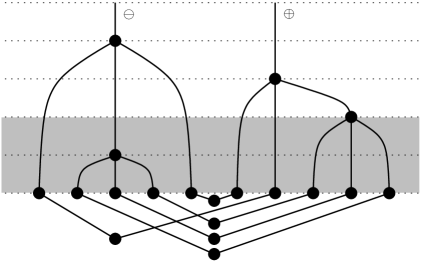
Figure 4: An amputated diagram representing a nonzero $\mathcal{A}_{2}^{\rm ampl}(S,J,\ell,\ell^{\prime},s,\kappa)$ with $\ell^{\prime}=(2,1)$, $\ell=(3,1)$, $J=(+1,-1)$, and using a pairing $S=\{\{1,7\},\{2,10\},\{3,9\},\{4,8\},\{5,6\}\}$. The shading on the first two time slices is used to denote the fact that these time slices have zero length, as explained in the text. As before, the symbols “$\oplus$” and “$\ominus$” denote the roots of the plus and minus trees, respectively.

To complete the above derivation, we still need to prove the time-simplex Lemma.

• Proof of Lemma 4.6  The Lemma is based on rearrangement of the time-integrations by iteratively splitting one of them into two independent parts. The splitting will depend on the relative order of the times accumulated from $s$ and $s^{\prime}$, which is captured by the sum over $J$ on the right hand side. The value of $J_{+}(i;J)$ yields the index for the phase factor $\gamma^{+}$ which is “active” at the new time slice obtained after the splitting. The proof below will be given mainly to show that the above definitions yield a correct description of the result.

  Suppose first that $n=0$. Then the first factor is ${\rm e}^{-{\rm i}t\gamma^{+}_{0}}$. On the other hand, the only admissible $J$ is then $J(i)=-1$ for all $i\in I_{n^{\prime}}$, and thus $J_{+}(i;J)=0$ and $J_{-}(i;J)=i$ for all $i\in I_{0,n^{\prime}}$. Therefore, (4.6) holds by inspection. A symmetrical argument applies to the case $n^{\prime}=0$.

  Assume thus that $n^{\prime}\geq 1$, and we will prove the rest by induction in $n$. The initial case $n=0$ was checked to hold above. Assume then that (4.6) holds for all $n\leq N$, with $N\geq 0$, and consider the case $n=N+1\geq 1$. It is clear that both sides of (4.6) are continuous in $\gamma^{+}_{N+1}$, and thus it suffices to prove it assuming $\gamma^{+}_{N+1}\neq\gamma^{+}_{N}$. Let us first concentrate on the first factor. We change the integration variable from $s_{N}$ to $u=s_{N}+s_{N+1}$. This shows that

  $$\int_{0}^{\infty}\!{\rm d}s_{N}\,\int_{0}^{\infty}\!{\rm d}s_{N+1}\,\delta\Bigl{(}t-\sum_{i=0}^{N+1}s_{i}\Bigr{)}{\rm e}^{-{\rm i}s_{N}\gamma^{+}_{N}-{\rm i}s_{N+1}\gamma^{+}_{N+1}}$$

  $$\quad=\int_{0}^{\infty}\!{\rm d}s_{N+1}\,\int_{s_{N+1}}^{\infty}\!{\rm d}u\,\delta\Bigl{(}t-u-\sum_{i=0}^{N-1}s_{i}\Bigr{)}{\rm e}^{-{\rm i}(u-s_{N+1})\gamma^{+}_{N}-{\rm i}s_{N+1}\gamma^{+}_{N+1}}$$

  $$\quad=\int_{0}^{\infty}\!{\rm d}u\,\delta\Bigl{(}t-u-\sum_{i=0}^{N-1}s_{i}\Bigr{)}{\rm e}^{-{\rm i}u\gamma^{+}_{N}}\int_{0}^{u}\!{\rm d}s_{N+1}\,{\rm e}^{-{\rm i}s_{N+1}(\gamma^{+}_{N+1}-\gamma^{+}_{N})}$$

  $$\quad=\frac{{\rm i}}{\gamma^{+}_{N+1}-\gamma^{+}_{N}}\int_{0}^{\infty}\!{\rm d}u\,\delta\Bigl{(}t-u-\sum_{i=0}^{N-1}s_{i}\Bigr{)}\Bigl{(}{\rm e}^{-{\rm i}u\gamma^{+}_{N+1}}-{\rm e}^{-{\rm i}u\gamma^{+}_{N}}\Bigr{)}.$$ (4.31)

  The induction assumption can be applied to both terms separately, which proves that (4.6) is equal to

  $$\frac{{\rm i}}{\gamma^{+}_{N+1}-\gamma^{+}_{N}}\sum_{J\text{ interlaces }(N,n^{\prime})}\int_{({\mathbb{R}}_{+})^{I_{0,N+n^{\prime}}}}\!{\rm d}r\,\delta\Bigl{(}t-\sum_{i=0}^{N+n^{\prime}}r_{i}\Bigr{)}$$

  $$\qquad\times\Bigl{(}\prod_{i=0}^{N+n^{\prime}}\left.{\rm e}^{-{\rm i}r_{i}(\gamma^{+}_{J_{+}(i;J)}+\gamma^{-}_{J_{-}(i;J)})}\right|_{\gamma^{+}_{N}\to\gamma^{+}_{N+1}}-\prod_{i=0}^{N+n^{\prime}}{\rm e}^{-{\rm i}r_{i}(\gamma^{+}_{J_{+}(i;J)}+\gamma^{-}_{J_{-}(i;J)})}\Bigr{)}.$$ (4.32)

  For a fixed $J$, let $j_{0}=\min\left\{i\in I_{0,N+n^{\prime}}\left|\,J_{+}(i;J)=N\makebox[0.0pt]{$\displaystyle\phantom{i\in I_{0,N+n^{\prime}}}$}\right.\!\right\}$, i.e., $j_{0}$ denotes the last appearance of $+1$ in $J$. Then $N\leq j_{0}\leq N+n^{\prime}$. The difference in the brackets can then be expressed as

  $$\prod_{i=0}^{N+n^{\prime}}{\rm e}^{-{\rm i}r_{i}\gamma^{-}_{J_{-}(i;J)}}\prod_{i=0}^{j_{0}-1}{\rm e}^{-{\rm i}r_{i}\gamma^{+}_{J_{+}(i;J)}}\Bigl{(}{\rm e}^{-{\rm i}\gamma^{+}_{N+1}\sum_{i=j_{0}}^{N+n^{\prime}}r_{i}}-{\rm e}^{-{\rm i}\gamma^{+}_{N}\sum_{i=j_{0}}^{N+n^{\prime}}r_{i}}\Bigr{)}$$

  $$\quad=(-i)(\gamma^{+}_{N+1}-\gamma^{+}_{N})\prod_{i=0}^{N+n^{\prime}}{\rm e}^{-{\rm i}r_{i}\gamma^{-}_{J_{-}(i;J)}}\prod_{i=0}^{j_{0}-1}{\rm e}^{-{\rm i}r_{i}\gamma^{+}_{J_{+}(i;J)}}$$

  $$\qquad\times\left.\int_{0}^{u}\!{\rm d}s\,{\rm e}^{-{\rm i}s\gamma^{+}_{N}}{\rm e}^{-{\rm i}(u-s)\gamma^{+}_{N+1}}\right|_{u=\sum_{i=j_{0}}^{N+n^{\prime}}r_{i}}\,.$$ (4.33)

  Set $S_{\ell}=\sum_{i=j_{0}}^{\ell-1}r_{i}$. The final integral is split according to the position of $s$ in the sequence $(S_{\ell})_{\ell=j_{0},\ldots,N+n^{\prime}+1}$. This yields

  $$\sum_{\ell=j_{0}}^{N+n^{\prime}}\int_{0}^{\infty}\!{\rm d}s\,{\mathbbm{1}}(S_{\ell}\leq s\leq S_{\ell+1}){\rm e}^{-{\rm i}s\gamma^{+}_{N}}{\rm e}^{-{\rm i}(S_{N+n^{\prime}+1}-s)\gamma^{+}_{N+1}}\,.$$ (4.34)

  Given a map $J$ and $\ell\in\{j_{0}(J),N+n^{\prime}\}$, we define a map $J^{\prime}=J^{\prime}_{\ell,J}:I_{N+1+n^{\prime}}\to\{\pm 1\}$ by the rule

  $$J^{\prime}(i)=\begin{cases}J(i),&\text{if }i\leq\ell,\\ +1,&\text{if }i=\ell+1,\\ -1,&\text{if }i>\ell+1.\end{cases}$$ (4.35)

  Obviously, $J^{\prime}$ interlaces $(N+1,n^{\prime})$, and the maps $J_{\pm}(\cdot;J^{\prime})$ then satisfy $J_{\pm}(i;J^{\prime})=J_{\pm}(i;J)$ for $i\leq\ell$ and $J_{+}(i;J^{\prime})=N+1$, $J_{-}(i;J^{\prime})=J_{-}(i-1;J)$ for $i>\ell$. Conversely, if $J^{\prime\prime}$ is an arbitrary map interlacing $(N+1,n^{\prime})$ then there are unique $\ell$ and $J$ such that $J^{\prime\prime}=J^{\prime}_{\ell,J}$, determined by the choices $\ell=j_{0}(J^{\prime\prime})$, and $J$ obtained from $J^{\prime\prime}$ by canceling $\ell$. Therefore,

  $$\sum_{J^{\prime}\text{ interlaces }(N+1,n^{\prime})}F(J^{\prime})=\sum_{J\text{ interlaces }(N,n^{\prime})}\sum_{\ell=j_{0}(J)}^{N+n^{\prime}}F(J^{\prime}_{\ell,J})\,.$$ (4.36)

Thus we only need to prove that the remaining integrals are equal, i.e., that the integral on the right hand side of (4.6) for $J\to J^{\prime}=J^{\prime}_{\ell,J}$ and $n\to N+1$, is equal to

$$\int_{({\mathbb{R}}_{+})^{I_{0,N+n^{\prime}}}}\!{\rm d}r\,\delta\Bigl{(}t-\sum_{i=0}^{N+n^{\prime}}r_{i}\Bigr{)}\prod_{i=0}^{N+n^{\prime}}{\rm e}^{-{\rm i}r_{i}\gamma^{-}_{J_{-}(i;J)}}\prod_{i=0}^{j_{0}-1}{\rm e}^{-{\rm i}r_{i}\gamma^{+}_{J_{+}(i;J)}}$$

$$\quad\times\int_{0}^{\infty}\!{\rm d}s\,{\mathbbm{1}}(S_{\ell}\leq s\leq S_{\ell+1}){\rm e}^{-{\rm i}s\gamma^{+}_{N}}{\rm e}^{-{\rm i}(S_{N+n^{\prime}+1}-s)\gamma^{+}_{N+1}}\,.$$ (4.37)

To see this, let us change the integration variables $(r_{i},s)_{i}$ to $(r^{\prime}_{j})_{j}$ by using $r^{\prime}_{j}=r_{j}$ for $j<\ell$, $r^{\prime}_{j}=r_{j-1}$ for $\ell<j\leq N+1+n^{\prime}$, and $r^{\prime}_{\ell}=s-S_{\ell}$, $r^{\prime}_{\ell+1}=S_{\ell}+r_{\ell}-s$. Since $S_{\ell}$ does not depend on $r_{\ell}$, the Jacobian can straightforwardly be checked to be equal to one, and the effect of ${\mathbbm{1}}(S_{\ell}\leq s\leq S_{\ell+1})$ is simply to restrict the integration region to $r^{\prime}\in({\mathbb{R}}_{+})^{I_{0,N+1+n^{\prime}}}$. On the other hand, $r_{\ell}=r^{\prime}_{\ell}+r^{\prime}_{\ell+1}$ and thus

$$\sum_{i=0}^{N+n^{\prime}}r_{i}\gamma^{-}_{J_{-}(i;J)}=\sum_{i=0}^{N+1+n^{\prime}}r^{\prime}_{i}\gamma^{-}_{J_{-}(i;J^{\prime})}$$ (4.38)

and, as $s=\sum_{i=j_{0}}^{\ell}r^{\prime}_{i}$, then also

$$s\gamma^{+}_{N}+(S_{N+n^{\prime}+1}-s)\gamma^{+}_{N+1}=\sum_{i=j_{0}}^{\ell}r^{\prime}_{i}\gamma^{+}_{N}+\sum_{i=\ell+1}^{N+1+n^{\prime}}r^{\prime}_{i}\gamma^{+}_{N+1}=\sum_{i=j_{0}}^{N+1+n^{\prime}}r^{\prime}_{i}\gamma^{+}_{J_{+}(i;J^{\prime})}\,.$$ (4.39)

Thus relabeling of the integration variables now proves that (4.3) is equal to the integral on the right hand side of (4.6). This finishes the proof of the Lemma.∎

5 Resolution of the momentum constraints

One important element for our estimates is disentangling the complicated momentum dependencies into more manageable form which allows iteration of a finite collection of bounds. For this we have to carefully assign which of the momenta are freely integrated over, and which are used to integrate out the $\delta$-functions and thus attain a linear dependence on the free integration variables. We begin from a diagram as described in the previous section, which can represent either a main term or an amputated amplitude. To make full use of graph invariants, we then add one more $\delta$-function to the integrand: we multiply it by a factor

$$1=\int_{\Lambda^{*}}\!{\rm d}k_{e_{0}}\,\delta_{\Lambda}(k_{e_{0}}-k-k^{\prime})\,,$$ (5.1)

where $k$ is the outgoing momentum at the root of the plus tree, and $k^{\prime}$ at the root of the minus tree. (Using the notations of the previous section, we thus have $k=k_{n,1}$, $k^{\prime}=k_{0,0}$ for a main term, and $k=k_{n,1}$, $k^{\prime}=k^{\prime}_{n,1}$ for an amputated term.) The factor will facilitate the analysis of the momentum constraints, as without it there would be one free integration variable which is not associated with a loop in the corresponding graph. This would lead to unnecessary repetition in the oncoming proofs in form of spurious “special cases”, which can now be avoided at the cost of introducing a “spurious edge” into the graph. The additional $\delta$-function can then be accounted for by introducing two additional vertices and one extra edge to the graph: one “fusion vertex” which connects the two edges related to $k$ and $k^{\prime}$, and one vertex to the top of the graph, so that $e_{0}$ is the edge connecting the two new vertices. (See Fig. 5 for an illustration.)

Figure 5: An example of a momentum graph $\mathcal{G}$ constructed by the algorithm described in Section 5. The vertices of the graph are denoted by “bullets”, connected by the edges, the bending of which serves only an illustrative purpose. The graph corresponds to a case with $n=3$, $n^{\prime}=2$ interactions, and a cluster decomposition $S=\{\{1,2\},\{3,4,7\},\{5,6,9,12\},\{8,10,11\}\}$, using an enumeration of the vertices in $\mathcal{V}_{\rm 0}$ from left to right in the figure. Examples of the notations used for the different vertices are also given, in particular, we have denoted the division of the vertices into the four disjoint sets on the right. The horizontal dotted lines divide the graph into the time slices, and the labels on the left show some values of the function $\tau$. Finally, the signs near the vertices on the bottom left half of the graph denote how the edges at the vertex are divided between the sets $\mathcal{E}_{\pm}(v)$.

The diagram obtained this way is called the momentum graph associated with the original amplitude, and it consist of $\mathcal{G}=(\mathcal{V},\mathcal{E})$, where $\mathcal{V}$ collects the vertices and $\mathcal{E}$ the edges of the graph. There is also additional structure arising from the construction of the graph and related to the different roles the vertices play. In particular, the fusion vertices have a natural time-ordering determined by $\ell$, $\ell^{\prime}$ and $J$, and encoded in the way we have drawn the diagrams.

Let us first summarize the construction of the momentum graph, and introduce related notation for later use. The total time $t$ and the partial time-integration variables $\kappa_{i}$ are parameters which do not affect the momentum structure, and we assume them to be fixed to some allowed value in the following. The amplitude depends on $S$, the cluster partitioning of the initial fields, and the number of interactions in the plus and minus trees, $n$ and $n^{\prime}$, as well as the related collisions histories determined by $\ell$, $\ell^{\prime}$ and $J$. (For a main term graph $n^{\prime}=0$, and $\ell^{\prime}$ and $J$ are then not relevant.) We let $N=n+n^{\prime}$ denote the total number of interactions, and consider here only the non-trivial case $N\geq 1$. Given these parameters, we can construct the momentum graph $\mathcal{G}$ by the following iteration procedure.

At each iteration step, for the given previous graph $\mathcal{G}=(\mathcal{V},\mathcal{E})$ with $\mathcal{V}\neq\emptyset$ we construct a new graph $\mathcal{G}^{\prime}=(\mathcal{V}^{\prime},\mathcal{E}^{\prime})$ by either “attaching a new edge” to some given $v\in\mathcal{V}$, or by “joining the vertices” $v,v^{\prime}\in\mathcal{V}$, $v^{\prime}\neq v$. Explicitly, in the first case when a new edge is attached to $v\in\mathcal{V}$, we choose a new vertex label $u\not\in\mathcal{V}$, and define $\mathcal{V}^{\prime}=\mathcal{V}\cup\{u\}$ and $\mathcal{E}^{\prime}=\mathcal{E}\cup\{\{v,u\}\}$. In our iteration scheme, the new vertex label $u$ will be a dummy variable, which we can choose to relabel later. In the second case, when two existing vertices $v,v^{\prime}$ are joined, we define $\mathcal{V}^{\prime}=\mathcal{V}$ and $\mathcal{E}^{\prime}=\mathcal{E}\cup\{\{v,v^{\prime}\}\}$. The iterative construction will thus imply a natural order for the edges of the graph: we will say in the following that $e<f$ if the edge $e$ is created before $f$. This defines then a complete order $e\leq f$ on $\mathcal{E}$. We will use the creation order also to label the edges: $e_{i}$ is the edge which is created in the $i$:th iteration step.

We begin with $\mathcal{G}^{(0)}=(\mathcal{V}^{(0)},\mathcal{E}^{(0)})$ where $\mathcal{V}^{(0)}=\{v_{\rm R},v_{N+1}\}$ and $\mathcal{E}^{(0)}=\{e_{0}\}$, $e_{0}=\{v_{\rm R},v_{N+1}\}$. We next go through the list $i=1,2,\ldots,N_{k}$, where $N_{k}$ is the total number of $k,k^{\prime}$-integrals. At each iteration step, we add the corresponding edge to $\mathcal{E}$. In the first two iteration steps we attach two new edges, labeled $e_{1}$ and $e_{2}$, to $v_{N+1}$. The edge $e_{1}$ begins the minus tree associated with the $k^{\prime}$-integrals, and the edge $e_{2}$ begins the plus tree associated with the $k$-integrals. If the last interaction (as determined by $J$) is in the minus tree we next choose $e_{1}$, and otherwise choose $e_{2}$, and relabel the unlabeled vertex in it by $v_{N}$.

The next three iteration steps are to attach three new edges to $v_{N}$, left to right in the picture (and thus having parities $-1$, $\sigma$, $1$). The interaction history is determined by $\ell,\ell^{\prime},J$, and is used (backwards in time) for choosing a unique edge with an unlabeled vertex in the following steps. We pick the appropriate edge and label the (unique) unlabeled vertex in this edge as $v_{N-1}$, and the next three iteration steps consist of attaching three new edges to $v_{N-1}$, left to right. This procedure of attaching triplets of edges is iterated altogether $N$ times and results in a tree starting from $v_{\rm R}$.

The resulting vertex set is composed of $N+2$ labeled and of $2N+2$ unlabeled vertices. The labeled vertices belong either to $\mathcal{V}_{\rm R}=\{v_{\rm R}\}$ or to $\mathcal{V}_{\rm F}=\{v_{j}\}_{j=1,\ldots,N+1}$, which we call the root and the fusion vertex set, respectively. The term interaction vertex refers to an interaction vertex in the original diagram. The set of interaction vertices is thus $\mathcal{V}_{\rm I}=\mathcal{V}_{\rm F}\setminus\{v_{N+1}\}$. We collect the remaining vertices to $\mathcal{V}_{\rm 0}$, and call this the initial time vertex set. Each $v\in\mathcal{V}_{\rm 0}$ is associated with a definite $\psi$-factor in the initial time expectation value, and $S$ can thus be identified with a unique partition of $\mathcal{V}_{\rm 0}$ into clusters. For every cluster $A$ in $S$, we associate an independent label $u_{A}$. The set $\mathcal{V}_{\rm C}=\{u_{A}\}_{A\in S}$ is called the cluster vertex set. The final graph $\mathcal{G}$ is defined to have a vertex set $\mathcal{V}=\mathcal{V}_{\rm R}\cup\mathcal{V}_{\rm F}\cup\mathcal{V}_{\rm 0}\cup\mathcal{V}_{\rm C}$. In the final iteration steps, we add edges by going through the initial time vertices, left to right, and for each vertex $v$ joining it to $u_{A(v)}$ where $A(v)\in S$ is the unique cluster containing $v$.

This yields an unoriented graph $\mathcal{G}=\mathcal{G}(S,J,n,\ell,n^{\prime},\ell^{\prime})=(\mathcal{V},\mathcal{E})$ representing the corresponding amplitude. The vertices have a natural time-order given by $\tau:\mathcal{V}\to[0,N+2]$, which we define by setting for $v\in\mathcal{V}$

$$\tau(v)=\begin{cases}N+2,&\text{if }v\in\mathcal{V}_{\rm R},\\ j,&\text{if there is }j\in\{1,\ldots,N+1\}\text{ such that }v=v_{j},\\ 0,&\text{if }v\in\mathcal{V}_{\rm 0}\cup\mathcal{V}_{\rm C}.\end{cases}$$ (5.2)

We extend the time-ordering to the edges by defining $\hat{\tau}(e)=\max\left\{\tau(v)\left|\,v\in e\makebox[0.0pt]{$\displaystyle\phantom{\tau(v)}$}\right.\!\right\}$ for $e\in\mathcal{E}$. It is obvious from our construction that $e\leq f$ implies $\hat{\tau}(e)\geq\hat{\tau}(f)$.

For any $v\in\mathcal{V}$, let $\mathcal{E}(v)=\left\{e\in\mathcal{E}\left|\,v\in e\makebox[0.0pt]{$\displaystyle\phantom{e\in\mathcal{E}}$}\right.\!\right\}$ denote the set of edges attached to $v$. To each edge $e\in\mathcal{E}$ we have associated an integration over a variable $k_{e}$. These variables are not independent since, apart from the root vertex, each vertex has a $\delta$-function associated to it. Explicitly, for $v\not\in\mathcal{V}_{\rm R}$, there is a factor (Kirchhoff rule)

$$\delta_{\Lambda}\Big{(}\sum_{e\in\mathcal{E}_{+}(v)}k_{e}-\sum_{e\in\mathcal{E}_{-}(v)}k_{e}\Big{)},$$ (5.3)

with $\mathcal{E}(v)=\mathcal{E}_{+}(v)\cup\mathcal{E}_{-}(v)$. How the edges are split between the two sets depends on the type of vertex. If $v\in\mathcal{V}_{\rm C}$, then $\mathcal{E}_{-}=\emptyset$ and $\mathcal{E}_{+}=\mathcal{E}(v)$. Otherwise, $\mathcal{E}_{+}(v)=\{e\}$, where $e$ is the first edge attached to $v$, and $\mathcal{E}_{-}(v)=\mathcal{E}(v)\setminus\{e\}\neq\emptyset$. We have illustrated these definitions in the example graph in Fig. 5 (The graph has $n^{\prime},n>0$ with $n^{\prime}\neq n$, and as such is not related to any of the present amplitudes. However, we use the more general graph to show that the scheme does not depend on the special relation between $n$ and $n^{\prime}$.)

Our aim is next to “integrate out” all the constraint $\delta$-functions. We do this by associating with every vertex a unique edge attached to it which we use for the integration. As long as we use each edge not more than once, this results in a complete resolution of the momentum constraints. The edges used in the integration of the $\delta$-functions are called integrated, and the remaining edges are called free. We use the notation $\mathcal{E}^{\prime}$ for the collection of integrated edges and $\mathcal{F}$ for the free edges. The following theorem shows that there is a way of achieving such a division of edges which respects their natural time-ordering.

Theorem 5.1

Consider a momentum graph $\mathcal{G}$. There exists a complete integration of the momentum constraints, determined by a certain unique spanning tree of the graph, such that for any free edge $f$ all $k_{e}$ with $e<f$ are independent of $k_{f}$. In addition, all free edges end at a fusion vertex: if $f$ is free, there is a fusion vertex $v\in\mathcal{V}_{\rm F}$ and $v^{\prime}\in\mathcal{V}$ such that $\tau(v)>\tau(v^{\prime})$ and $f=\{v,v^{\prime}\}$.

From now on, we assume that the momentum constraints are integrated out using the unique construction in Theorem 5.1. For any fusion vertex $v\in\mathcal{V}_{\rm F}$, we call the number of free edges in $\mathcal{E}_{-}(v)$ the degree of the fusion vertex, and denote this by $\deg v$. The following theorem summarizes how the integrated edges ending at an interaction vertex depend on its free momenta.

Proposition 5.2

The degree of a fusion vertex belongs to $\{0,1,2\}$. If $v\in\mathcal{V}_{\rm I}$ is a degree one interaction vertex, then $\mathcal{E}_{-}(v)=\{f,e,e^{\prime}\}$ where $f$ is a free edge, and $k_{e}=-k_{f}+G$, $k_{e^{\prime}}=G^{\prime}$, where $G$ and $G^{\prime}$ are independent of $k_{f}$. If $v$ is a degree two interaction vertex, then $\mathcal{E}_{-}(v)=\{f,f^{\prime},e\}$ where $f,f^{\prime}$ are free edges, and $k_{e}=-k_{f}-k_{f^{\prime}}+G$, where $G$ is independent of $k_{f}$ and $k_{f^{\prime}}$.

We will need other similar properties of the integrated momenta, to be given later in this section. However, let us first explain how the constraints are removed.

• Proof of Theorem 5.1 and Proposition 5.2  We construct a spanning tree for $\mathcal{G}$ which provides a recipe for integration of the vertex $\delta$-constraints and leads to the properties stated in Theorem 5.1. We first construct an unoriented tree $\mathcal{T}=(\mathcal{V}_{\mathcal{T}},\mathcal{E}_{\mathcal{T}})$ from $\mathcal{G}$, and then define an oriented tree $\mathcal{T}_{\rm o}=(\mathcal{V}_{\mathcal{T}},\mathcal{E}_{\mathcal{T}_{\rm o}})$ by assigning an orientation to each of the edges in $\mathcal{E}_{\mathcal{T}}$.

  Let $\mathcal{T}^{(0)}=(\mathcal{V}_{\mathcal{T}}^{(0)},\mathcal{E}_{\mathcal{T}}^{(0)})$, with $\mathcal{V}_{\mathcal{T}}^{(0)}=\emptyset=\mathcal{E}_{\mathcal{T}}^{(0)}$. We go through all edges in $\mathcal{E}$ in the opposite order they were created, i.e., decreasing with respect to their order. At the iteration step $l$, let $e$ denote the corresponding edge, and consider the previous graph $\mathcal{T}^{(l-1)}$. If adding the edge $e$ to $\mathcal{T}^{(l-1)}$ would create a loop, we define $\mathcal{T}^{(l)}=\mathcal{T}^{(l-1)}$. Otherwise, we define $\mathcal{T}^{(l)}$ as the graph resulting from this addition, i.e., we define $\mathcal{V}_{\mathcal{T}}^{(l)}=\mathcal{V}_{\mathcal{T}}^{(l-1)}\cup e$, and $\mathcal{E}_{\mathcal{T}}^{(l)}=\mathcal{E}_{\mathcal{T}}^{(l-1)}\cup\{e\}$. Since in the first case necessarily $e\subset\mathcal{V}_{\mathcal{T}}^{\ell-1}$, we will always have $e\subset\mathcal{V}_{\mathcal{T}}^{\ell}$, and thus no vertex in $e$ can be lost in the iteration step.

  Let $\mathcal{T}=(\mathcal{V}_{\mathcal{T}},\mathcal{E}_{\mathcal{T}})$ denote the graph obtained after the final iteration step. By construction, at each step $\mathcal{T}^{(\ell)}$ is a forest, and thus so is $\mathcal{T}$. Moreover, since $\mathcal{G}$ is connected, $\mathcal{T}$ is actually a tree. Since every vertex in $\mathcal{V}$ is contained in some edge, we also have $\mathcal{V}_{\mathcal{T}}=\mathcal{V}$. In addition, $\mathcal{E}_{\mathcal{T}}\subset\mathcal{E}$, and every $e\in\mathcal{E}\setminus\mathcal{E}_{\mathcal{T}}$ has the following property: adding it to $\mathcal{E}_{\mathcal{T}}$ would make a unique loop composed out of edges $\{e^{\prime}\}$ each of which satisfies $e^{\prime}\geq e$, and thus also $\hat{\tau}(e^{\prime})\leq\hat{\tau}(e)$. (The loop is unique since $\mathcal{T}$ itself has no loops.)

  Next we create $\mathcal{T}_{\rm o}$ by assigning an orientation to the edges of $\mathcal{T}$. We root the tree at $v_{\rm R}$. This is achieved by the following algorithm: we first note that for any vertex $v$ there is a unique path connecting it to $v_{\rm R}$. We orient the edges of the path so that it starts from $v$ and ends in $v_{\rm R}$. This is iterated for all vertices in the tree. Although it is possible that two different vertices share edges along the path, these edges are assigned the same orientation at all steps of the algorithm. (If two such paths share any vertex, then the paths must coincide past this vertex; otherwise there would be a loop in the graph.) This results in an oriented graph in which for every $v\in\mathcal{V}\setminus\mathcal{V}_{\rm R}$ there is a unique edge $E(v)\in\mathcal{E}(v)$ pointing out of the vertex. In addition, the map $E:\mathcal{V}\setminus\mathcal{V}_{\rm R}\to\mathcal{E}$ is one-to-one. Thus we can integrate all the momentum $\delta$-functions, by using the variable $k_{E(v)}$ for the $\delta$-function at the vertex $v\in\mathcal{V}\setminus\mathcal{V}_{\rm R}$. We have depicted the oriented tree resulting from the graph of Fig. 5 in Fig. 6.

  

  Figure 6: The oriented spanning tree $\mathcal{T}_{\rm o}$ corresponding to the graph $\mathcal{G}$ given in Fig. 5. The edges in the complement of the tree have also been depicted by dashed lines. The enumeration $(e_{\ell})$ of the edges corresponds to the one explained in the text; the spanning tree is constructed by adding the edges in the graph in decreasing order.

After the above integration steps, all the constraints have been resolved, and the set of remaining integration variables will consist of $k_{e}$ with $e\in\mathcal{E}\setminus\mathcal{E}_{\mathcal{T}}$. These are all free integration variables, and thus $\mathcal{F}:=\mathcal{E}\setminus\mathcal{E}_{\mathcal{T}}$ is the set of free edges, and $\mathcal{E}^{\prime}:=\mathcal{E}_{\mathcal{T}}$ is the set of integrated edges. Obviously, one has to add at least all edges attached to a cluster vertex before a loop can be created, and thus no such edge is free. Also, the addition of the last edge $e_{0}$ never creates a loop. All remaining edges end at a fusion vertex, and thus this is true also of all free edges.

In order to conclude the proof of Theorem 5.1, we need to find out how the integrated momenta depend on the free ones. For later use, let us spell out also this fairly standard part in detail. For any $v\in\mathcal{V}$, let $\mathcal{F}(v)$ collect the free edges attached to $v$, $\mathcal{F}(v)=\mathcal{E}(v)\cap\mathcal{F}$. Let us also associate for any $v\in\mathcal{V}\setminus\mathcal{V}_{\rm R}$ an “edge parity” mapping $\sigma_{v}:\mathcal{E}(v)\to\{-1,+1\}$ defined by

$$\sigma_{v}(e)=\begin{cases}+1,&\text{if }e\in\mathcal{E}_{+}(v),\\ -1,&\text{if }e\in\mathcal{E}_{-}(v).\end{cases}$$ (5.4)

Lemma 5.3

If $e=\{v,v^{\prime}\}\in\mathcal{E}$ does not intersect $\mathcal{V}_{\rm R}$, then $m(e)=-\sigma_{v}(e)\sigma_{v^{\prime}}(e)=1$.

Proof.

Assume first that $v\in\mathcal{V}_{\rm C}$. Then $\sigma_{v}(e)=1$ and $v^{\prime}\in\mathcal{V}_{\rm 0}$. Since $\mathcal{E}(v^{\prime})$ then contains only two elements, of which $e$ is created later, we have $\sigma_{v^{\prime}}(e)=-1$, and thus $m(e)=1$. Assume then $e\cap\mathcal{V}_{\rm C}=\emptyset$. If $v\in\mathcal{V}_{\rm 0}$, then $v^{\prime}\in\mathcal{V}_{\rm F}$, and thus $e$ is the earlier of the two edges attached to $v$ and $\sigma_{v}(e)=1$. However, then it is one of the three later edges attached to $v^{\prime}$, and thus $\sigma_{v^{\prime}}(e)=-1$. This implies $m(e)=1$. Since $m(e)$ is symmetric under the exchange of $v$ and $v^{\prime}$, we can now assume that $e\cap\mathcal{V}_{\rm C}\cap\mathcal{V}_{\rm 0}=\emptyset$. Then both $v,v^{\prime}\in\mathcal{V}_{\rm F}$ and it follows from the construction that $\sigma_{v}(e)\sigma_{v^{\prime}}(e)=-1$. This proves that for any edge $e$ with $e\cap\mathcal{V}_{\rm R}=\emptyset$, $m(e)=1$. ∎∎

Consider then an integrated variable $k_{e}$, with $e\in\mathcal{E}^{\prime}$. The edge $e$ has been assigned an orientation, say $e=(v_{1},v_{2})$, going from the vertex $v_{1}$ to the vertex $v_{2}$. Let $\mathcal{P}(v)$, $v\in\mathcal{V}$, denote the collection of the vertices $v^{\prime}$ for which there exists a path from $v^{\prime}$ to $v$ in the oriented tree $\mathcal{T}_{\rm o}$. In particular, we include here the trivial case $v^{\prime}=v$. We claim that then

$$k_{e}=\sum_{v\in\mathcal{P}(v_{1})}\sum_{f\in\mathcal{F}(v)}\left(-\sigma_{v_{1}}(e)\sigma_{v}(f)\right)k_{f}.$$ (5.5)

This can be proven by induction in a degree $j$ associated with an oriented edge $e=(v_{1},v_{2})\in\mathcal{E}_{\mathcal{T}_{\rm o}}$: $j$ is defined as the maximum of the number of vertices in an oriented path from any leaf to $v_{1}$ (note that such paths always exist). For $j=1$, $v_{1}$ is itself a leaf, and thus $\mathcal{P}(v_{1})=\{v_{1}\}$ and $\mathcal{F}(v_{1})=\mathcal{E}(v_{1})\setminus\{e\}$. Also $v_{1}\not\in\mathcal{V}_{\rm R}$, since the edge $e_{0}$ is always oriented as $(v_{N+1},v_{\rm R})$. Thus there is a $\delta$-function associated with $v_{1}$, and it enforces

$$\sum_{e^{\prime}\in\mathcal{E}(v_{1})}\sigma_{v_{1}\!}(e^{\prime})k_{e^{\prime}}=0.$$ (5.6)

The designated integration of this $\delta$-function yields, with $v=v_{1}$,

$$k_{e}=-\sigma_{v}(e)\sum_{e^{\prime}\in\mathcal{E}(v)\setminus\{e\}}\sigma_{v}(e^{\prime})k_{e^{\prime}}=\sum_{e^{\prime}\in\mathcal{F}(v)}(-\sigma_{v}(e)\sigma_{v}(e^{\prime}))k_{e^{\prime}},$$ (5.7)

and therefore (5.5) holds for $j=1$. Assume then that (5.5) holds for any edge up to degree $j\geq 1$, and suppose $e=(v_{1},v_{2})$ is an edge with a degree $j+1$. Again $v_{1}\not\in\mathcal{V}_{\rm R}$, and the corresponding $\delta$-function implies that, with $v=v_{1}$,

$$k_{e}=\sum_{e^{\prime}\in\mathcal{E}(v)\setminus\{e\}}(-\sigma_{v}(e)\sigma_{v}(e^{\prime}))k_{e^{\prime}}.$$ (5.8)

In the sum, an edge $e^{\prime}$ is either free or it must have a degree of at most $j$, as otherwise $e$ would have a degree of at least $j+2$. Thus by the induction assumption,

$$k_{e}=\sum_{f\in\mathcal{F}(v)}(-\sigma_{v}(e)\sigma_{v}(f))k_{f}+\sum_{e^{\prime}\in\mathcal{E}(v)\setminus\{e\}\setminus\mathcal{F}(v)}(-\sigma_{v}(e)\sigma_{v}(e^{\prime}))$$

$$\qquad\times\sum_{v^{\prime}\in\mathcal{P}(V_{1}(e^{\prime}))}\sum_{f\in\mathcal{F}(v^{\prime})}\left(-\sigma_{V_{1}(e^{\prime})}(e^{\prime})\sigma_{v^{\prime}}(f)\right)k_{f},$$ (5.9)

where $e^{\prime}=(V_{1}(e^{\prime}),v)$ and $V_{1}(e)$ denotes the first vertex of an oriented edge $e$. Therefore,

$$(-\sigma_{v}(e)\sigma_{v}(e^{\prime}))\left(-\sigma_{V_{1}(e^{\prime})}(e^{\prime})\sigma_{v^{\prime}}(f)\right)=-\sigma_{v}(e)m(e^{\prime})\sigma_{v^{\prime}}(f)=-\sigma_{v}(e)\sigma_{v^{\prime}}(f)\,.$$ (5.10)

Now (5) can be checked to coincide with (5.5). This completes the induction step, and thus proves (5.5).

Consider then a free integration variable corresponding to $f_{0}=\{u,u^{\prime}\}\in\mathcal{F}$, where we can choose $\tau(u)>\tau(u^{\prime})$. Then $f_{0}\cap\mathcal{V}_{\rm R}=\emptyset$, $\hat{\tau}(f_{0})=\tau(u)$, and $\sigma_{u}(f_{0})=-1$, $\sigma_{u^{\prime}}(f_{0})=+1$. The unique oriented paths from $u$ and $u^{\prime}$ to the root of the tree must coincide starting from a unique vertex $v_{0}$, which can a priori also be either $u$ or $u^{\prime}$. In addition, the paths before $v_{0}$ cannot have any common vertices. Suppose $e=(v_{1},v_{2})$ belongs to the path from $u$ to $v_{0}$ in $\mathcal{T}_{\rm o}$. Then $k_{e}$ depends on $k_{f_{0}}$, and using (5.5) we find that $k_{e}=\sigma_{v_{1}}(e)k_{f_{0}}+\cdots$. Similarly, if $e$ belongs to the path from $u^{\prime}$ to $v_{0}$, then $k_{e}=-\sigma_{v_{1}}(e)k_{f_{0}}+\cdots$. For any $e$ which comes after $v_{0}$ in the path, both terms will be present, and they cancel each other. Resorting to (5.5) thus proves that only those $k_{e}$ whose edges are contained in either of the paths $u\to v_{0}$ and $u^{\prime}\to v_{0}$ depend on the free variable $k_{f_{0}}$. However, as these edges, together with $f_{0}$, would form a loop in $\mathcal{G}$, it follows from the construction of $\mathcal{T}$ that for any such edge $e$ we have $e\geq f_{0}$. This proves that if $f\in\mathcal{F}$ and $e\in\mathcal{E}$ with $e<f$, $k_{e}$ is either free (and thus independent of $k_{f}$) or by the above result does not depend on $k_{f}$. This completes the proof of Theorem 5.1.

Proposition 5.2 is now a corollary of the above results. The degree of the top fusion vertex is obviously less than two, and since for any vertex adding its first edge cannot create a loop, also the degree of all interaction vertices is less than or equal to two. To prove the second claim, let us assume $u$ is an interaction vertex and consider the three edges belonging to $\mathcal{E}_{-}(u)$, one of which is $f_{0}$. If $v_{0}\neq u$, then there is a non-trivial path from $u$ to $v_{0}$, and we can assume that $e=(u,v_{2})$ is the first edge along this path. Since then $e>f_{0}$, we have $e\in\mathcal{E}_{-}(u)$,and thus $k_{e}=-k_{f_{0}}+\cdots$. If $v_{0}=u$, there is a non-trivial path from $u^{\prime}$ to $u$, and let $e=(v_{1},u)$ be the last edge in that path. By $e>f_{0}$, again we then have $e\in\mathcal{E}_{-}(u)$. Since $m(e)=1$, we find $k_{e}=-\sigma_{v_{1}}(e)k_{f_{0}}+\cdots=\sigma_{u}(e)k_{f_{0}}+\cdots=-k_{f_{0}}+\cdots$. Finally, consider the third edge $e^{\prime}\in\mathcal{E}_{-}(u)$. This cannot belong to either of the paths from $u\to v_{0}$ and $u^{\prime}\to v_{0}$, and thus $k_{e^{\prime}}$ is always independent of $k_{f_{0}}$. If $e^{\prime}$ is integrated, the degree of $u$ is one, and we have proved the statement made in the Proposition. If $e^{\prime}$ is a free edge, the degree of $u$ is two. If we then apply the above result to $e^{\prime}$ instead of $f_{0}$, we can conclude that $k_{e}=-k_{e^{\prime}}-k_{f_{0}}+\cdots$, where the remainder is independent of both $k_{e^{\prime}}$ and $k_{f_{0}}$. (Note that $e$ is then the only integrated edge in $\mathcal{E}_{-}(u)$, and must therefore contain both of the free variables.) This completes also the proof of Proposition 5.2.∎

In the following, the term oriented path refers to a path in $\mathcal{T}_{\rm o}$. Without this clarifier, a path always refers to an unoriented path in a subgraph of $\mathcal{G}$. The following Lemma improves on (5.5) and yields the exact dependence of integrated momenta on the free ones.

Lemma 5.4

For any integrated edge $e=(v_{1},v_{2})\in\mathcal{E}^{\prime}$, let $P=\mathcal{P}(v_{1})$ denote the collection of vertices such that there is an oriented path from the vertex to $v_{1}$. Then

$$k_{e}=\sum_{v\in P}\sum_{f=\{v,v_{f}\}\in\mathcal{F}(v)}{\mathbbm{1}}(v_{f}\not\in P)\left(-\sigma_{v_{1}}(e)\sigma_{v}(f)\right)k_{f}.$$

$$\quad=-\sigma_{v_{1}}(e)\sum_{f\in\mathcal{F}}{\mathbbm{1}}(\exists v\in f\cap P\text{ and }f\cap P^{c}\neq\emptyset)\sigma_{v}(f)k_{f}.$$ (5.11)

In addition, any $f=\{v,v^{\prime}\}\in\mathcal{E}$, such that $f\neq e$, $v\in P$, and $v^{\prime}\not\in P$, is free.

Proof.

By (5.5) the result in (5.4) holds without the characteristic function ${\mathbbm{1}}(v_{f}\not\in\mathcal{P}(v_{1}))$. Consider thus $v,v^{\prime}\in\mathcal{P}(v_{1})$, $v^{\prime}\neq v$, such that $f=\{v,v^{\prime}\}$ is free. Then $\sigma_{v}(f)=-\sigma_{v^{\prime}}(f)$, and thus $-\sigma_{v_{1}}(e)\sigma_{v}(f)-\sigma_{v_{1}}(e)\sigma_{v^{\prime}}(f)=0$. Now sums over edges in $\mathcal{F}(v)$ and $\mathcal{F}(v^{\prime})$ appear in (5.5), and thus the terms proportional to $k_{f}$ in these sums cancel each other. This proves (5.4).

To prove the last statement let us assume the converse. We suppose $f$ is not free, which implies that $f$ has a representative in $\mathcal{T}_{\rm o}$. Suppose first that it is $(v,v^{\prime})$. There is a unique oriented path from $v^{\prime}$ to the root of the corresponding oriented tree. Since $v^{\prime}\not\in P$, the path does not contain $v_{1}$. This however is not possible because there is also an oriented path from $v$ to $v_{1}$ to the root (otherwise $\mathcal{T}$ contains a loop).

Therefore, we only need to consider $f=(v^{\prime},v)$. Then there is an oriented path from $v$ to $v_{1}$, and thus also an oriented path from $v^{\prime}$ to $v_{1}$. This contradicts $v^{\prime}\not\in P$, and thus we can conclude that $f$ must be free. ∎∎

Corollary 5.5

For any edge $e\in\mathcal{E}$, there is a unique collection of free edges $\mathcal{F}_{e}$, and of $\sigma_{e,f}\in\{\pm 1\}$, $f\in\mathcal{F}_{e}$, such that

$$k_{e}=\sum_{f\in\mathcal{F}_{e}}\sigma_{e,f}k_{f}\,.$$ (5.12)

In addition, $k_{e}$ is independent of all free momenta if and only if $k_{e}=0$. This is equivalent to $\mathcal{F}_{e}=\emptyset$, which occurs if and only if the number of connected components increases by one when the edge $e$ is removed from $\mathcal{G}$.

Proof.

If $e\in\mathcal{F}$, we choose $\mathcal{F}_{e}=\{e\}$ and $\sigma_{e,e}=1$. Otherwise, the existence part follows from the Lemma. Suppose there are two such expansions given by $\mathcal{F}_{e}$, $\sigma_{\cdot,e}$ and $\mathcal{F}^{\prime}_{e}$, $\sigma^{\prime}_{\cdot,e}$. If $\mathcal{F}^{\prime}_{e}\neq\mathcal{F}_{e}$, the difference of the expansions would contain some free momenta with coefficients $\pm 1$, and if $\mathcal{F}^{\prime}_{e}=\mathcal{F}_{e}$ but $\sigma^{\prime}_{\cdot,e}\neq\sigma_{\cdot,e}$, some free momenta would appear in the difference with coefficients $\pm 2$. This proves that the expansion is unique.

Obviously, $k_{e}$ is a constant if and only if $\mathcal{F}_{e}=\emptyset$, when $k_{e}=0$. If $e$ is free, then $\mathcal{F}_{e}$ is not empty. Since the spanning tree is then not affected by removal of $e$, the number of connected components remains unchanged by the removal. Therefore, the Corollary holds in this case.

Else $e=(v_{1},v_{2})$ is an integrated edge and we can apply Lemma 5.4. Denote $P=\mathcal{P}(v_{1})$, and suppose there is a path from $v_{1}$ to $v_{2}$ which does not contain $e$. In this case, removing $e$ from $\mathcal{G}$ does not create any new components. Along this path there is an edge $f=\{v,v^{\prime}\}$ such that $v\in P$ but $v^{\prime}\not\in P$. Since $f\neq e$, by Lemma 5.5, $f\in\mathcal{F}$. This implies that $k_{e}$ depends on $k_{f}$, and is not uniformly zero, in accordance with the Corollary.

Finally, assume that every path from $v_{1}$ to $v_{2}$ contains $e$. This implies that $v_{1}$ and $v_{2}$ belong to different components if $e$ is removed from $\mathcal{G}$. However, then there still must be a path from any vertex to either $v_{1}$ or $v_{2}$, and the number of components is thus exactly two. Suppose $f=\{v,v^{\prime}\}\in\mathcal{F}_{e}$, and choose $v\in P$, $v^{\prime}\not\in P$. Following the oriented paths in the opposite direction, we obtain paths $v_{1}\to v$, $v_{\rm R}\to v_{2}$ which do not contain $e$. Since the oriented path $v^{\prime}\to v_{\rm R}$ does not contain $e$, we can join the three segments with $f$ into a path $v_{1}\to v_{2}$ which avoids $e$. This contradicts the assumption, and thus now $\mathcal{F}_{e}=\emptyset$. This completes the proof of the Corollary. ∎∎

Since removing $e_{0}$ from $\mathcal{G}$ isolates $v_{\rm R}$, the Corollary implies that always $k_{e_{0}}=0$, i.e., the sum of the top momenta of plus and minus trees is zero. We have already used this property in the derivation of the amplitudes.

Lemma 5.6

Suppose $f,f^{\prime}$ are the two free edges ending at a degree two interaction vertex $v_{0}\in\mathcal{V}_{\rm I}$. Let $e=(v_{1},v_{2})\in\mathcal{E}^{\prime}$ be an integrated edge. Then $k_{e}=F_{e}(k_{f},k_{f^{\prime}})+G_{e}$ where $G_{e}$ is independent of $k_{f},k_{f^{\prime}}$ and $(k,k^{\prime})\mapsto F_{e}(k,k^{\prime})$ is one of the following seven functions: $0$, $\pm k$, $\pm k^{\prime}$, $\pm(k+k^{\prime})$.

Let $v\in\mathcal{V}_{\rm I}$, and suppose $e,e^{\prime}\in\mathcal{E}_{-}(v)$, $e\neq e^{\prime}$. Then $k_{e}+k_{e^{\prime}}=F(k_{f},k_{f^{\prime}})+G$ where $G$ is independent of $k_{f},k_{f^{\prime}}$ and $(k,k^{\prime})\mapsto F(k,k^{\prime})$ is also one of the above seven functions. If $v=v_{0}$, the choice is reduced to one of the functions $-k$, $-k^{\prime}$, and $k+k^{\prime}$.

Proof.

There are $w,w^{\prime}\in\mathcal{V}_{\rm I}\cup\mathcal{V}_{\rm C}$ such that $k_{f}=\{v,w\}$, $k_{f^{\prime}}=\{v,w^{\prime}\}$. Then $\sigma_{w}(f)=1=\sigma_{w^{\prime}}(f^{\prime})$ and $\sigma_{v}(f)=-1=\sigma_{v}(f^{\prime})$. We express $k_{e}$ using (5.5), which shows that $k_{e}=F_{e}+G_{e}$ where $F_{e}=-\sigma_{v_{1}}(e)(-o_{v}(k_{f}+k_{f^{\prime}})+o_{w}k_{f}+o_{w^{\prime}}k_{f^{\prime}})$, and $o_{x}$ is one, if there is an oriented path from the vertex $x$ to $v_{1}$, and zero otherwise. Checking all combinations produces the list of seven functions stated in the Lemma.

Let us then consider the second statement. If $v=v_{0}$, then either $e$ or $e^{\prime}$ is the unique integrated edge in $\mathcal{E}_{-}(v)$, or $e,e^{\prime}$ are equal to the free momenta $f,f^{\prime}$. In the first case, we can apply Proposition 5.2 which shows that either $F=-k$ or $F=-k^{\prime}$ will work, and in the second case we can choose $F=k+k^{\prime}$. We can thus assume $v\neq v_{0}$. If both $e,e^{\prime}$ are free, then $F=0$ works. If only one of the edges is free, then the previous result implies the existence of the decomposition.

Thus we can assume that both edges are integrated, and $e=\{v,w_{1}\}$, $e^{\prime}=\{v,w^{\prime}_{1}\}$, where $w_{1}\neq w^{\prime}_{1}$. Suppose first that $e$ points out from $v$, i.e., $e=(v,w_{1})$. Then $e^{\prime}$ points in, $e^{\prime}=(w^{\prime}_{1},v)$, and any oriented path to $w^{\prime}_{1}$ extends into an oriented path to $v$. Since $\sigma_{w^{\prime}_{1}}(e^{\prime})=1$ and $\sigma_{v}(e)=-1$, we have $k_{e}+k_{e^{\prime}}=F_{e}+F_{e^{\prime}}+G_{e}+G_{e^{\prime}}$ with $F_{e}+F_{e^{\prime}}=-(-o_{v}(k_{f}+k_{f^{\prime}})+o_{w}k_{f}+o_{w^{\prime}}k_{f^{\prime}})-o_{v}(k_{f}+k_{f^{\prime}})+o_{w}k_{f}+o_{w^{\prime}}k_{f^{\prime}}-o^{\prime}_{v}(k_{f}+k_{f^{\prime}})+o^{\prime}_{w}k_{f}+o^{\prime}_{w^{\prime}}k_{f^{\prime}}$, where $o_{x}$ is one, if there is an oriented path from $x$ to $w^{\prime}_{1}$, and $o^{\prime}_{x}$ is one if there is an oriented path from $x$ to $v$ which does not go via $w^{\prime}_{1}$. Thus $F_{e}+F_{e^{\prime}}=-o^{\prime}_{v}(k_{f}+k_{f^{\prime}})+o^{\prime}_{w}k_{f}+o^{\prime}_{w^{\prime}}k_{f^{\prime}}$ is also of the stated form.

In the remaining case, we can assume that both $e$ and $e^{\prime}$ point into $v$: $e=(w_{1},v)$, $e^{\prime}=(w^{\prime}_{1},v)$. If there is an oriented path from a vertex $x$ to $w_{1}$, there cannot be an oriented path from $x$ to $w^{\prime}_{1}$, and vice versa. Since, in addition, $\sigma_{w^{\prime}_{1}}(e^{\prime})=1=\sigma_{w_{1}}(e)$, we have $k_{e}+k_{e^{\prime}}=F_{e}+F_{e^{\prime}}+G_{e}+G_{e^{\prime}}$ with $F_{e}+F_{e^{\prime}}=-(-o_{v}(k_{f}+k_{f^{\prime}})+o_{w}k_{f}+o_{w^{\prime}}k_{f^{\prime}})$ where $o_{x}$ is one if there is an oriented path from $x$ to either $w_{1}$ or $w^{\prime}_{1}$, and zero otherwise. This completes the proof of the Lemma. ∎∎

Proposition 5.7

Suppose $e,e^{\prime}\in\mathcal{E}$, $e\neq e^{\prime}$, are such that $\mathcal{F}_{e}=\mathcal{F}_{e^{\prime}}$. Then either $k_{e}=0=k_{e^{\prime}}$ or removal of $e$ and $e^{\prime}$ from $\mathcal{G}$ splits it into exactly two components.

Proof.

If $\mathcal{F}_{e}=\mathcal{F}_{e^{\prime}}=\emptyset$, then by Corollary 5.5 $k_{e}=0=k_{e^{\prime}}$, and the first alternative holds. If both $e$ and $e^{\prime}$ are free, then $\mathcal{F}_{e}=\mathcal{F}_{e^{\prime}}$ implies $e^{\prime}=e$, which was not allowed. We can thus assume that $k_{e},k_{e^{\prime}}\neq 0$, and that at least one of $e,e^{\prime}$ is integrated. Let $\mathcal{G}^{\prime\prime}$ denote the graph obtained by removing $e$ and $e^{\prime}$ from $\mathcal{G}$.

Suppose first that one edge is free, but the other is not. By symmetry, we can choose $e^{\prime}$ to be the free one, and assume $e=(v_{1},v_{2})$. Let $P=\mathcal{P}(v_{1})$. Since $\mathcal{F}_{e}=\mathcal{F}_{e^{\prime}}=\{e^{\prime}\}$, there are $v\in P$ and $v^{\prime}\not\in P$ such that $e^{\prime}=\{v,v^{\prime}\}$. Removal of $e^{\prime}$ does not change the number of components, since the spanning tree is not affected by it. We thus need to show that the subsequent removal of $e$ will split the component. Suppose $f=\{w,w^{\prime}\}$ is an edge such that $w\in P$ and $w^{\prime}\not\in P$. If $f\neq e$, $f$ is free by Lemma 5.4, and thus $f\in\mathcal{F}_{e}$ which implies $f=e^{\prime}$. Thus $e,e^{\prime}$ are the only edges with this property, and every path from the component containing $P$ to the one containing $P^{c}$ must use either $e$ or $e^{\prime}$. On the other hand, the vertices in $P$ (respectively $P^{c}$) can be connected without using $e$ or $e^{\prime}$, and thus $\mathcal{G}^{\prime\prime}$ has exactly two components.

Thus we can assume that neither $e$ nor $e^{\prime}$ is free. We identify $e^{\prime}=(v^{\prime}_{1},v^{\prime}_{2})$ and $e=(v_{1},v_{2})$ in $\mathcal{E}_{\mathcal{T}_{\rm o}}$. Let $P=\mathcal{P}(v_{1})$, and $P^{\prime}=\mathcal{P}(v^{\prime}_{1})$. Suppose first that the oriented path from $v_{1}$ to root contains $v_{1}^{\prime}$. Then $P\subset P^{\prime}$, and we claim that $P\cup(P^{\prime})^{c}$ and $P^{\prime}\setminus P$ span independent connected components in $\mathcal{G}^{\prime\prime}$. Suppose $f=\{w,w^{\prime}\}$ is free and $w\in P^{\prime}\setminus P$. If $w^{\prime}\in P$, then $f\in\mathcal{F}_{e}\setminus\mathcal{F}_{e^{\prime}}$, but this is empty by assumption. Similarly, if $w^{\prime}\not\in P^{\prime}$, then $f\in\mathcal{F}_{e^{\prime}}\setminus\mathcal{F}_{e}=\emptyset$. Thus necessarily $w^{\prime}\in P^{\prime}\setminus P$. This implies that cutting $e$ and $e^{\prime}$ isolates $P^{\prime}\setminus P$ from both $P$ and $(P^{\prime})^{c}$. $P^{\prime}\setminus P$ is not empty since it contains at least $v_{1}^{\prime}$, and for any $w\in P^{\prime}\setminus P$ there is an oriented path from $w$ to $v^{\prime}_{1}$ which, by the above results, cannot contain $e$ nor (obviously) $e^{\prime}$. Thus $P^{\prime}\setminus P$ spans a connected component in $\mathcal{G}^{\prime\prime}$. Both $P$ and $(P^{\prime})^{c}$ are connected in $\mathcal{G}^{\prime\prime}$ (note that every vertex in $(P^{\prime})^{c}$ has a path to the root which does not go via $v_{1}^{\prime}$). On the other hand, there must be a free edge connecting $P$ and $(P^{\prime})^{c}$, which thus is different from $e$ or $e^{\prime}$, as else $k_{e}=0$. Therefore, $P\cup(P^{\prime})^{c}$ spans the second, and last, component in $\mathcal{G}^{\prime\prime}$. We have proven the result for the case the oriented path from $v_{1}$ to root contains $v^{\prime}_{1}$ and obviously this also proves the result in the case if the path from $v^{\prime}_{1}$ to root contains $v_{1}$.

Thus we can assume that the oriented paths from $v_{1}$ and $v_{1}^{\prime}$ to root are not contained in each other. This implies that $P\cap P^{\prime}=\emptyset$. If there exists a path from $P$ to $(P\cup P^{\prime})^{c}$ avoiding $e$, there is a free edge between these sets which thus belongs to $\mathcal{F}_{e}\setminus\mathcal{F}_{e^{\prime}}=\emptyset$. Similarly, there cannot be any path from $P^{\prime}$ to $(P\cup P^{\prime})^{c}$ avoiding $e^{\prime}$. Since $k_{e}\neq 0$, there must thus be a free edge from $P$ to $P^{\prime}$. Therefore, $P\cup P^{\prime}$ and $(P\cup P^{\prime})^{c}$ span disjoint connected components in $\mathcal{G}^{\prime\prime}$. This completes the proof of the Proposition. ∎∎

Lemma 5.8

Suppose $e,e^{\prime}\in\mathcal{E}$, $e\neq e^{\prime}$. Then $\mathcal{F}_{e}=\mathcal{F}_{e^{\prime}}$ if and only if there is $\sigma\in\{\pm 1\}$ such that $k_{e}=\sigma k_{e^{\prime}}$ independently of the free momenta.

Proof.

If $k_{e}=\sigma k_{e^{\prime}}$, then by uniqueness of the representation in Corollary 5.5 $\mathcal{F}_{e}=\mathcal{F}_{e^{\prime}}$. If $e$ and $e^{\prime}$ are both free, then $\mathcal{F}_{e}=\mathcal{F}_{e^{\prime}}$ implies $e^{\prime}=e$ which is not allowed. If one of them is free, say $e^{\prime}$, then $\mathcal{F}_{e}=\mathcal{F}_{e^{\prime}}$ and (5.4) imply $k_{e}=\pm k_{e^{\prime}}$.

Thus we can assume that $e$ and $e^{\prime}$ are not free, and set $e=(v_{1},v_{2})$, $e^{\prime}=(v^{\prime}_{1},v^{\prime}_{2})$. We also denote $P=\mathcal{P}(v_{1})$, $P^{\prime}=\mathcal{P}(v^{\prime}_{1})$. Suppose first that $P\subset P^{\prime}$. Then for any $f\in\mathcal{F}_{e}$ there are $v\in P$, $v^{\prime}\not\in P$ such that $f=\{v,v^{\prime}\}$. Since also $f\in\mathcal{F}_{e^{\prime}}$ then necessarily $v\in P^{\prime}$, $v^{\prime}\not\in P^{\prime}$, and the factor $\sigma_{v}(f)$ is the same in the representation (5.4) both of $k_{e}$ and of $k_{e^{\prime}}$. This implies that $k_{e^{\prime}}=\sigma_{v^{\prime}_{1}}(e^{\prime})\sigma_{v_{1}}(e)k_{e}$, in accordance with the Corollary. By symmetry, the same results also holds if $P^{\prime}\subset P$.

If the oriented path from $v_{1}$ to the root is contained in the oriented path from $v^{\prime}_{1}$ to the root, then $P\subset P^{\prime}$, and if the path from $v^{\prime}_{1}$ is contained in the path from $v_{1}$, then $P^{\prime}\subset P$. Thus we can assume the converse, which clearly implies $P\cap P^{\prime}=\emptyset$. Then if $f\in\mathcal{F}_{e}=\mathcal{F}_{e^{\prime}}$, we have $f=\{v,v^{\prime}\}$ where $v\in P$, $v^{\prime}\not\in P$ and $v\not\in P^{\prime}$, $v^{\prime}\in P^{\prime}$. Thus by Lemma 5.3 $\sigma_{v}(f)=-\sigma_{v^{\prime}}(f)$, and we can conclude from (5.4) that $k_{e^{\prime}}=-\sigma_{v^{\prime}_{1}}(e^{\prime})\sigma_{v_{1}}(e)k_{e}$. This concludes the proof of the Lemma. ∎∎

Definition 5.9

Consider $V_{1},V_{2}\subset\mathcal{V}_{\rm 0}$. We say that there is a connection between them if there is a cluster which connects them, i.e., if there is $A\in S$ such that $A\cap V_{1}\neq\emptyset$ and $A\cap V_{2}\neq\emptyset$. If there is no connection between $V_{1}$ and $V_{2}$, we say that $V_{1}$ is isolated from $V_{2}$.

If $V_{1}$ is isolated from $V_{2}$, then obviously also $V_{2}$ is isolated from $V_{1}$. Clearly, $V_{1}$ is isolated from $V_{2}$ if and only if there is no path connecting them in the graph which includes only edges intersecting $\mathcal{V}_{\rm C}$.

Corollary 5.10

Let $v\in\mathcal{V}_{\rm I}$, and suppose $e,e^{\prime}\in\mathcal{E}_{-}(v)$, $e\neq e^{\prime}$. Then $k_{e}+k_{e^{\prime}}$ is independent of all free momenta if and only if the initial time vertices at the bottom of the interaction trees starting from $e$ and $e^{\prime}$ are isolated from the rest of the initial time vertices. In this case, $k_{e}+k_{e^{\prime}}=0$.

Proof.

Suppose $k_{e}+k_{e^{\prime}}$ is independent of all free momenta. By Corollary 5.5 this is possible only if, in fact, $k_{e^{\prime}}=-k_{e}$. In particular, then $\mathcal{F}_{e}=\mathcal{F}_{e^{\prime}}$ and by Proposition 5.7 either $k_{e}=0=k_{e^{\prime}}$, or removing $e,e^{\prime}$ splits a connected component.

Denote the set of initial time vertices at the bottom of the interaction subtree starting from $e$ ($e^{\prime}$) by $D_{e}$ ($D_{e^{\prime}}$). If $k_{e}=0$, then $k_{e}=0=k_{e^{\prime}}$ which implies that $D_{e}$ and $D_{e^{\prime}}$ are separately isolated from the rest of the initial time vertices, and the theorem holds. Otherwise, we can assume that removing $e,e^{\prime}$ splits the graph into two components. Thus there can be no connection from $D_{e}\cup D_{e^{\prime}}$ to its complement in $\mathcal{V}_{\rm 0}$. This proves the “only if” part of the theorem.

For the converse, suppose $D_{e}\cup D_{e^{\prime}}$ is isolated from the rest of the initial time vertices. If there is no connection between $D_{e}$ and $D_{e^{\prime}}$ then any path from $D_{e}$ to the root must go via $e$, which implies that $k_{e}=0$. Similarly, then $k_{e^{\prime}}=0$, and thus also $k_{e}+k_{e^{\prime}}=0$. If there is a connection between $D_{e}$ and $D_{e^{\prime}}$, then the larger of the edges $e$, $e^{\prime}$ is integrated, the other is free, and they sum to zero. This completes the proof of the theorem. ∎∎

Corollary 5.11

If the momentum graph has an edge $e\neq e_{0}$ such that $k_{e}=0$ identically, $S$ contains a cluster with odd number of elements.

Proof.

Suppose there is an edge $e$ such that $k_{e}=0$ identically. If $e\in\mathcal{E}_{-}(v)$ for some fusion vertex $v$, then the argument used in the proof of Corollary 5.10 shows that the subtree spanned by $e$ must have isolated clustering. This implies that the size of at least one of the clusters is odd. Since $e\neq e_{0}$, we can then assume that $e$ contains a cluster vertex. However, since every cluster has a size of at least two, removal of one such edge cannot split the graph. This contradicts $k_{e}=0$. ∎∎

The following theorem proves that the number of free momenta is independent of the choice of the spanning tree. It is a standard result and included here mainly for the sake of completeness.

Proposition 5.12

Let $\mathcal{T}_{1}=(\mathcal{V},\mathcal{E}_{1})$ and $\mathcal{T}_{2}=(\mathcal{V},\mathcal{E}_{2})$ be spanning forests of a graph $\mathcal{G}=(\mathcal{V},\mathcal{E})$. Then $|\mathcal{E}_{2}|=|\mathcal{E}_{1}|$.

Proof.

We make the proof by induction in $|\mathcal{E}_{2}\setminus\mathcal{E}_{1}|$. If this number is zero, then $\mathcal{E}_{2}\subset\mathcal{E}_{1}$, and as $\mathcal{E}_{1}$ cannot contain any loops, we have $\mathcal{E}_{2}=\mathcal{E}_{1}$, and the theorem holds.

Make the induction assumption that the theorem holds up to $N\geq 0$. Consider $\mathcal{E}_{2}$ such that $|\mathcal{E}_{2}\setminus\mathcal{E}_{1}|=N+1$. Then there is $f_{0}\in\mathcal{E}_{2}\setminus\mathcal{E}_{1}$. Adding $f_{0}$ to $\mathcal{T}_{1}$ creates a unique loop. Let $f^{\prime}_{i}$, $i=1,\ldots,n$, count the momenta along this loop which do not belong to $\mathcal{E}_{2}$, i.e., which belong to $\mathcal{E}_{1}\setminus\mathcal{E}_{2}$. Then $n\geq 1$, as otherwise $\mathcal{T}_{2}$ would contain a loop. On the other hand, adding one of $f^{\prime}_{i}$ to $\mathcal{T}_{2}$ also creates a unique loop. If none of these new loops contains $f_{0}$, then $\mathcal{E}_{2}$ has a loop: if $f_{0}=\{a,b\}$, one can start from $a$, follow the first loop, and go around each $f^{\prime}_{i}$ along the new loops, arriving finally to $b$. Thus we can assume that $f^{\prime}\in\mathcal{E}_{1}\setminus\mathcal{E}_{2}$ is such that it belongs to the loop created by $f_{0}$ in $\mathcal{T}_{1}$, and $f_{0}$ belongs to the loop created by $f^{\prime}$ in $\mathcal{T}_{2}$.

We then set $\mathcal{E}_{3}=(\mathcal{E}_{2}\cup\{f^{\prime}\})\setminus\{f_{0}\}$, and consider $\mathcal{T}_{3}=(\mathcal{V},\mathcal{E}_{3})$. Since the removal of $f_{0}$ cuts the unique loop generated by $f^{\prime}$ in $\mathcal{E}_{2}$, $\mathcal{T}_{3}$ has no loops, i.e., it is also a forest. If $g\in\mathcal{E}_{3}^{c}$, then $g\neq f^{\prime}$ and either $g\in\mathcal{E}_{2}^{c}$ or $g=f_{0}$. Adding $f_{0}$ to $\mathcal{T}_{3}$ creates a loop by construction. Else $g\in\mathcal{E}_{2}^{c}$, and adding it to $\mathcal{T}_{2}$ creates a unique loop. If $f_{0}$ is not along this loop, it is composed of edges in $\mathcal{E}_{3}$, and adding $g$ to $\mathcal{T}_{3}$ creates a loop. If $f_{0}$ is along this loop, we can avoid it by using the loop created by the addition of $f^{\prime}$, and construct a loop out of edges in $\{g\}\cup\mathcal{E}_{3}$. Thus $\mathcal{T}_{3}$ is a spanning forest. Since $|\mathcal{E}_{3}\setminus\mathcal{E}_{1}|=N$, we can apply the induction assumption to it, which shows that $|\mathcal{E}_{2}|=|\mathcal{E}_{3}|=|\mathcal{E}_{1}|$. This completes the induction step. ∎∎

Proposition 5.13

A momentum graph has exactly $2N+2-|S|$ free momenta, where $N=n+n^{\prime}$.

Proof.

We construct a second spanning tree by first going from top to bottom, then adding the edges containing the cluster vertices, going from left to right (this is exactly the opposite order in which the spanning tree was constructed before). Clearly, the spanning tree then contains all edges in the interaction tree, and exactly one edge per cluster in $S$ (the first edge connects the cluster vertex to the tree, but every further edge would create a loop). Thus there are altogether $\sum_{A\in S}(|A|-1)=2N+2-|S|$ free edges attached to the cluster vertices. By Proposition 5.12, the number of free momenta is independent of the choice of the spanning tree, and thus the result holds also for the first spanning tree. ∎∎

6 Expansion parameters and classification of graphs

Definition 6.1 (Expansion parameters)

Let $\delta$ be a constant for which the dispersion relation $\omega$ satisfies the dispersion bound (DR3), and $\gamma$ be a constant for which the dispersion relation satisfies the crossing bounds in (DR4). We define

$$b=\frac{3}{4},\quad\gamma^{\prime}=\min(\frac{1}{4},2\gamma,2\delta),\quad a_{0}=\frac{\gamma^{\prime}}{24},\quad\text{and}\quad b_{0}=16\Bigl{(}3+\frac{1}{a_{0}}\Bigr{)}.$$ (6.1)

For any $\lambda>0$ let us then define

$$\varepsilon=\lambda^{2}\quad\text{and}\quad N_{0}(\lambda)=\max\Bigl{(}1,\Bigl{\lfloor}\,\frac{a_{0}\,|\ln\lambda|}{\ln\langle\ln\lambda\rangle}\,\Bigr{\rfloor}\Bigr{)}\,,$$ (6.2)

where $\lfloor x\rfloor$ denotes the integer part of $x\geq 0$. Let also, with $N_{0}=N_{0}(\lambda)$,

$$\kappa^{\prime}(\lambda)=\lambda^{2}N_{0}^{b_{0}}\quad\text{and}\quad\kappa_{n}(\lambda)=\begin{cases}0,&0\leq n<N_{0}/2\,,\\ \kappa^{\prime}(\lambda),&N_{0}/2\leq n\leq N_{0}\,.\end{cases}$$ (6.3)

The definition of $b$, associated with the removal of the singular manifold, coincides with the one given earlier in Section 3.

With this choice of parameters, we have $N_{0}\to\infty$, $\max_{n}\kappa_{n}\to 0$ for $\lambda\to 0^{+}$, and

$$\frac{N_{0}(\lambda)\ln\langle\ln\lambda\rangle}{|\ln\lambda|}\to a_{0}\quad\text{and}\quad\frac{N_{0}(\lambda)\ln N_{0}(\lambda)}{|\ln\lambda|}\to a_{0}\,.$$ (6.4)

If $c,c^{\prime}>0$, $n_{1},n_{2},n_{3}\in{\mathbb{N}}_{+}$, and $p_{1},p_{2}\in{\mathbb{R}}$ are some fixed given constants, then using $n!\leq n^{n}$ we easily find that

$$c^{N_{0}}\lambda^{p_{1}}N_{0}^{p_{2}N_{0}+c^{\prime}}((n_{1}N_{0})!)^{n_{2}}\langle\ln\lambda\rangle^{n_{3}N_{0}+c^{\prime}}\to 0\,,$$ (6.5)

as soon as the inequality $p_{1}-a_{0}(p_{2}+n_{1}n_{2}+n_{3})>0$ is satisfied. The decay is then actually powerlaw in $\lambda$, with the supremum of the power determined by the above difference. For instance, with our choices of $a_{0},b_{0}$, we have up to a powerlaw $\lambda^{2}$ decay in

$$c^{N_{0}}\lambda^{-2}N_{0}^{-b_{0}\frac{1}{4}N_{0}+4N_{0}+c^{\prime}}(4N_{0})!\langle\ln\lambda\rangle^{4N_{0}+c^{\prime}}\to 0\,,$$ (6.6)

and up to a powerlaw $\lambda^{\gamma^{\prime}\!/2}$ decay in

$$c^{N_{0}}\lambda^{\gamma^{\prime}}N_{0}^{4N_{0}+c^{\prime}}(4N_{0})!\langle\ln\lambda\rangle^{4N_{0}+c^{\prime}}\to 0\,.$$ (6.7)

Consider a generic momentum graph, defined using parameters $(S,J,n,\ell,n^{\prime},\ell^{\prime})$. We integrate out all the momentum constraints using the spanning tree which respects the time-ordering, as explained in the previous section. We recall also the definition of a degree of an interaction vertex (we stress here that this concept is not a graph invariant, and thus depends on the way we have constructed the spanning tree). By Proposition 5.2, the degree counts the number of free momenta ending at the vertex, and it belongs to $\{0,1,2\}$. The following terminology will be used from now on:

Definition 6.2

Consider a time slice $i\in I_{0,n+n^{\prime}}$ in a momentum graph. If it has exactly zero length, it is called amputated. If it ends in an interaction vertex of degree $1$ or $2$ it is called short. Otherwise, it is called long.

By this definition, the time slice $i=n+n^{\prime}$ is always long.

The graph is called

irrelevant,

if the amplitude corresponding to the graph is identically zero. Otherwise it is relevant.

pairing,

if for every $A\in S$ we have $|A|=2$. Otherwise it is non-pairing.

higher order,

if it is a relevant non-pairing graph.

fully paired,

if it is a pairing graph and has no interaction vertices of degree one. A pairing graph which is not fully paired is called partially paired.

Clearly, if there is $A\in S$ such that $|A|$ is odd, the graph is irrelevant.

Figure 7: Half of the leading motives: the first four depict “gain motives”, and the lower six “loss motives”. The “truncated” lines denote the places where the motive is attached to a graph with the appropriate parities shown next to the line. The dashed lines will always extend to the initial time vertices, i.e., these parts of the edges will stretch over several time slices when more vertices are added below the motive. The remaining leading motives can be obtained from the above by inverting the parities of all edges, and then inverting the order of the edges below the interaction vertices.

Figure 8: Two examples of leading graphs, from the second level of iteration of leading motives. Both are obtained starting from the left graph in Fig. 2. In the first graph we have added the inverse of the third loss motive to the second line (the line has negative parity). In the second graph we have split the corresponding pairing using the third gain motive.

Every fully paired graph has thus interaction vertices only of degree $0$ and $2$. Such graphs can be obtained for instance by iteration of the graph “motives” depicted in Fig. 7. These motives are called leading motives or immediate recollisions. The latter name comes from the fact that the motive does not change the “incoming” momentum. The motives can be iteratively attached to a graph in two ways: the gain motives can replace any pairing cluster (the order of parities of the cluster determines which four of the total eight gain motives can be used: the first four in Fig. 7 are used for replacing $(-1,1)$-pairings), and the loss motives can be attached to any line with the correct parity (the bottom six in Fig. 7 can be attached to a line of parity $1$). Any graph which is obtained by such an iteration starting from the simple graph corresponding to $n=0=n^{\prime}$ (a single loop) is called a leading term graph.

A straightforward induction shows that a leading term graph is fully paired. Furthermore, the fully paired graphs are classified into three categories, depending on properties of the phase factors of long time slices: a fully paired graph is called

leading,

if it is formed by iteration of leading motives.

crossing or nested,

otherwise.

The precise classifications require technical definitions, to be given in Section 9. We only mention here that in a nested graph the first short time slices (at the bottom of the graph) consist of leading motives “nested” inside another leading motive. (This explains the name, already used in [8] for a similar construction, although it would be more precise to call our nested graphs as ones which begin with a nest.)

6.1 Iterative cluster scheme

An important estimate of the magnitude of the amplitude associated with a momentum graph, is the total number of interaction vertices of the various degrees. We denote by $n_{i}$ the number of interaction vertices of degree $i$. Then for instance $n_{0}+n_{1}+n_{2}=n+n^{\prime}$, and the following Lemma captures other basic relations between these numbers for relevant graphs.

Lemma 6.3

Consider a relevant graph, and let $r=N+1-|S|$, $N=n+n^{\prime}$. Then $N_{\rm np}\leq r\leq N$, where $N_{\rm np}:=|\left\{A\in S\left|\,|A|>2\makebox[0.0pt]{$\displaystyle\phantom{A\in S}$}\right.\!\right\}|$ is the number of clusters which are not pairs, and $r=0$ if and only if $S$ is a pairing. In addition, $n_{2}-n_{0}=r$, $n_{0}=\frac{1}{2}(N-r-n_{1})$, and $0\leq n_{1}\leq N$, $0\leq n_{0}\leq\lfloor\frac{N-r}{2}\rfloor$.

Proof.

The graph is relevant and thus has no odd clusters. Then a cluster in $S$ is either a pair, or has a size of at least $4$. Therefore, $2N+2=\sum_{A\in S}|A|=2|S|+\sum_{A\in S}(|A|-2)\geq 2|S|+2N_{\rm np}$. This implies $r\geq N_{\rm np}$ and $r\leq N$ is obvious. Also $r=0$ if and only if $S$ is a pairing. If there is a cluster which contains initial time vertices from both plus and minus trees, then adding the second edge ($e_{1}$) to the top fusion vertex $v_{N+1}$ creates a loop. Otherwise, the initial time vertices of plus and minus trees are isolated from each other, which implies that both contain at least one odd cluster. Therefore, in a relevant graph exactly one free momenta is not attached to an interaction vertex. By Proposition 5.13 thus $2N+1-|S|=2n_{2}+n_{1}$, and clearly also $N=n_{0}+n_{1}+n_{2}$. We substitute $|S|=N+1-r$, and find the stated formulae for $n_{2}$ and $n_{0}$. The upper bound for $n_{0}$ then arises, as $n_{1}\geq 0$ and $n_{0}$ needs to be an integer. ∎∎

We will also use the corresponding cumulative counters: we let $n_{j}(i)$, $j=0,1,2$, denote the number of interaction vertices of degree $j$ below and including $v_{i}$.

Proposition 6.4

Consider an interaction vertex $v_{i}$, $1\leq i\leq N$, in a relevant graph. Then always

$$n_{2}(i)\leq r+n_{0}(i)\quad\text{and}\quad n_{0}(i)\geq\frac{i-(n_{1}+r)}{2}\,,$$ (6.8)

where $r=N+1-|S|$ and $n_{1}=n_{1}(N)$, as in Lemma 6.3.

The proof of Proposition 6.4 is based on one more construction related to the momentum graph, which we call the iterative cluster scheme. Since the scheme will reappear later, let us first explain it in detail.

Let us consider the evolution of the cluster structure while the spanning tree is being built. We define $S^{(0)}=S$ and let $S^{(i)}$ denote a clustering of the edges intersecting the time slice $i$, induced by the following iterative procedure where the interaction vertices are added to the graph, one by one from bottom to top. The addition of the vertex $v_{i}$ will thus fuse the three edges in $\mathcal{E}_{-}(v_{i})$ into the one in $\mathcal{E}_{+}(v_{i})$. All the three “old” edges belong to some clusters in $S^{(i-1)}$ while the “new” edge does not appear there. We construct $S^{(i)}$ by first joining all clusters in $S^{(i-1)}$ which intersect $\mathcal{E}_{-}(v_{i})$, and then replacing the three edges by the unique new one in $\mathcal{E}_{+}(v_{i})$. The rest of the clusters are kept unchanged.

If two of the three old edges belong to the same cluster in $S^{(i-1)}$, then adding the second one would create a loop in the construction of the spanning tree. Similarly, if all three edges go into the same cluster, then this creates two separate loops. Therefore, this also determines the degree of the added interaction vertex: if the vertex joins three separate old clusters, it has degree $0$, if it joins two clusters, it has degree $1$, and if all edges belong to the same previous cluster, it has degree $2$. An explicit application of the scheme is presented in Fig. 9.

Figure 9: An application of the iterative cluster scheme to the example in Fig. 5. (This graph is somewhat more general than what is discussed in the text since it contains clusters of odd size.) For simplicity, we have also denoted at each level which of the edges will be fused in the next iteration step. As explained in the text, the degree of the fusion vertex can also be deduced from the scheme. These have also been shown and they can be checked to coincide with the degrees which are apparent from the spanning tree in Fig. 6.

By going through all the alternatives, we then find that in the iteration step the number of clusters changes as $|S^{(i)}|=|S^{(i-1)}|-2+\deg{v_{i}}$. In addition, the structure of the clustering is conserved, in the sense that each $S^{(i)}$ contains only even (and non-empty) clusters.

• Proof of Proposition 6.4  Consider the iterative cluster scheme, where for each $i$, the set $S^{(i)}$ is a partition of $2(N-i)+2$ elements. Since all clusters have size of at least two, we thus have $|S^{(i)}|\leq N-i+1$. On the other hand, here

  $$|S^{(i)}|=|S|-\sum_{j=1}^{i}(2-\deg v_{j})=|S|-2i+n_{1}(i)+2n_{2}(i)\,.$$ (6.9)

  Since by construction $i=n_{0}(i)+n_{1}(i)+n_{2}(i)$, we have proven that

  $$n_{2}(i)\leq N+1-|S|+i-n_{1}(i)-n_{2}(i)=r+n_{0}(i),$$ (6.10)

  as claimed in the Proposition. But then also

  $$i\leq 2n_{0}(i)+n_{1}(i)+r\leq 2n_{0}(i)+n_{1}+r\,,$$ (6.11)

  from which the second inequality follows.∎

7 Main lemmata

We have collected here the main technical tools and results to be used in the proof of the main estimates.

7.1 Construction of momentum cutoff functions

We first explain the construction of the cutoff function $\Phi_{0}^{\lambda}$, and prove that it satisfies Proposition 3.1 which was used in Section 3 in the derivation of the basic Duhamel formulae. We recall that $b=\frac{3}{4}$.

Let $M^{\rm sing}$ denote the singular manifold in Assumption 2.2. Then there are $N_{\rm s}>0$ and smooth closed one-dimensional submanifolds $M_{j}$, $j=1,\ldots,N_{\rm s}$, of ${\mathbb{T}}^{d}$ such that $M^{\rm sing}=\bigcup_{j=1}^{N_{\rm s}}M_{j}$. Since the manifold $M_{j}$ is actually compact, for each $j$ there exists $\varepsilon_{j}>0$ such that the map $k\mapsto d(k,M_{j})$ is smooth in the neighborhood $U_{j}:=\left\{k\in\smash{{\mathbb{T}}^{d}}\left|\,d(k,M_{j})<\varepsilon_{j}\makebox[0.0pt]{$\displaystyle\phantom{k\in\smash{{\mathbb{T}}^{d}}}$}\right.\!\right\}$ of $M_{j}$. We define $\varepsilon_{0}=\min_{j}\varepsilon_{j}$, when $\varepsilon_{0}>0$, and consider an arbitrary $\varepsilon$ such that $0<\varepsilon<\varepsilon_{0}$. We recall here that $M^{\rm sing}\neq\emptyset$ since at least $0\in M^{\rm sing}$.

We choose an arbitrary one-dimensional smooth “step-function” $\varphi$. Explicitly, we assume that $\varphi\in C^{\infty}({\mathbb{R}})$ is symmetric, $\varphi(-x)=\varphi(x)$, monotone on $[0,\infty)$, and $\varphi(x)=0$ for $|x|\geq 1$ and $\varphi(x)=1$ for $|x|\leq\frac{1}{2}$. In particular, then $\varphi(0)=1$. We define further, for $0<\varepsilon<\varepsilon_{0}$, $j=1,\ldots,N_{\rm s}$, the functions $f^{j}:{\mathbb{T}}^{d}\to[0,1]$ by

$$f^{j}(k;\varepsilon)=\varphi\Bigl{(}\frac{d(k,M_{j})}{\varepsilon}\Bigr{)},\quad k\in{\mathbb{T}}^{d}\,.$$ (7.1)

Then $f^{j}(k;\varepsilon)=0$ for all $d(k,M_{j})\geq\frac{\varepsilon}{\varepsilon_{j}}\varepsilon_{j}$, where $\frac{\varepsilon}{\varepsilon_{j}}<1$. Thus, by construction, $f^{j}$ is smooth on ${\mathbb{T}}^{d}$, and we can find a constant $C$ independent of $\varepsilon$ such that $|\nabla f^{j}(k;\varepsilon)|\leq\frac{C}{\varepsilon}$ for all $j,k,\varepsilon$. In addition, we have $f^{j}(k;\varepsilon)=1$ if $k\in M_{j}$.

Next we construct $d$-dimensional cut-off functions. Let $\lambda^{\prime}_{0}=\min(1,\lambda_{0},\varepsilon_{0}^{1/b})$, and define for all $0<\lambda<\lambda^{\prime}_{0}$ the functions $F_{1}^{\lambda},F_{0}^{\lambda}:{\mathbb{T}}^{d}\to{\mathbb{R}}$ by

$$F_{1}^{\lambda}(k)=\prod_{j=1}^{N_{\rm s}}\left(1-f^{j}(k;\lambda^{b})\right),\quad F_{0}^{\lambda}=1-F_{1}^{\lambda}\,.$$ (7.2)

Lemma 7.1

There is a constant $C_{1}\geq 1$ such that for any $0<\lambda<\lambda^{\prime}_{0}$,

• $0\leq F_{1}^{\lambda},F_{0}^{\lambda}\leq 1$.

• If $k\in M^{\rm sing}$, then $F_{1}^{\lambda}(k)=0$ and $F_{0}^{\lambda}(k)=1$.

• If $d(k,M^{\rm sing})\geq\lambda^{b}$, then $F_{1}^{\lambda}(k)=1$ and $F_{0}^{\lambda}(k)=0$.

• $F_{1}^{\lambda},F_{0}^{\lambda}$ are smooth, and $|\nabla F_{1}^{\lambda}(k)|,|\nabla F_{0}^{\lambda}(k)|\leq C_{1}\lambda^{-b}$, for all $k$.

• $0\leq F_{1}^{\lambda}(k)\leq C_{1}\lambda^{-b}d(k,M^{\rm sing})$ for all $k\in{\mathbb{T}}^{d}$.

• There is a constant $C$ such that

  $$\int_{{\mathbb{T}}^{d}}{\rm d}k\,F_{0}^{\lambda}(k)\leq\int_{{\mathbb{T}}^{d}}{\rm d}k\,{\mathbbm{1}}(d(k,M^{\rm sing})<\lambda^{b})\leq C\lambda^{b(d-1)}\,.$$ (7.3)

Proof.

The first four items follow from the above-mentioned properties of $f^{j}$. For the fifth item, fix $k$ and let $l=d(k,M^{\rm sing})$. If $l\geq\lambda^{b}$, then $F_{1}^{\lambda}(k)=1$, and the inequality holds trivially for any $C_{1}\geq 1$. If $l<\lambda^{b}$, then $l<(\lambda^{\prime}_{0})^{b}\leq\varepsilon_{0}$. Since $M^{\rm sing}$ is a compact set, there are $j$ and $k^{\prime}\in M_{j}$, such that $l=d(k,k^{\prime})$. In addition, there is a smooth path $\gamma:[0,1]\to U_{j}$ from $k^{\prime}$ to $k$ such that $d(k,k^{\prime})=\int_{0}^{1}{\rm d}s|\gamma^{\prime}(s)|$. Then $F_{1}^{\lambda}(k)=F_{1}^{\lambda}(k)-F_{1}^{\lambda}(k^{\prime})=\int_{0}^{1}{\rm d}s\frac{{\rm d}}{{\rm d}s}F_{1}^{\lambda}(\gamma(s))$. Using the chain rule, and then applying the result in item 4, shows that $F_{1}^{\lambda}(k)\leq C_{1}\lambda^{-b}l$ also in this case. The last estimate follows by first estimating $F_{0}^{\lambda}(k)\leq{\mathbbm{1}}(d(k,M^{\rm sing})<\lambda^{b})$, and then using the compactness of the manifold and the fact that it has maximally codimension $d-1$. ∎∎

Now we are ready to define the $3d$-dimensional cut-off functions introduced in Section 3. We define $\Phi_{1}^{\lambda},\Phi_{0}^{\lambda}:({\mathbb{T}}^{d})^{3}\to[0,1]$ by

$$\Phi_{1}^{\lambda}(k_{1},k_{2},k_{3})=F_{1}^{\lambda}(k_{1}+k_{2})F_{1}^{\lambda}(k_{2}+k_{3})F_{1}^{\lambda}(k_{3}+k_{1})\,,\quad\Phi_{0}^{\lambda}=1-\Phi_{1}^{\lambda}.$$ (7.4)

• Proof of Proposition 3.1  Inequality (3.1) follows from the previous properties, since for any $0\leq a_{i}\leq 1$, $i=1,2,3$, it holds that $1-\prod_{i=1}^{3}(1-a_{i})\leq a_{1}+a_{2}+a_{3}$. The other points are obvious corollaries of Lemma 7.1.∎

7.2 From phases to resolvents

The following result generalizes the standard formula used in connection with time-dependent perturbation expansions.

Theorem 7.2

Let $I$ be a non-empty finite index set, assume $t>0$, and let $\gamma_{i}\in D$, $i\in I$, with $D\subset{\mathbb{C}\hskip 0.21529pt}$ compact. Suppose $A$ is a non-empty subset of $I$. We choose an additional time index label $*$, i.e., assume $*\not\in I$, and let $A^{\rm c}=I\setminus A$, and $A^{\prime}=A^{\rm c}\cup\{*\}$. Then for any path $\Gamma_{D}$ going once anticlockwise around $D$, we have

$$\int_{({\mathbb{R}}_{+})^{I}}\!{\rm d}s\,\delta\Bigl{(}t-\sum_{i\in I}s_{i}\Bigr{)}\prod_{i\in I}{\rm e}^{-{\rm i}\gamma_{i}s_{i}}$$

$$\quad=-\oint_{\Gamma_{D}}\frac{{\rm d}z}{2\pi}\int_{({\mathbb{R}}_{+})^{A^{\prime}}}\!{\rm d}s\,\delta\Bigl{(}t-\sum_{i\in A^{\prime}}s_{i}\Bigr{)}\prod_{i\in A^{\prime}}\left.{\rm e}^{-{\rm i}\gamma_{i}s_{i}}\right|_{\gamma_{*}=z}\prod_{i\in A}\frac{{\rm i}}{z-\gamma_{i}}\,.$$ (7.5)

Proof.

Let us first consider the case $A=I$. Then $A^{\prime}=\{*\}$, and by definition the “$s$-integral” on the right hand side yields a factor ${\rm e}^{-{\rm i}zt}$. Therefore, in this case the formula is equal to the standard formula (whose proof under the present assumptions can be found for instance from Lemma 4.9 in [16]). If $A\neq I$, there is $i_{0}\in A^{\rm c}$. Resorting to the definition of the time-integration as an integral over a standard simplex, it is straightforward to prove that now

$$\int_{({\mathbb{R}}_{+})^{I}}\!{\rm d}s\,\delta\Bigl{(}t-\sum_{i\in I}s_{i}\Bigr{)}\prod_{i\in I}{\rm e}^{-{\rm i}\gamma_{i}s_{i}}$$

$$\quad=\int_{0}^{t}\!{\rm d}s_{i_{0}}{\rm e}^{-{\rm i}\gamma_{i_{0}}s_{i_{0}}}\Bigl{[}\int_{({\mathbb{R}}_{+})^{I^{\prime}}}\!{\rm d}s\,\delta\Bigl{(}t-s_{i_{0}}-\sum_{i\in I^{\prime}}s_{i}\Bigr{)}\prod_{i\in I^{\prime}}{\rm e}^{-{\rm i}\gamma_{i}s_{i}}\Bigr{]}\,,$$ (7.6)

where $I^{\prime}=I\setminus\{i_{0}\}$. Therefore, we can perform an induction in the number of elements in $A^{\rm c}$, starting from $|A^{\rm c}|=0$. Applying the above formula, induction assumption, and then Fubini’s theorem shows that (7.2) is valid for all $A$. ∎∎

7.3 Cluster combinatorics

Lemma 7.3

There is a constant $c$ such that for all $N>0$, $0<\lambda<\lambda_{0}$,

$$\sum_{S\in\pi(I_{N})}\prod_{A\in S}\sup_{\Lambda,k,\sigma}|C_{|A|}(k,\sigma;\lambda,\Lambda)|\leq c^{N}N!\,.$$ (7.7)

If the sum is restricted to non-pairing $S$, then the bound can be improved by a factor of $\lambda$.

Proof.

Any $S$ which is non-pairing either has an odd cluster, or contains a cluster of size of at least four. If there is an odd cluster, the corresponding $C_{|A|}$ term is zero, and thus any positive bound works for them. We cancel all partitions containing a singlet, and use the bound in (4.3) for all clusters which are not pairs. As proven in Section 4.1, the constant can be adjusted so that for pairs we can use (4.3) without the factor of $\lambda$. Let $\pi^{\prime}(I_{N})$ consist of all partitions of $I_{N}$ which do not contain singlets, i.e., of $S\in\pi(I_{N})$ such that $|A|\geq 2$ for all $A\in S$. Then

$$\sum_{\begin{subarray}{c}S\in\pi(I_{N}),\\ S\text{ not a pairing}\end{subarray}}\prod_{A\in S}\sup_{k,\sigma}|C_{|A|}(k,\sigma;\lambda,\Lambda)|\leq\lambda\sum_{S\in\pi^{\prime}(I_{N})}\prod_{A\in S}\left((c_{0})^{|A|}|A|!\right)$$ (7.8)

and

$$\sum_{S\in\pi(I_{N})}\prod_{A\in S}\sup_{k,\sigma}|C_{|A|}(k,\sigma;\lambda,\Lambda)|\leq\sum_{S\in\pi^{\prime}(I_{N})}\prod_{A\in S}\left((c_{0})^{|A|}|A|!\right)$$

$$\quad\leq(c_{0})^{N}\sum_{m=1}^{\lfloor N/2\rfloor}\sum_{S\in\pi(I_{N})}{\mathbbm{1}}(|S|=m)\prod_{A\in S}|A|!\,.$$ (7.9)

A combinatorial computation along the proof of Lemma C.4 in [16] shows that

$$\sum_{S\in\pi(I_{N})}{\mathbbm{1}}(|S|=m)\prod_{A\in S}|A|!=\frac{N!}{m!}\sum_{n\in{\mathbb{N}}_{+}^{m}}{\mathbbm{1}}\Bigl{(}\sum_{j=1}^{m}n_{j}=N\Bigr{)}=\frac{N!}{m!}\binom{N-1}{m-1}$$

$$\quad\leq\frac{N!}{m!}(N-1)^{m-1}\,.$$ (7.10)

The sum over $m$ from $1$ to $\infty$ of the last bound is bounded by $N!{\rm e}^{N}$. This proves that (7.7) holds with $c=c_{0}{\rm e}$. ∎∎

7.4 Integrals over free momenta

Proposition 7.4

Suppose the assumption (DR2) holds with constants $C,\delta>0$, and assume $f\in\ell_{1}(({\mathbb{Z}}^{d})^{3})$. Then for all $s\in{\mathbb{R}}$, $k_{0}\in{\mathbb{T}}^{d}$, and $\sigma,\sigma^{\prime}\in\{\pm 1\}$,

$$\left|\int_{({\mathbb{T}}^{d})^{2}}\!{\rm d}k^{\prime}{\rm d}k\,{\rm e}^{{\rm i}s(\omega(k)+\sigma^{\prime}\omega(k^{\prime})+\sigma\omega(k_{0}-k-k^{\prime}))}\hat{f}(k,k^{\prime},k_{0}-k-k^{\prime})\right|\leq C\|f\|_{1}\langle s\rangle^{-1-\delta}\,.$$ (7.11)

In particular,

$$\left|\int_{({\mathbb{T}}^{d})^{2}}\!{\rm d}k^{\prime}{\rm d}k\,{\rm e}^{{\rm i}s(\omega(k)+\sigma^{\prime}\omega(k^{\prime})+\sigma\omega(k_{0}-k-k^{\prime}))}\right|\leq C\langle s\rangle^{-1-\delta}\,.$$ (7.12)

In particular, the Proposition implies that $\Gamma(k_{1})$ in (2.4) is well defined. Adapting the proof of Proposition A.1 in [16], the Proposition also shows that our assumptions on the dispersion relation $\omega$ guarantee that the map

$$F\mapsto\lim_{\beta\to 0^{+}}\int_{({\mathbb{T}}^{d})^{2}}\!{\rm d}k_{2}{\rm d}k_{3}\,\frac{\beta}{\pi}\frac{1}{(\omega_{1}+\omega_{2}-\omega_{3}-\omega_{4})^{2}+\beta^{2}}F(k_{2},k_{3},k_{1}-k_{2}-k_{3})\,,$$ (7.13)

where $\omega_{4}=\omega(k_{1}-k_{2}-k_{3})$, defines for all $k_{1}\in{\mathbb{T}}^{d}$ a bounded positive Radon measure on $({\mathbb{T}}^{d})^{3}$ which we denote by ${\rm d}k_{2}{\rm d}k_{3}{\rm d}k_{4}\,\delta(k_{1}+k_{2}-k_{3}-k_{4})\delta(\omega_{1}+\omega_{2}-\omega_{3}-\omega_{4})$. In addition, if $F\in L^{2}(({\mathbb{T}}^{d})^{3})$ has summable Fourier transform, we also have

$$\int_{({\mathbb{T}}^{d})^{3}}\!{\rm d}k_{2}{\rm d}k_{3}{\rm d}k_{4}\,\delta(k_{1}+k_{2}-k_{3}-k_{4})\delta(\omega_{1}+\omega_{2}-\omega_{3}-\omega_{4})F(k_{2},k_{3},k_{4})$$

$$\quad=\int_{-\infty}^{\infty}\!\frac{{\rm d}s}{2\pi}\Bigl{[}\int_{({\mathbb{T}}^{d})^{3}}\!{\rm d}k_{2}{\rm d}k_{3}{\rm d}k_{4}\,\delta(k_{1}+k_{2}-k_{3}-k_{4}){\rm e}^{{\rm i}s(\omega_{1}+\omega_{2}-\omega_{3}-\omega_{4})}F(k_{2},k_{3},k_{4})\Bigr{]}\,.$$ (7.14)

This gives a precise meaning to the “energy conservation” $\delta$-function in (2.2), and proves the equality. We wish to stress here that this $\delta$-function is a non-trivial constraint, and can produce non-smooth behavior even for smooth dispersion relations.

• Proof of Proposition 7.4  Since $f\in\ell_{1}(({\mathbb{Z}}^{d})^{3})$, we have as an absolutely convergent sum,

  $$\hat{f}(k,k^{\prime},k_{0}-k-k^{\prime})=\sum_{x_{1},x_{2},x_{3}\in{\mathbb{Z}}^{d}}\!\!{\rm e}^{-{\rm i}2\pi(k\cdot(x_{1}-x_{3})+k^{\prime}\cdot(x_{2}-x_{3})+k_{0}\cdot x_{3})}f(x_{1},x_{2},x_{3})\,.$$ (7.15)

  We insert this in the integrand and use Fubini’s theorem to exchange the order of $x$-sum and $k,k^{\prime}$-integrals. The resulting convolution integral over $k,k^{\prime}$ can be expressed in terms of $p_{t}(x)$, which is the inverse Fourier transform of $k\mapsto{\rm e}^{-{\rm i}t\omega(k)}$. This proves that

  $$\int_{({\mathbb{T}}^{d})^{2}}\!{\rm d}k^{\prime}{\rm d}k\,{\rm e}^{{\rm i}s(\omega(k)+\sigma^{\prime}\omega(k^{\prime})+\sigma\omega(k_{0}-k-k^{\prime}))}\hat{f}(k,k^{\prime},k_{0}-k-k^{\prime})$$

  $$\quad=\sum_{x_{1},x_{2},x_{3}\in{\mathbb{Z}}^{d}}f(x_{1},x_{2},x_{3})$$

  $$\qquad\times\sum_{y\in{\mathbb{Z}}^{d}}{\rm e}^{-{\rm i}2\pi k_{0}\cdot(y+x_{3})}p_{-s}(y+x_{3}-x_{1})p_{-\sigma^{\prime}s}(y+x_{3}-x_{2})p_{-\sigma s}(y)\,.$$ (7.16)

  Thus by Hölder’s inequality and the property $\|p_{-s}\|_{3}=\|p_{s}\|_{3}$, its absolute value is bounded by $\|f\|_{1}\|p_{s}\|_{3}^{3}\leq\|f\|_{1}C\langle s\rangle^{-1-\delta}$. This proves (7.11). Equation (7.12) follows then by applying the result to $f(x_{1},x_{2},x_{3})=\prod_{i=1}^{3}{\mathbbm{1}}(x_{i}=0)$.∎

Lemma 7.5 (Degree one vertex)

For any $k_{0}\in{\mathbb{T}}^{d}$, $\alpha\in{\mathbb{R}}$, $|\beta|>0$, $0<\lambda\leq\lambda^{\prime}_{0}$, and $\sigma,\sigma^{\prime}\in\{\pm 1\}$,

$$\int_{{\mathbb{T}}^{d}}\!{\rm d}k\,\frac{F_{1}^{\lambda}(\sigma^{\prime}k_{0})}{|\omega(k)+\sigma\omega(k_{0}-k)-\alpha+{\rm i}\beta|}\leq C\lambda^{-b}\langle\ln|\beta|\rangle^{2}\,,$$ (7.17)

where $C$ depends only on $\omega$ and the basic cutoff function $\varphi$.

Proof.

The left hand side of (7.17) does not depend on the sign of $\beta$, and thus it suffices to consider $\beta>0$. The result holds trivially for any $C\geq 1$ if $|\beta|\geq 1$. Furthermore, if we change the integration variable from $k$ to $k^{\prime}=\sigma^{\prime}k$, the left hand side becomes

$$\int_{{\mathbb{T}}^{d}}\!{\rm d}k^{\prime}\,\frac{F_{1}^{\lambda}(\sigma^{\prime}k_{0})}{|\omega(\sigma^{\prime}k^{\prime})+\sigma\omega(\sigma^{\prime}(\sigma^{\prime}k_{0}-k^{\prime}))-\alpha+{\rm i}\beta|}$$

$$\quad=\int_{{\mathbb{T}}^{d}}\!{\rm d}k\,\frac{F_{1}^{\lambda}(\sigma^{\prime}k_{0})}{|\omega(k)+\sigma\omega(\sigma^{\prime}k_{0}-k)-\alpha+{\rm i}\beta|}\,.$$ (7.18)

Thus it is enough to prove the theorem for $\sigma^{\prime}=1$.

Let us thus assume $0<\beta\leq 1$, $\sigma^{\prime}=1$. We apply Lemma 7.1 to the left hand side, which proves that it is then bounded by

$$C_{1}\lambda^{-b}d(k_{0},M^{\rm sing})\int_{{\mathbb{T}}^{d}}\!{\rm d}k\,\frac{1}{|\omega(k)+\sigma\omega(k_{0}-k)-\alpha+{\rm i}\beta|}\,.$$ (7.19)

In particular, if $d(k_{0},M^{\rm sing})=0$ the left hand side is zero, and the bound (7.17) holds trivially. Let us thus assume $k_{0}\not\in M^{\rm sing}$. By Lemma 4.21 in [16], for any real $r,\beta$,

$$\frac{1}{|r+{\rm i}\beta|}=\langle\ln\beta\rangle\int_{-\infty}^{\infty}\!{\rm d}s\,{\rm e}^{{\rm i}sr}F(s;\beta)$$ (7.20)

where $F(s;\beta)\geq 0$ is such that $F(s;\beta)\leq{\rm e}^{-\beta|s|}+{\mathbbm{1}}(|s|\leq 1)\ln|s|^{-1}$. The bound is uniformly integrable in $s$. Applying this representation and then Fubini’s theorem shows that

$$\int_{{\mathbb{T}}^{d}}\!{\rm d}k\,\frac{1}{|\omega(k)+\sigma\omega(k_{0}-k)-\alpha+{\rm i}\beta|}$$

$$\quad\leq\langle\ln\beta\rangle\int_{-\infty}^{\infty}\!{\rm d}s\,F(s;\beta)\left|\int_{{\mathbb{T}}^{d}}\!{\rm d}k\,{\rm e}^{{\rm i}s(\omega(k)+\sigma\omega(k_{0}-k))}\right|$$

$$\quad\leq\langle\ln\beta\rangle\int_{-\infty}^{\infty}\!{\rm d}s\,F(s;\beta)\frac{C\langle s\rangle^{-1}}{d(k_{0},M^{\rm sing})}$$

$$\quad\leq\langle\ln\beta\rangle\frac{C}{d(k_{0},M^{\rm sing})}\Bigl{(}\int_{-1}^{1}\!{\rm d}s\,(1+\ln|s|^{-1})+2\int_{1}^{\infty}\!{\rm d}s\,\frac{1}{s}{\rm e}^{-\beta s}\Bigr{)}$$

$$\quad\leq\langle\ln\beta\rangle^{2}\frac{C^{\prime}}{d(k_{0},M^{\rm sing})}\,,$$ (7.21)

where in the second inequality we have used assumption (DR3). Collecting the estimates together yields the bound in (7.17). ∎∎

Lemma 7.6 (Degree two vertex)

For any $k_{0}\in{\mathbb{T}}^{d}$, $\alpha\in{\mathbb{R}}$, $|\beta|>0$, and $\sigma,\sigma^{\prime}\in\{\pm 1\}$,

$$\int_{({\mathbb{T}}^{d})^{2}}\!{\rm d}k^{\prime}{\rm d}k\,\frac{1}{|\omega(k)+\sigma^{\prime}\omega(k^{\prime})+\sigma\omega(k_{0}-k-k^{\prime})-\alpha+{\rm i}\beta|}\leq C\langle\ln|\beta|\rangle\,,$$ (7.22)

where $C$ depends only on $\omega$.

Proof.

Again it suffices to consider $\beta>0$. We apply the same representation of the resolvent term as in the proof of the previous Lemma. This shows that

$$\int_{({\mathbb{T}}^{d})^{2}}\!{\rm d}k^{\prime}{\rm d}k\,\frac{1}{|\omega(k)+\sigma^{\prime}\omega(k^{\prime})+\sigma\omega(k_{0}-k-k^{\prime})-\alpha+{\rm i}\beta|}$$

$$\quad\leq\langle\ln\beta\rangle\int_{-\infty}^{\infty}\!{\rm d}s\,F(s;\beta)\left|\int_{({\mathbb{T}}^{d})^{2}}\!{\rm d}k^{\prime}{\rm d}k\,{\rm e}^{{\rm i}s(\omega(k)+\sigma^{\prime}\omega(k^{\prime})+\sigma\omega(k_{0}-k-k^{\prime}))}\right|\,.$$ (7.23)

Applying Proposition 7.4 to the absolute value shows that a constant $C$ for (7.22) can be found. ∎∎

8 Partially paired and higher order graphs

In this section we consider relevant graphs which are either higher order, when they necessarily contain a cluster $A^{\prime}\in S$ with $|A^{\prime}|\geq 4$, or they are pairing and contain an interaction vertex of degree one. We will show that the contribution of these graphs is negligible in all error terms and in the main term. In addition, the related estimates will suffice to prove that also all other contributions to the amputated and constructive interference error terms are negligible. We will use the notations introduced in the earlier sections, in particular, in Section 6.1.

Lemma 8.1 (Basic $\mathcal{A}$-estimate)

There is a constant $C>0$ such that for any (amputated) momentum graph $\mathcal{G}(S,J,n,\ell,n,\ell^{\prime})$, $1\leq n\leq N_{0}$, and $s>0$ we have

$$\limsup_{\Lambda\to\infty}\,\lambda^{2n}\sum_{\sigma,\sigma^{\prime}\in\{\pm 1\}^{\mathcal{I}^{\prime}_{n}}}{\mathbbm{1}}(\sigma_{n,1}=1){\mathbbm{1}}(\sigma^{\prime}_{n,1}=-1)\int_{(\Lambda^{*})^{\mathcal{I}^{\prime}_{n}}}\!{\rm d}k\,\int_{(\Lambda^{*})^{\mathcal{I}^{\prime}_{n}}}\!{\rm d}k^{\prime}\,$$

$$\quad\times\Delta_{n,\ell}(k,\sigma;\Lambda)\Delta_{n,\ell^{\prime}}(k^{\prime},\sigma^{\prime};\Lambda)\prod_{A\in S}\delta_{\Lambda}\!\Bigl{(}\sum_{i\in A}K_{i}\Bigr{)}\prod_{i=1}^{n}\Bigl{[}\Phi_{1}^{\lambda}(k_{i-1;\ell_{i}})\Phi_{1}^{\lambda}(-k^{\prime}_{i-1;\ell^{\prime}_{i}})\Bigr{]}$$

$$\quad\times\left|\int_{({\mathbb{R}}_{+})^{I_{2,2n}}}\!{\rm d}r\,\delta\Bigl{(}s-\sum_{i=2}^{2n}r_{i}\Bigr{)}\prod_{i=2}^{2n}{\rm e}^{-{\rm i}r_{i}\gamma({i;J})}\right|$$

$$\leq{\rm e}^{s\lambda^{2}}\frac{(s\lambda^{2})^{\tilde{n}_{0}-n^{\prime}_{0}}}{(\tilde{n}_{0}-n^{\prime}_{0})!}\lambda^{2+\tilde{n}_{2}+(1-b)\tilde{n}_{1}-\tilde{n}_{0}}N_{0}^{-b_{0}n^{\prime}_{0}}C^{1+\tilde{n}_{1}+\tilde{n}_{2}}\langle\ln n\rangle\langle\ln\lambda\rangle^{1+\tilde{n}_{2}+2\tilde{n}_{1}}\,,$$ (8.1)

where $\tilde{n}_{j}=n_{j}-n_{j}(2)$ denotes the number of non-amputated interaction vertices of degree $j$, and $n^{\prime}_{0}\geq 0$ counts the number of degree zero interaction vertices $v_{i}$ with $2<i\leq 2n-N_{0}+1$.

In the above, $n^{\prime}_{0}=0$, unless $n\geq(N_{0}+1)/2$, when $n^{\prime}_{0}=n_{0}(2n-N_{0}+1)-n_{0}(2)$.

Proof.

We first perform the sums over $\sigma$ and $\sigma^{\prime}$, which have only one non-zero term, the one with the appropriate propagation of parities. We resolve the momentum constraints as explained in Section 5, i.e., we integrate out all the $\delta_{\Lambda}$-terms using the time-ordered spanning tree. We rewrite the remaining (free) $k,k^{\prime}$-integrals as in (2.50) and thus convert all sums into Lebesgue integrals over step functions. Since the resulting integrand is uniformly bounded, using dominated convergence theorem we can take the limit $\Lambda\to\infty$ inside the integrals. This proves the existence of the limit, and the resulting formula is, in fact, identical to the one obtained by replacing in the left hand side of (8.1) every $\Lambda^{*}$ by ${\mathbb{T}}^{d}$ and all $\delta_{\Lambda}$ by $\delta=\delta_{{\mathbb{T}}^{d}}$. However, we continue using the time-ordered resolution of momentum constraints also after the continuum limit $\Lambda\to\infty$ has been taken.

There are total $N=2n$ interaction vertices, and let $A_{j}$, $j=0,1,2$, denote the collection of time slice indices $2\leq i<N$ such that $\deg v_{i+1}=j$. Some of the sets can be empty, but they are disjoint and their union is $\{2,3,\ldots,N-1\}$. Let further $B=\left\{i\in A_{0}\left|\,i\leq N-N_{0}\makebox[0.0pt]{$\displaystyle\phantom{i\in A_{0}}$}\right.\!\right\}$ (which can be empty). For every $i\in B$ we thus have $\lfloor i/2\rfloor\leq n-(N_{0}/2)$. Set $\gamma_{i}=\gamma(i;J)$. Then $-2\kappa^{\prime}\leq{\rm Im\,}\gamma_{i}\leq 0$ and $|{\rm Re\,}\gamma_{i}|\leq 2N\|\omega\|_{\infty}$ for all $i$. We can thus apply Lemma 7.2 with $A=\{N\}\cup A_{1}\cup A_{2}$, and using the path $\Gamma_{N}$ depicted in Fig. 10. Since then $A^{\prime}=\{*\}\cup A_{0}$, we find

$$\left|\int_{({\mathbb{R}}_{+})^{I_{2,2n}}}\!{\rm d}r\,\delta\Bigl{(}s-\sum_{i=2}^{2n}r_{i}\Bigr{)}\prod_{i=2}^{2n}{\rm e}^{-{\rm i}r_{i}\gamma_{i}}\right|$$

$$\quad\leq\oint_{\Gamma_{N}}\frac{|{\rm d}z|}{2\pi}\int_{({\mathbb{R}}_{+})^{A^{\prime}}}\!{\rm d}r\,\delta\Bigl{(}s-\sum_{i\in A^{\prime}}r_{i}\Bigr{)}\left|{\rm e}^{-{\rm i}r_{*}z}\right|\prod_{i\in A_{0}}\left|{\rm e}^{-{\rm i}r_{i}\gamma_{i}}\right|\prod_{i\in A}\frac{1}{|z-\gamma_{i}|}\,.$$ (8.2)

If $i\in B$, we have ${\rm Im\,}(-\gamma_{i})=\kappa_{n-m}+\kappa_{n-m^{\prime}}$ with $m+m^{\prime}$ equal to $2+J_{+}(i{-}2;J)+J_{-}(i{-}2;J)=i$. Thus then $\min(m,m^{\prime})\leq\lfloor i/2\rfloor\leq n-(N_{0}/2)$, and therefore, ${\rm Im\,}(-\gamma_{i})\geq\kappa_{n-\min(m,m^{\prime})}=\kappa^{\prime}=\lambda^{2}N_{0}^{b_{0}}$. In general, ${\rm Im\,}(-\gamma_{i})\geq 0$, and we obtain the estimates

$$\int_{({\mathbb{R}}_{+})^{A^{\prime}}}\!{\rm d}r\,\delta\Bigl{(}s-\sum_{i\in A^{\prime}}r_{i}\Bigr{)}\left|{\rm e}^{-{\rm i}r_{*}z}\right|\prod_{i\in A_{0}}\left|{\rm e}^{-{\rm i}r_{i}\gamma_{i}}\right|$$

$$\quad\leq{\rm e}^{s({\rm Im\,}z)_{+}}\int_{({\mathbb{R}}_{+})^{B}}\!{\rm d}r\,\prod_{i\in B}{\rm e}^{-\kappa^{\prime}r_{i}}\int_{({\mathbb{R}}_{+})^{A^{\prime}\setminus B}}\!{\rm d}r\,\delta\Bigl{(}s-\sum_{i\in B}r_{i}-\sum_{i\in A^{\prime}\setminus B}r_{i}\Bigr{)}$$

$$\quad\leq{\rm e}^{s({\rm Im\,}z)_{+}}(\kappa^{\prime})^{-|B|}\frac{s^{\tilde{n}}}{\tilde{n}!}\,,$$ (8.3)

where $(\cdot)_{+}$ was defined in (3.18) and $\tilde{n}=|A^{\prime}\setminus B|-1=|A_{0}\setminus B|=|A_{0}|-|B|=\tilde{n}_{0}-n^{\prime}_{0}$. Since $\gamma_{2n-2}=-{\rm i}2\kappa_{0}=0$, this shows that

$$\left|\int_{({\mathbb{R}}_{+})^{I_{2,2n}}}\!{\rm d}r\,\delta\Bigl{(}s-\sum_{i=2}^{2n}r_{i}\Bigr{)}\prod_{i=2}^{2n}{\rm e}^{-{\rm i}r_{i}\gamma_{i}}\right|$$

$$\quad\leq(\kappa^{\prime})^{-n^{\prime}_{0}}\frac{s^{\tilde{n}_{0}-n^{\prime}_{0}}}{(\tilde{n}_{0}-n^{\prime}_{0})!}\oint_{\Gamma_{N}}\frac{|{\rm d}z|}{2\pi}\frac{{\rm e}^{s({\rm Im\,}z)_{+}}}{|z|}\prod_{i\in A_{1}\cup A_{2}}\frac{1}{|z-\gamma_{i}|}\,.$$ (8.4)

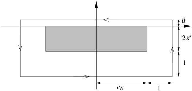
Figure 10: Integration path $\Gamma_{N}$. Here $c_{N}=2(N+1)\|\omega\|_{\infty}$, $\beta=\lambda^{2}$, and the shaded area contains all possible values of $\gamma(i;J)$ for momentum graphs with $N$ interaction vertices.

We then estimate $\Phi_{1}^{\lambda}(k_{0;\ell_{1}})\Phi_{1}^{\lambda}(-k^{\prime}_{0;\ell_{1}})\leq 1$ to remove the dependence on the two “amputated” interaction vertices at the bottom of the interaction trees. If there is any free momenta associated with these vertices, they will be integrated over next, resulting in an irrelevant factor of $1$.

Each of the resolvents in $\frac{1}{|z-\gamma_{i}|}$, $i\in A_{1}\cup A_{2}$, depends only on the free momenta associated with edges ending on a time slice $i^{\prime}\geq i$. Consider a degree one vertex in the plus-tree. By Proposition 5.2, there is a permutation $\pi$ of $\{0,1,2\}$ such that $\tilde{k}=k_{i-1,\ell_{i}+\pi(1)}$ is the free momentum, and neither $k_{i-1,\ell_{i}+\pi(3)}$ nor $k_{0}=k_{i-1,\ell_{i}+\pi(2)}+k_{i-1,\ell_{i}+\pi(1)}$ depend on $\tilde{k}$. We then estimate $\Phi_{1}^{\lambda}(k_{i-1;\ell_{i}})\leq F_{1}^{\lambda}(k_{0})$. Analogously, for every degree one vertex in the minus tree, we can estimate $\Phi_{1}^{\lambda}(-k^{\prime}_{i-1;\ell^{\prime}_{i}})\leq F_{1}^{\lambda}(-k^{\prime}_{0})$. We remove all remaining $\Phi_{1}^{\lambda}$, which are thus attached to a degree zero or two vertex, by the trivial estimate, $\Phi_{1}^{\lambda}\leq 1$.

After this we can use the estimates given in Lemmata 7.5 and 7.6 to iterate through the free momentum integrals in the direction of time, i.e., from bottom to top in the graph. At each iteration step, only one resolvent factor depends on the corresponding free momenta, and the remaining free momenta only affect the value of “$\alpha$” in the resolvent factor. The estimates can be used with $\beta=\lambda^{2}$ for those $z\in\Gamma_{N}$ in the top horizontal part of the path; we can ignore the imaginary part of $\gamma_{i}$, since this is always negative, and thus would only increase the “$\beta$” in the Lemmas and lower the value of the resolvent factor. For the remaining $z$ we have $|z-\gamma_{i}|\geq 1$, and the upper bounds remain valid also for these values of $z$, after we adjust the constant so that $C\geq 1$. After the last iteration step, there is one free momentum integral left, provided that there are any free momenta attached to the top fusion vertex. However, since the remaining integrand is momentum-independent, this integral yields a trivial factor $1$, and can thus be ignored. The only remaining integral is over $z$. This we estimate by

$$\oint_{\Gamma_{N}}\frac{|{\rm d}z|}{2\pi}\frac{{\rm e}^{s({\rm Im\,}z)_{+}}}{|z|}\leq C{\rm e}^{s\lambda^{2}}\langle\ln N\rangle\langle\ln\beta\rangle\,,$$ (8.5)

where $C$ is a constant which depends only on $\|\omega\|_{\infty}$. Collecting the estimates together yields the upper bound in (8.1); the power of $\lambda$ arising from the estimates is $2n-2(\tilde{n}_{0}-n^{\prime}_{0})-2n^{\prime}_{0}-b\tilde{n}_{1}$ which we have simplified to $2+\tilde{n}_{2}+(1-b)\tilde{n}_{1}-\tilde{n}_{0}$ using $2n-2=\tilde{n}_{0}+\tilde{n}_{1}+\tilde{n}_{2}$. ∎∎

For the following result, let us recall the definition of the time-dependent exponents in a main term, $\gamma(i)$ in equation (4.11). In the analysis of the partial integration error term, Section 8.3, we will need a generalization of this phase factor to a case with interactions also in the minus tree. To this end we define

$$\tilde{\gamma}({i;J})=\gamma^{+}_{j}+\gamma^{-}_{j^{\prime}},\quad\text{with}\quad j=J_{+}(i;J),\ j^{\prime}=J_{-}(i;J)\,,$$ (8.6)

where thus $j,j^{\prime}\in\{0,1,\ldots,n\}$. For the main term, with $n^{\prime}=0$, we have $J(i)=+1$, for all $i$, and $\gamma(i)=\tilde{\gamma}({i;1})$. Although the functional dependence on the mapping $J$ is different between $\tilde{\gamma}$ and the amputated $\gamma$, in both cases the correct exponential can be read off from our momentum graphs by summing over $\sigma_{e}\omega(k_{e})$, for all edges $e$ which intersect the corresponding time slice. Therefore, we will make no distinction between the amputated and non-amputated exponentials and denote both by $\gamma(i;J)$.

Lemma 8.2 (Basic $\mathcal{F}$-estimate)

There is a constant $C>0$ such that for any momentum graph $\mathcal{G}(S,J,n,\ell,n^{\prime},\ell^{\prime})$, $n,n^{\prime}\geq 0$, and $s>0$ we have

$$\lim_{\Lambda\to\infty}\lambda^{n+n^{\prime}}\sum_{\sigma\in\{\pm 1\}^{\mathcal{I}^{\prime}_{n}}}\sum_{\sigma^{\prime}\in\{\pm 1\}^{\mathcal{I}^{\prime}_{\smash[t]{n^{\prime}}}}}{\mathbbm{1}}(\sigma_{n,1}=1){\mathbbm{1}}(\sigma^{\prime}_{n^{\prime},1}=-1)$$

$$\quad\times\int_{(\Lambda^{*})^{\mathcal{I}^{\prime}_{n}}}\!{\rm d}k\,\int_{(\Lambda^{*})^{\mathcal{I}^{\prime}_{\smash[t]{n^{\prime}}}}}\!{\rm d}k^{\prime}\,\Delta_{n,\ell}(k,\sigma;\Lambda)\Delta_{n^{\prime},\ell^{\prime}}(k^{\prime},\sigma^{\prime};\Lambda)\prod_{A\in S}\delta_{\Lambda}\!\Bigl{(}\sum_{i\in A}K_{i}\Bigr{)}$$

$$\qquad\times\prod_{i=1}^{n}\Phi_{1}^{\lambda}(k_{i-1;\ell_{i}})\prod_{i=1}^{n^{\prime}}\Phi_{1}^{\lambda}(-k^{\prime}_{i-1;\ell^{\prime}_{i}})\left|\int_{({\mathbb{R}}_{+})^{I_{0,n+n^{\prime}}}}\!{\rm d}r\,\delta\Bigl{(}s-\sum_{i=0}^{n+n^{\prime}}r_{i}\Bigr{)}\prod_{i=0}^{n+n^{\prime}}{\rm e}^{-{\rm i}r_{i}\gamma({i;J})}\right|$$

$$\leq{\rm e}^{s\lambda^{2}}\frac{(s\lambda^{2})^{n_{0}}}{(n_{0})!}\lambda^{n_{2}+(1-b)n_{1}-n_{0}}C^{1+n_{1}+n_{2}}\langle\ln(n+n^{\prime}+1)\rangle\langle\ln\lambda\rangle^{1+n_{2}+2n_{1}}\,,$$ (8.7)

where $n_{i}$ denotes the number of interaction vertices of degree $i$.

Proof.

There are altogether $N=n+n^{\prime}$ interaction vertices, and for $j=0,1,2$ we set $A_{j}=\left\{0\leq i<N\left|\,\deg v_{i+1}=j\makebox[0.0pt]{$\displaystyle\phantom{0\leq i<N}$}\right.\!\right\}$ and $B=\emptyset$. With these adjustments, we can derive the bound as in the proof of Lemma 8.1. (Choosing $B=\emptyset$ implies $n^{\prime}_{0}=0$ and the estimate thus ignores any additional decay arising from factors with ${\rm Im\,}\gamma_{i}<0$.) The resulting power of $\lambda$ is $n+n^{\prime}-2n_{0}-bn_{1}$ which we have simplified using $n+n^{\prime}=n_{0}+n_{1}+n_{2}$. ∎∎

8.1 Amputated error term

Proposition 8.3

Suppose $t>0$ and $0<\lambda<\lambda^{\prime}_{0}$ are given, and define $N_{0}$ and $\kappa$, as in Definition 6.1. There is a constant $C>0$ depending only on $f$ and $g$, and $c>0$ depending only on $\omega$ such that

$$\limsup_{\Lambda\to\infty}|Q^{\rm err}_{\rm amp}[g,f](t)|^{2}\leq Ct^{2}{\rm e}^{t}\langle ct\rangle^{N_{0}}N_{0}^{2N_{0}+2}(4N_{0})!\langle\ln\lambda\rangle^{4N_{0}+2}\Bigl{(}\lambda+\lambda^{-2}N_{0}^{-b_{0}N_{0}/4}\Bigr{)}\,,$$ (8.8)

as soon as $N_{0}(\lambda)\geq 56$.

Since $\gamma^{\prime}\leq 1$, we can apply the limits (6.6) and (6.7) here and conclude from the above bound that $\limsup_{\Lambda\to\infty}|Q^{\rm err}_{\rm amp}[g,f](t)|\to 0$ as $\lambda\to 0$.

Proof.

By Proposition 3.3, and according to the discussion in Section 4.3, we have

$$\limsup_{\Lambda\to\infty}|Q^{\rm err}_{\rm amp}[g,f](t)|^{2}\leq C\|f\|_{2}^{2}t^{2}\lambda^{-4}$$

$$\times\sup_{0\leq s\leq t\lambda^{-2}}\limsup_{\Lambda\to\infty}\!\!\!\sum_{J\text{ interlaces }(n-1,n-1)}\sum_{\ell,\ell^{\prime}\in G_{n}}\sum_{S\in\pi(I_{4n+2})}|\mathcal{A}_{n}^{\rm ampl}(S,J,\ell,\ell^{\prime},s,\kappa)|\,,$$ (8.9)

where $n=N_{0}$. We have here first applied dominated convergence to move the limit $\limsup_{\Lambda\to\infty}$ inside the $s$-integral which was then estimated trivially. The bound for domination is contained in the following.

The $\limsup$ can be bounded by first employing (4.3) and then Lemma 8.1. This yields the bound

$$\|\hat{g}\|_{\infty}^{2}\sum_{J\text{ interlaces }(n-1,n-1)}\sum_{\ell,\ell^{\prime}\in G_{n}}\sum_{S\in\pi(I_{4n+2})}\prod_{A\in S}\sup_{\Lambda,k,\sigma}|C_{|A|}(\sigma,k;\lambda,\Lambda)|$$

$$\qquad\times{\rm e}^{s\lambda^{2}}\frac{(s\lambda^{2})^{\tilde{n}_{0}-n^{\prime}_{0}}}{(\tilde{n}_{0}-n^{\prime}_{0})!}\lambda^{2+\tilde{n}_{2}-\tilde{n}_{0}+(1-b)\tilde{n}_{1}}n^{-b_{0}n^{\prime}_{0}}C^{1+\tilde{n}_{1}+\tilde{n}_{2}}\langle\ln n\rangle\langle\ln\lambda\rangle^{1+\tilde{n}_{2}+2\tilde{n}_{1}}$$

$$\quad\leq\|\hat{g}\|_{\infty}^{2}\sum_{J\text{ interlaces }(n-1,n-1)}\sum_{\ell,\ell^{\prime}\in G_{n}}\sum_{S\in\pi(I_{4n+2})}\prod_{A\in S}\sup_{\Lambda,k,\sigma}|C_{|A|}(\sigma,k;\lambda,\Lambda)|$$

$$\qquad\times{\rm e}^{t}\langle ct\rangle^{n}\langle\ln\lambda\rangle^{2+4n}\lambda^{2+\tilde{n}_{2}-\tilde{n}_{0}+(1-b)\tilde{n}_{1}}n^{-b_{0}n^{\prime}_{0}}\,.$$ (8.10)

We have used here $\tilde{n}_{0}\leq n_{0}\leq n$ which is implied by Lemma 6.3. We set $r=2n+1-|S|$ as in Proposition 6.4, and note that here $\tilde{n}_{j}=n_{j}-n_{j}(2)\geq 0$ and $n^{\prime}_{0}=n_{0}(n{+}1)-n_{0}(2)$. By Lemma 6.3, $\tilde{n}_{2}-\tilde{n}_{0}=r+n_{0}(2)-n_{2}(2)\geq r-2$, and $\tilde{n}_{1}\geq n_{1}-2$. If $r+n_{1}\geq 24$, we thus have $\tilde{n}_{2}-\tilde{n}_{0}+(1-b)\tilde{n}_{1}\geq r+\frac{1}{4}n_{1}-3\geq 3$. In such cases we estimate $\lambda^{2+\tilde{n}_{2}-\tilde{n}_{0}+(1-b)\tilde{n}_{1}}n^{-b_{0}n^{\prime}_{0}}\leq\lambda^{5}$.

If $r+n_{1}<24$, we get from Proposition 6.4, the estimates $n^{\prime}_{0}\geq(n-n_{1}-r)/2-2$ and $\tilde{n}_{2}-\tilde{n}_{0}\geq 0$. Thus for any $n\geq 56$, we have $n^{\prime}_{0}\geq(n/2)-14\geq n/4$, and therefore also $\lambda^{2+\tilde{n}_{2}-\tilde{n}_{0}+(1-b)\tilde{n}_{1}}n^{-b_{0}n^{\prime}_{0}}\leq\lambda^{2}n^{-b_{0}n/4}$.

The number of terms in the sum over $J$ is less than $2^{2n-2}$ and the number of terms in the sum over $\ell$ is equal to $(2n{-}1)!!\leq(2n)^{n}$. For the sum over $S$ we can apply Lemma 7.3. Collecting all the estimates together proves that (8.8) holds, after readjustment of the constants $c$ and $C$. ∎∎

8.2 Constructive interference error terms

Proposition 8.4

Suppose $t>0$ and $0<\lambda<\lambda^{\prime}_{0}$ are given, and define $N_{0}$ and $\kappa$, as in Definition 6.1. There is a constant $C>0$ depending only on $f$ and $g$, and $c>0$ depending only on $\omega$ such that

$$\limsup_{\Lambda\to\infty}|Q^{\rm err}_{\rm cut}[g,f](t)|^{2}\leq Ct^{2}{\rm e}^{t}\langle ct\rangle^{N_{0}}N_{0}^{2N_{0}+4}(4N_{0})!\langle\ln\lambda\rangle^{4N_{0}+3}\lambda^{1/4}\,.$$ (8.11)

Since $\gamma^{\prime}\leq\frac{1}{4}$, this estimate proves that $\limsup_{\Lambda\to\infty}|Q^{\rm err}_{\rm amp}[g,f](t)|\to 0$ as $\lambda\to 0$.

Proof.

We again denote $\mathcal{I}^{\prime}_{n}=\mathcal{I}_{n}\cup\{(n,1)\}=\left\{(i,j)\left|\,0\leq i\leq n,1\leq j\leq m_{n-i}\makebox[0.0pt]{$\displaystyle\phantom{(i,j)}$}\right.\!\right\}$, and define $I=I_{2m_{n}}=I_{4n+2}$ to give labels to the final $\hat{a}$, as before. By expanding the pairing truncations in $\widehat{\mathcal{P}}$ to individual components, and then applying the cluster expansions in Lemma 4.2, we find that the effect of the extra terms in the truncations is the cancellation of all those terms from the main cumulant expansion which contain one of the corresponding pairings. None of the other clusterings is affected. The remainder of the analysis is completely analogous to that used for $\mathcal{A}_{n}$ in Section 4.3, and it shows that

$${\mathbb{E}}\Bigl{[}|\langle\hat{g},\mathcal{Z}_{n}(s,t/\varepsilon,\cdot,+1,\kappa)[\hat{a}_{s}]\rangle|^{2}\Bigr{]}$$

$$\quad=\sum_{J\text{ interlaces }(n-1,n-1)}\ \sum_{\ell,\ell^{\prime}\in G_{n}}\ \sum_{S\in\pi(I_{4n+2})}\mathcal{Z}_{n}^{\rm ampl}(S,J,\ell,\ell^{\prime},t/\varepsilon-s,\kappa)\,.$$ (8.12)

Here $\mathcal{Z}_{n}^{\rm ampl}(S,J,\ell,\ell^{\prime},s,\kappa)=0$ for any partition $S$ which contains a pairing of any two edges attached to one of the “truncated” vertices (i.e., if there are $A\in S$ and $i\in\{1,2\}$ such that $|A|=2$ and $\mathcal{E}_{+}(u)\subset\mathcal{E}_{-}(v_{i})$ for every $u\in A$). For all other $S$ we have

$$\mathcal{Z}_{n}^{\rm ampl}(S,J,\ell,\ell^{\prime},s,\kappa)=(-\lambda^{2})^{n}\sum_{\sigma,\sigma^{\prime}\in\{\pm 1\}^{\mathcal{I}^{\prime}_{n}}}\int_{(\Lambda^{*})^{\mathcal{I}^{\prime}_{n}}}\!{\rm d}k\,\int_{(\Lambda^{*})^{\mathcal{I}^{\prime}_{n}}}\!{\rm d}k^{\prime}\,$$

$$\quad\times\Delta_{n,\ell}(k,\sigma;\Lambda)\Delta_{n,\ell^{\prime}}(k^{\prime},\sigma^{\prime};\Lambda)\prod_{A\in S}\Bigl{[}\delta_{\Lambda}\!\Bigl{(}\sum_{i\in A}K_{i}\Bigr{)}C_{|A|}(o_{A},K_{A};\lambda,\Lambda)\Bigr{]}$$

$$\quad\times\sigma_{1,\ell_{1}}\Phi_{0}^{\lambda}(k_{0;\ell_{1}})\sigma^{\prime}_{1,\ell^{\prime}_{1}}\Phi_{0}^{\lambda}(-k^{\prime}_{0;\ell^{\prime}_{1}})\prod_{i=2}^{n}\Bigl{[}\sigma_{i,\ell_{i}}\Phi_{1}^{\lambda}(k_{i-1;\ell_{i}})\sigma^{\prime}_{i,\ell^{\prime}_{i}}\Phi_{1}^{\lambda}(-k^{\prime}_{i-1;\ell^{\prime}_{i}})\Bigr{]}$$

$$\quad\times{\mathbbm{1}}(\sigma_{n,1}=1){\mathbbm{1}}(\sigma^{\prime}_{n,1}=-1)|\hat{g}(k_{n,1})|^{2}\int_{({\mathbb{R}}_{+})^{I_{2,2n}}}\!{\rm d}r\,\delta\Bigl{(}s-\sum_{i=2}^{2n}r_{i}\Bigr{)}\prod_{i=2}^{2n}{\rm e}^{-{\rm i}r_{i}\gamma({i;J})}\,,$$ (8.13)

where $\gamma({i;J})$ is given by (4.3). We use the Schwarz inequality in the sum over $n$, and then proceed as in the proof of Proposition 8.3. Then using Proposition 3.3 yields the estimate

$$\limsup_{\Lambda\to\infty}|Q^{\rm err}_{\rm cut}[g,f](t)|^{2}\leq N_{0}C\|f\|_{2}^{2}t^{2}\lambda^{-4}\sup_{0\leq s\leq t\lambda^{-2}}\sum_{n=1}^{N_{0}}\sum_{J\text{ interlaces }(n-1,n-1)}$$

$$\qquad\times\sum_{\ell,\ell^{\prime}\in G_{n}}\sum_{S\in\pi(I_{4n+2})}\limsup_{\Lambda\to\infty}|\mathcal{Z}_{n}^{\rm ampl}(S,J,\ell,\ell^{\prime},s,\kappa)|\,.$$ (8.14)

Compared to the amputated error term, the terms in the sum have the following improved upper bounds whose proof will be given at the end of this section.

Lemma 8.5 (Basic $\mathcal{Z}$-estimate)

If we change the term $\Phi_{1}^{\lambda}(k_{0;\ell_{1}})\Phi_{1}^{\lambda}(-k^{\prime}_{0;\ell^{\prime}_{1}})$ on the left hand side of (8.1) to $\Phi_{0}^{\lambda}(k_{0;\ell_{1}})\Phi_{0}^{\lambda}(-k^{\prime}_{0;\ell^{\prime}_{1}})$, the estimate can either be improved by a factor of $C\langle\ln\lambda\rangle\lambda^{z_{0}}$, $z_{0}=bd-2$, or the corresponding $\mathcal{Z}_{n}^{\rm ampl}$ is zero. If $\tilde{n}_{1}=0$, then the estimate is valid also with $z_{0}=(d-2)b$. If any of the amputated vertices has degree two, the estimate is valid with $z_{0}=(d-1)b$.

The $\limsup$-factor can then be bounded by first employing (8.2) and then using Lemma 8.5. We neglect the extra decay provided by the partial time integration, and estimate $n^{-b_{0}n^{\prime}_{0}}\leq 1$. Simplifying the expression somewhat along the lines used in the proof of Proposition 8.3, we thus have the following bound for the $\limsup$-term:

$$\|\hat{g}\|_{\infty}^{2}\sum_{n=1}^{N_{0}}\sum_{J\text{ interlaces }(n-1,n-1)}\sum_{\ell,\ell^{\prime}\in G_{n}}\sum_{S\in\pi(I_{4n+2})}\prod_{A\in S}\sup_{\Lambda,k,\sigma}|C_{|A|}(\sigma,k;\lambda,\Lambda)|$$

$$\qquad\times{\rm e}^{t}\langle ct\rangle^{n}\langle\ln\lambda\rangle^{3+4n}\lambda^{2+\tilde{n}_{2}-\tilde{n}_{0}+(1-b)\tilde{n}_{1}+db}$$

$$\qquad\times{\mathbbm{1}}(\mathcal{Z}_{n}^{\rm ampl}\neq 0)\times\begin{cases}\lambda^{-b},&\text{if }n_{2}(2)>0;\\ \lambda^{-2b},&\text{if }n_{2}(2)=0,\tilde{n}_{1}=0;\\ \lambda^{-2},&\text{otherwise.}\\ \end{cases}$$ (8.15)

By Proposition 6.4, here always $\tilde{n}_{2}-\tilde{n}_{0}\geq 0$ and $\tilde{n}_{1}\geq 0$. Thus if $n_{2}(2)>0$, the power of $\lambda$ can be bounded from above by $\lambda^{2+b(d-1)}\leq\lambda^{4+\frac{1}{4}}$.

We can thus assume that $n_{2}(2)=0$. Then $\tilde{n}_{2}-\tilde{n}_{0}=n_{2}-n_{0}-n_{2}(2)+n_{0}(2)=r+n_{0}(2)$. If also $n_{0}(2)=0$, then necessarily $n_{1}(2)=2$, i.e., that both amputated interaction vertices have exactly one free momentum attached to them. By the iterative cluster scheme, this implies that there is a cluster $A_{0}\in S$ such that exactly two of the edges in the first interaction vertex, the amputated minus vertex, connect to it. If $A_{0}$ is a pairing, then $\mathcal{Z}_{n}^{\rm ampl}=0$ by definition. Otherwise, $|A_{0}|\geq 4$, and thus then $r\geq 1$. Therefore, in all cases we can conclude that now either $\mathcal{Z}_{n}^{\rm ampl}=0$ or $\tilde{n}_{2}-\tilde{n}_{0}\geq 1$.

Therefore, if $n_{2}(2)=0$ and $\tilde{n}_{1}=0$, the power of $\lambda$ is bounded by $\lambda^{2+1+b(d-2)}\leq\lambda^{4+\frac{1}{2}}\leq\lambda^{4+\frac{1}{4}}$. If $n_{2}(2)=0$ and $\tilde{n}_{1}>0$, then the bound $\lambda^{2+1+1-b+db-2}=\lambda^{2+b(d-1)}\leq\lambda^{4+\frac{1}{4}}$ can be used. Therefore, whatever the clustering, a bound $\lambda^{4+\frac{1}{4}}$ is always available. The rest of the sums can be bounded exactly as in the proof of Proposition 8.3, apart from the first sum over $n$ which yields an additional factor $N_{0}$. Collecting all the estimates together proves that (8.11) holds. ∎∎

• Proof of Lemma 8.5  The statement with $z_{0}=0$ is a corollary of the proof of Lemma 8.1, since the estimate $\Phi_{0}^{\lambda}(k_{0;\ell_{1}})\Phi_{0}^{\lambda}(-k^{\prime}_{0;\ell^{\prime}_{1}})\leq 1$ allows to remove these terms at the right place in the proof. However, we can improve on the estimate by using the fact that $\Phi_{0}^{\lambda}(k_{0;\ell_{1}})$ enforces particular sums of momenta to lie very close to the singular manifold.

  Let us first consider the case were one of the amputated vertices has degree two. If this is the amputated minus vertex, we find from Proposition 3.1 that

  $$\Phi_{0}^{\lambda}(-k^{\prime}_{0;\ell^{\prime}_{1}})\leq\sum_{e_{1},e_{2}\in\mathcal{E}_{-}(v_{1});\ e_{1}<e_{2}}{\mathbbm{1}}\!\left(d(-(k_{e_{1}}+k_{e_{2}}),M^{\rm sing})<\lambda^{b}\right)\,.$$ (8.16)

  By Lemma 5.6, for any choice of $e_{1}$, $e_{2}$ here $-(k_{e_{1}}+k_{e_{2}})$ depends on the free momenta $k,k^{\prime}$ of $v_{1}$ either as $k$, $k^{\prime}$, or $-(k+k^{\prime})$. Thus when we first integrate over $k$ and then over $k^{\prime}$, in one of the integrals we can apply Lemma 7.1, according to which

  $$\sup_{k_{0}\in{\mathbb{T}}^{d}}\int_{{\mathbb{T}}^{d}}{\rm d}k\,{\mathbbm{1}}\!\left(d(\pm k+k_{0},M^{\rm sing})<\lambda^{b}\right)\leq C\lambda^{b(d-1)}\,.$$ (8.17)

  After this we can estimate $\Phi_{0}^{\lambda}(k_{0;\ell_{1}})\leq 1$, and then continue as in the proof of Lemma 8.1.

  If the amputated minus vertex does not have degree two, we estimate trivially $\Phi_{0}^{\lambda}(-k^{\prime}_{0;\ell^{\prime}_{1}})\leq 1$ and integrate over any free momenta attached to it, which yields an irrelevant factor of one for the iterative bound. We then estimate the extra factor in the amputated plus vertex by

  $$\Phi_{0}^{\lambda}(k_{0;\ell_{1}})\leq\sum_{e_{1},e_{2}\in\mathcal{E}_{-}(v_{2});\ e_{1}<e_{2}}{\mathbbm{1}}\!\left(d(k_{e_{1}}+k_{e_{2}},M^{\rm sing})<\lambda^{b}\right)\,.$$ (8.18)

  If the amputated plus vertex, $v_{2}$, has degree two, we again gain a factor $C\lambda^{b(d-1)}$ from performing the two free integrations attached to it. After this the proof can proceed as in Lemma 8.1. Thus if either of the amputated vertices has degree two, we have proven a gain by the stated factor with $z_{0}=b(d-1)$. This proves the last statement made in the Lemma.

  To prove the other two statements, it is sufficient to consider the term corresponding to some fixed pair $e_{1}<e_{2}$, $e_{1},e_{2}\in\mathcal{E}_{-}(v_{2})$ in the bound (8.18). If $k_{e_{1}}+k_{e_{2}}$ is independent of all free momenta, then by Proposition 5.10, the two initial time vertices belonging to $e_{1}\cup e_{2}$ must be isolated from the rest of the initial time vertices. This is possible only if they are paired, but then $\mathcal{Z}_{n}^{\rm ampl}=0$ by definition. Thus we can assume that there is some free momenta on which $k_{e_{1}}+k_{e_{2}}$ depends. Of the corresponding free edges, let $f_{0}$ denote the one added first (i.e., it is the maximum in the ordering of edges).

  We next estimate all $\Phi_{1}^{\lambda}$-factors as in the proof of Lemma 8.1, with one exception: if the fusion vertex at which $f_{0}$ ends is a degree two interaction vertex, we will need the corresponding $\Phi_{1}^{\lambda}$-factor, and this is kept unchanged. Then we use the estimates in the proof of Lemma 8.1, and iterate through the interaction vertices until the vertex at which $f_{0}$ ends is reached. If $f_{0}$ is attached to either an amputated interaction vertex or the top fusion vertex, then using (8.17) we gain an improvement with $z_{0}=b(d-1)$, which is the best bound of all the three possibilities.

  If $f_{0}$ is attached to a degree one non-amputated interaction vertex, we first remove the corresponding “resolvent” factor using the trivial $L^{\infty}$ estimate and then apply (8.17). Since in the proof of Lemma 8.1 this term would be estimated by $C\langle\ln\lambda\rangle^{2}\lambda^{-b}$, we gain an improvement by a factor of $C\lambda^{b-2+b(d-1)}$, as compared to Lemma 8.1. This yields the worst bound with $z_{0}=bd-2$.

  Otherwise, $f_{0}$ is attached to a non-amputated interaction vertex of degree two. Let the two free momenta be denoted by $k_{1}$ and $k_{2}$, and the third integrated momenta by $k_{3}$. In addition, denote $k_{0}=k_{1}+k_{2}+k_{3}$ which is independent of $k_{1}$ and $k_{2}$. By Lemma 5.6, $k_{e_{1}}+k_{e_{2}}=\pm k_{i}+k_{0}^{\prime}$, for some choice of sign and $i\in\{1,2,3\}$, where $k_{0}^{\prime}$ is independent of $k_{1}$, $k_{2}$. Thus we need to consider

  $$\int_{({\mathbb{T}}^{d})^{2}}\!{\rm d}k_{1}{\rm d}k_{2}\,{\mathbbm{1}}\!\left(d(\pm k_{i}+k_{0}^{\prime},M^{\rm sing})<\lambda^{b}\right)$$

  $$\quad\times\frac{\Phi_{1}^{\lambda}(\pm(k_{1},k_{2},k_{0}-k_{1}-k_{2}))}{|\omega(k_{1})+\sigma^{\prime}\omega(k_{2})+\sigma\omega(k_{0}-k_{1}-k_{2})-\alpha+{\rm i}\beta|}\,.$$ (8.19)

  (The $\Phi_{1}^{\lambda}$-factor is present here, as the only one which was not estimated trivially. $\Phi_{1}^{\lambda}$ is also clearly invariant under permutation of its arguments.) If $i=1$, we estimate $\Phi_{1}^{\lambda}\leq F_{1}^{\lambda}(\pm(k_{0}-k_{1}))$, and change the integration variable $k_{1}$ to $k=\pm k_{1}+k_{0}^{\prime}$. Then first applying Lemma 7.5 to the $k_{2}$ integral and then (8.17) to the $k$ integral, we find that the integral is bounded by $C\langle\ln\beta\rangle^{2}\lambda^{-b+b(d-1)}$. Analogous chance of variables can be done to show that the bound is valid also if $i=2$ or $i=3$. Thus we get an improvement by a factor of $C\langle\ln\beta\rangle\lambda^{b(d-2)}$ compared to the estimate used in the proof of Lemma 8.1.

  After one of the above estimates, we can finish the iteration of the interaction vertices, and complete the rest of the proof as in Lemma 8.1. If $\tilde{n}_{1}=0$, then there are no non-amputated degree one vertices. Thus either of the two better estimates apply, and $z_{0}=b(d-2)>bd-2$ can be used. Otherwise, we need to resort to the worst estimate with $z_{0}=bd-2$. This completes the proof of the Lemma.∎

8.3 Partial time-integration error terms

Proposition 8.6

Suppose $t>0$ and $0<\lambda<\lambda^{\prime}_{0}$ are given, and define $N_{0}$ and $\kappa$, as in Definition 6.1. There is a constant $C>0$ depending only on $f$ and $g$, and $c>0$ depending only on $\omega$ and $\lambda^{\prime}_{0}$ such that

$$\limsup_{\Lambda\to\infty}|Q^{\rm err}_{\rm pti}[g,f](t)|^{2}\leq Ct^{2}{\rm e}^{t}\langle ct\rangle^{N_{0}}N_{0}^{2N_{0}+5+2b_{0}}(4N_{0})!\langle\ln\lambda\rangle^{4N_{0}+2}\lambda^{1/4}$$

$$\quad+Ct^{2}N_{0}^{2+2b_{0}}\sup_{\begin{subarray}{c}0\leq s\leq t\lambda^{-2},\\ N_{0}/2\leq n<N_{0}\end{subarray}}\ \sum_{J\text{ interlaces }(n,n)}\ \sum_{\ell,\ell^{\prime}\in G_{n}}\ \sum_{S\in\pi(I_{4n+2})}|\mathcal{G}_{n}^{\rm pairs}(S,J,\ell,\ell^{\prime},s,\kappa)|\,,$$ (8.20)

where $\mathcal{G}_{n}^{\rm pairs}(S,J,\ell,\ell^{\prime},s,\kappa)=0$, if the graph defined by $J,S,\ell,\ell^{\prime}$ is not fully paired, and otherwise it is equal to

$$\mathcal{G}_{n}^{\rm pairs}(S,J,\ell,\ell^{\prime},s,\kappa)=(-\lambda^{2})^{n}\sum_{\sigma,\sigma^{\prime}\in\{\pm 1\}^{\mathcal{I}^{\prime}_{n}}}\int_{({\mathbb{T}}^{d})^{\mathcal{I}^{\prime}_{n}}}\!{\rm d}k\,\int_{({\mathbb{T}}^{d})^{\mathcal{I}^{\prime}_{n}}}\!{\rm d}k^{\prime}\,\Delta_{n,\ell}(k,\sigma)\Delta_{n,\ell^{\prime}}(k^{\prime},\sigma^{\prime})$$

$$\quad\times\prod_{A=\{i,j\}\in S}\Bigl{[}\delta(K_{i}+K_{j}){\mathbbm{1}}(o_{i}=-o_{j})W(K_{i})\Bigr{]}\prod_{i=1}^{n}\Bigl{[}\sigma_{i,\ell_{i}}\Phi_{1}^{\lambda}(k_{i-1;\ell_{i}})\sigma^{\prime}_{i,\ell^{\prime}_{i}}\Phi_{1}^{\lambda}(-k^{\prime}_{i-1;\ell^{\prime}_{i}})\Bigr{]}$$

$$\quad\times{\mathbbm{1}}(\sigma_{n,1}=1){\mathbbm{1}}(\sigma^{\prime}_{n,1}=-1)|\hat{g}(k_{n,1})|^{2}\int_{({\mathbb{R}}_{+})^{I_{0,2n}}}\!{\rm d}r\,\delta\Bigl{(}s-\sum_{i=0}^{2n}r_{i}\Bigr{)}\prod_{i=0}^{2n}{\rm e}^{-{\rm i}r_{i}\gamma({i;J})}\,.$$ (8.21)

Proof.

The error term $\mathcal{G}_{n}$ was defined in (3.25), where we can directly apply (4.3). Comparing the result to the definition of $\mathcal{F}_{n}$ in (3) shows that

$$\langle\hat{g},\mathcal{G}_{n}(s,t,\cdot,1,\kappa)[\hat{a}_{s}]\rangle=\langle\hat{g},{\rm e}^{{\rm i}s\omega^{\lambda}}\mathcal{F}_{n}(t-s,\cdot,1,\kappa)[\hat{\psi}_{s}]\rangle\,.$$ (8.22)

Thus in this case

$${\mathbb{E}}\Bigl{[}|\langle\hat{g},\mathcal{G}_{n}(s,t/\varepsilon,\cdot,1,\kappa)[\hat{a}_{s}]\rangle|^{2}\Bigr{]}={\mathbb{E}}\Bigl{[}|\langle{\rm e}^{-{\rm i}s\omega^{\lambda}}\hat{g},\mathcal{F}_{n}(t/\varepsilon-s,\cdot,1,\kappa)[\hat{\psi}_{0}]\rangle|^{2}\Bigr{]}$$

$$\quad=\sum_{J\text{ interlaces }(n,n)}\ \sum_{\ell,\ell^{\prime}\in G_{n}}\ \sum_{S\in\pi(I_{4n+2})}\mathcal{G}_{n}^{\rm ampl}(S,J,\ell,\ell^{\prime},t/\varepsilon-s,\kappa)\,,$$ (8.23)

where

$$\mathcal{G}_{n}^{\rm ampl}(S,J,\ell,\ell^{\prime},s,\kappa)=(-\lambda^{2})^{n}\sum_{\sigma,\sigma^{\prime}\in\{\pm 1\}^{\mathcal{I}^{\prime}_{n}}}\int_{(\Lambda^{*})^{\mathcal{I}^{\prime}_{n}}}\!{\rm d}k\,\int_{(\Lambda^{*})^{\mathcal{I}^{\prime}_{n}}}\!{\rm d}k^{\prime}\,$$

$$\quad\times\Delta_{n,\ell}(k,\sigma;\Lambda)\Delta_{n,\ell^{\prime}}(k^{\prime},\sigma^{\prime};\Lambda)\prod_{A\in S}\Bigl{[}\delta_{\Lambda}\!\Bigl{(}\sum_{i\in A}K_{i}\Bigr{)}C_{|A|}(o_{A},K_{A};\lambda,\Lambda)\Bigr{]}$$

$$\quad\times\prod_{i=1}^{n}\Bigl{[}\sigma_{i,\ell_{i}}\Phi_{1}^{\lambda}(k_{i-1;\ell_{i}})\sigma^{\prime}_{i,\ell^{\prime}_{i}}\Phi_{1}^{\lambda}(-k^{\prime}_{i-1;\ell^{\prime}_{i}})\Bigr{]}{\mathbbm{1}}(\sigma_{n,1}=1){\mathbbm{1}}(\sigma^{\prime}_{n,1}=-1)|\hat{g}(k_{n,1})|^{2}$$

$$\quad\times\int_{({\mathbb{R}}_{+})^{I_{0,2n}}}\!{\rm d}r\,\delta\Bigl{(}s-\sum_{i=0}^{2n}r_{i}\Bigr{)}\prod_{i=0}^{2n}{\rm e}^{-{\rm i}r_{i}\gamma({i;J})}\,.$$ (8.24)

Thus the amplitude differs from the “amputated” amplitudes $\mathcal{A}_{n}$ and $\mathcal{Z}_{n}$ by containing also the propagators associated with the first two interactions. We recall the discussion about the definition of the non-amputated exponentials $\gamma(i;J)$ in (8.6).

As in the proof of Proposition 8.4, we then find

$$\limsup_{\Lambda\to\infty}|Q^{\rm err}_{\rm pti}[g,f](t)|^{2}\leq N_{0}^{2}(\kappa^{\prime})^{2}C\|f\|_{2}^{2}t^{2}\lambda^{-4}\sup_{0\leq s\leq t\lambda^{-2},N_{0}/2\leq n\leq N_{0}}$$

$$\quad\times\sum_{J\text{ interlaces }(n,n)}\ \sum_{\ell,\ell^{\prime}\in G_{n}}\sum_{S\in\pi(I_{4n+2})}\limsup_{\Lambda\to\infty}|\mathcal{G}_{n}^{\rm ampl}(S,J,\ell,\ell^{\prime},s,\kappa)|\,.$$ (8.25)

For any graph which is not fully paired, we take absolute values up to the time-integrations and apply Lemma 8.2. Using the notations of Lemma 6.3, then

$$|\mathcal{G}_{n}^{\rm ampl}(S,J,\ell,\ell^{\prime},s,\kappa)|$$

$$\quad\leq\|\hat{g}\|_{\infty}^{2}{\rm e}^{t}\frac{t^{n_{0}}}{(n_{0})!}\lambda^{r+(1-b)n_{1}}C^{2n+1}\langle\ln\lambda\rangle^{2+4n}\prod_{A\in S}\sup_{\Lambda,k,\sigma}|C_{|A|}(\sigma,k;\lambda,\Lambda)|\,.$$ (8.26)

If the graph is higher order, $r\geq 1$, and if the graph is not fully paired, $n_{1}\geq 1$. Thus for both types of graphs, and trivially for irrelevant graphs, we can use a bound

$$\lambda^{1/4}\|\hat{g}\|_{\infty}^{2}{\rm e}^{t}\langle ct\rangle^{n}\langle\ln\lambda\rangle^{2+4n}\prod_{A\in S}\sup_{\Lambda,k,\sigma}|C_{|A|}(\sigma,k;\lambda,\Lambda)|\,.$$ (8.27)

Consider then a fully paired graph. In this case, all clusters are pairings with $C_{2}((\sigma^{\prime},\sigma),(k^{\prime},k))={\mathbbm{1}}(\sigma^{\prime}+\sigma=0)W^{\lambda}_{\Lambda}(\sigma k)$. By Lemma 2.6, $W^{\lambda}_{\Lambda}(k)=W(k)+\Delta$, where $\limsup_{\Lambda\to\infty}\sup_{k\in{\mathbb{T}}^{d}}|\Delta|\leq 2c_{0}^{2}\lambda$. Since $W(-k)=W(k)$, we have for any finite index set $I$

$$\limsup_{\Lambda\to\infty}\Bigl{|}\prod_{i\in I}W^{\lambda}_{\Lambda}(\pm k_{i})-\prod_{i\in I}W(k_{i})\Bigr{|}\leq|I|C^{|I|-1}2c_{0}^{2}\lambda\,,$$ (8.28)

where $C=2c_{0}^{2}\lambda^{\prime}_{0}+\|W\|_{\infty}<\infty$. (The statement can be proven by induction in $|I|$.)

If $S$ is a pairing, we have $|S|=2n+1$, and applying Lemma 8.2, we can thus exchange in the definition of $\mathcal{G}_{n}^{\rm ampl}$ all $C_{2}$ terms by $W(K_{i}){\mathbbm{1}}(o_{i}=-o_{j})$ with an error whose $\limsup$ is bounded by

$$Cn\|\hat{g}\|_{\infty}^{2}{\rm e}^{t}\langle ct\rangle^{n}\langle\ln\lambda\rangle^{2+4n}\lambda\,.$$ (8.29)

In the resulting formula, we first resolve all $\delta_{\Lambda}$-functions as explained before. The summations over the free momenta are then turned into Lebesgue integrals as explained in Section 2.4, with an integrand which is uniformly bounded and has a pointwise limit when $\Lambda\to\infty$. By dominated convergence we can thus take the limit $\Lambda\to\infty$ inside the integrals which shows that the limit is given by $\mathcal{G}_{n}^{\rm pairs}$ defined in (8.6).

Now collecting all the above bounds together, estimating the number of terms in the $J,\ell,\ell^{\prime},S$ sums as before, readjusting $c$ and $C$ whenever necessary, and using $N_{0}^{2}(\kappa^{\prime})^{2}\lambda^{-4}=N_{0}^{2+2b_{0}}$, proves that (8.6) holds. ∎∎

8.4 Main term

We recall the graphical representation of the main term, and the related notations, in particular, Proposition 4.3 and the definition of $\gamma(m)$ in (4.11).

Proposition 8.7

Suppose $t>0$ and $0<\lambda<\lambda^{\prime}_{0}$ are given, and define $N_{0}$ and $\kappa$, as in Definition 6.1. There is a constant $C>0$ depending only on $f$ and $g$, and $c>0$ depending only on $\omega$ and $\lambda^{\prime}_{0}$ such that

$$\limsup_{\Lambda\to\infty}|Q^{\rm main}[g,f](t)-Q^{\rm pairs}[g,f](t)|\leq C{\rm e}^{t}\langle ct\rangle^{N_{0}}N_{0}^{N_{0}+4}(2N_{0})!\langle\ln\lambda\rangle^{2N_{0}+2}\lambda^{1/4}\,,$$ (8.30)

where $Q^{\rm pairs}$ is defined by

$$Q^{\rm pairs}[g,f](t)=\sum_{n=0}^{N_{0}-1}\sum_{\ell\in G_{n}}\sum_{S\in\pi(I_{0,2n+1})}\mathcal{F}_{n}^{\rm pairs}(S,\ell,t/\varepsilon,\kappa)$$ (8.31)

with $\mathcal{F}_{n}^{\rm pairs}(S,\ell,t/\varepsilon,\kappa)=0$, if the graph defined by $S,\ell$ is not fully paired, and otherwise it is equal to

$$\mathcal{F}_{n}^{\rm pairs}(S,\ell,t/\varepsilon,\kappa)=(-{\rm i}\lambda)^{n}\sum_{\sigma\in\{\pm 1\}^{\mathcal{I}^{\prime\prime}_{n}}}\int_{({\mathbb{T}}^{d})^{\mathcal{I}^{\prime\prime}_{n}}}\!{\rm d}k\,\Delta_{n,\ell}(k,\sigma)\hat{g}(k_{n,1})^{*}\hat{f}(k_{n,1})$$

$$\quad\times{\mathbbm{1}}(\sigma_{n,1}=1){\mathbbm{1}}(\sigma_{0,0}=-1)\prod_{A=\{i,j\}\in S}\!\Bigl{[}\delta(k_{0,i}+k_{0,j}){\mathbbm{1}}(\sigma_{0,i}=-\sigma_{0,j})W(k_{0,i})\Bigr{]}$$

$$\quad\times\prod_{i=1}^{n}\Bigl{[}\sigma_{i,\ell_{i}}\Phi_{1}^{\lambda}(k_{i-1;\ell_{i}})\Bigr{]}\int_{({\mathbb{R}}_{+})^{I_{0,n}}}\!{\rm d}r\,\delta\Bigl{(}t\lambda^{-2}-\sum_{i=0}^{n}r_{i}\Bigr{)}\prod_{m=0}^{n}{\rm e}^{-{\rm i}r_{m}\gamma(m)}\,.$$ (8.32)

Proof.

We can apply Lemma 8.2 with $n^{\prime}=0$ to estimate $|\mathcal{F}_{n}^{\rm ampl}(S,\ell,t/\varepsilon,\kappa)|$. The steps of the proof are otherwise identical to those used in the proof of Proposition 8.6. To avoid repetition, we skip the rest of the details here. ∎∎

9 Fully paired graphs

By the results proven in the previous section, only fully paired graphs remain to be estimated, with the corresponding amplitudes given by $\mathcal{G}_{n}^{\rm pairs}$ and $\mathcal{F}_{n}^{\rm pairs}$. In these terms, all sums over $\Lambda^{*}$ have already been replaced by integrals over ${\mathbb{T}}^{d}$, and we have changed the covariance function to its $\lambda\to 0$ limiting value. The related momentum graphs differ by the number of interactions in the minus tree: for $\mathcal{F}_{n}^{\rm pairs}$, we have $n^{\prime}=0$, and for $\mathcal{G}_{n}^{\rm pairs}$, $n^{\prime}=n$. For such relevant graphs, we have $r=0$ and $n_{1}=0$, and thus by Proposition 6.4 for any $1\leq i\leq n+n^{\prime}$,

$$n_{2}(i)\leq n_{0}(i)\quad\text{and}\quad n_{0}(i)\geq\frac{i}{2}\,.$$ (9.1)

In addition, by Lemma 6.3 also $n_{2}=n_{0}=\frac{n+n^{\prime}}{2}$. Since $n+n^{\prime}$ must then be even this implies that any $\mathcal{F}_{n}^{\rm pairs}$ with odd $n$ is zero. Also necessarily $\deg v_{1}=0$ and $\deg v_{n+n^{\prime}}=2$. Therefore, we can conclude that either the degrees of the interaction vertices form an alternating sequence $(0,2,0,2,\ldots,0,2)$, or this alternating behavior ends in two or more consecutive zeroes somewhere in the middle of the whole sequence.

Moreover, the first phase is always zero, since by Lemma 4.4 for any relevant graph

$${\rm Re\,}\gamma(0;J)=\sum_{i=1}^{2n+1}\!\!\sigma_{0,i}\omega(k_{0,i})+\sum_{i=1}^{2n^{\prime}+1}\!\!\sigma^{\prime}_{0,i}\omega(k^{\prime}_{0,i})$$ (9.2)

and the pairing of momenta and parities on the initial time slice implies that the terms cancel each other pairwise. For simplicity, let us now drop the dependence on $J$ from the notation, i.e., we denote $\gamma(m)$ instead of $\gamma(m;J)$ also for $\mathcal{G}_{n}^{\rm pairs}$. We recall that the time slice $m<N$ is called long, if $\deg v_{m+1}=0$. We now say that a long time slice $m$ is trivial, if additionally ${\rm Re\,}\gamma(m)=0$. Thus, for instance, the time slice $m=0$ is long and trivial in every relevant pairing graph. We also need to consider the index of the last trivial long time slice, by which we mean the last trivial long time slice in the initial sequence of trivial long slices: the index is defined as

$$m^{\prime}_{0}=\max\left\{0\leq m\leq N\left|\,{\rm Re\,}\gamma(j)=0\text{ if }0\leq j\leq m\text{ and the slice }j\text{ is long}\makebox[0.0pt]{$\displaystyle\phantom{0\leq m\leq N}$}\right.\!\right\},$$ (9.3)

where we have again set $N=n+n^{\prime}$. For relevant fully paired graphs, $0\leq m^{\prime}_{0}\leq N$, and we will soon show that $m^{\prime}_{0}=N$ if and only if the graph is leading.

Every degree two interaction vertex $v$ is at the top of the domain of influence of its two free momenta. We denote these by $f_{1},f_{2}$, with $f_{1}<f_{2}$, and let $e_{3}$ denote the third (integrated) edge in $\mathcal{E}_{-}(v)$, and $e_{0}$ the unique edge in $\mathcal{E}_{+}(v)$. We typically also denote $k_{1}=k_{f_{1}}$, $k_{2}=k_{f_{2}}$, $k_{3}=k_{e_{3}}$, and $k_{0}=k_{e_{0}}$. In particular, then $k_{3}=k_{0}-k_{1}-k_{2}$ uniformly in the free momenta.

Consider the two loops associated with $f_{1}$ and $f_{2}$ which would be created in the spanning tree by the addition of the edge. We travel the loops starting from the edge $f_{i}$ and finishing with the edge $e_{3}$. There is a unique vertex $v^{\prime}$ where the two loops meet (this is the first vertex in common between the two paths). The vertex $v^{\prime}$ is called the X-vertex, or crossing-vertex, associated with the double-loop of $v$. Clearly, $v^{\prime}$ must belong to at least three distinct integrated edges, and thus it has to be a degree zero interaction vertex. The remaining vertices (if there are any) along the two loops are called $T$-vertices, or through-vertices, of the double-loop of $v$. These are classified according to which of the three possible combinations of the free momenta appear in that vertex: if the vertex belongs to the path from $v\to v^{\prime}$ containing $f_{1}$, it is called a $T_{1}$-vertex; if to the path from $v\to v^{\prime}$ containing $f_{2}$, $T_{2}$-vertex; if to the path from $v^{\prime}\to v$, $T_{3}$-vertex. The names are explained by the following observation: if $w$ is a $T_{n}$-vertex, $n=1,2,3$, then exactly two of the momenta $k_{e}$, $e\in\mathcal{E}(w)$, depend on $k_{f_{1}}$ or $k_{f_{2}}$, and the dependence occurs via $\pm k_{n}$. The graph in Fig. 11 illustrates these definitions.

Figure 11: Example of a crossing graph. (Although this graph does not directly appear in our expansions, it could be completed to such a graph by adding a loss motive to the top of the graph.) The graph has two double-loops: the double-loop of $v_{3}$, for which $v_{1}$ is an $X$-vertex and $v_{2}$ is a $T_{3}$-vertex, and the double-loop of $v_{4}$, for which $v_{2}$ is an $X$-vertex and $v_{3}$ is a $T_{3}$-vertex. By inserting the appropriate parities for each edge, one can check the pairwise cancellation of phase factors on the time slice $0$, i.e., that ${\rm Re\,}\gamma(0)=0$. Under the graph, we have denoted explicitly the parities and momenta of each of the edges intersecting the time slice $1$. This shows that ${\rm Re\,}\gamma(1)=-\omega(k^{\prime})-\omega(k_{1})+\omega(k_{2})+\omega(-k^{\prime}-k_{1}-k_{2})\neq\Omega_{3}=-\omega(k_{0})-\omega(k_{1})+\omega(k_{2})+\omega(k_{0}-k_{1}-k_{2})$, with $k_{0}=-k^{\prime}-k_{1}^{\prime}-k_{2}^{\prime}$. Thus the time slice $1$ is long and independent of the double-loop of $v_{4}$ but it propagates a crossing with the double-loop of $v_{3}$.

Consider the interaction phase at an interaction vertex $v_{i}$, $1\leq i\leq N$,

$$\Omega_{i}:=\Omega(k_{\mathcal{E}_{-}(v_{i})},\sigma_{\mathcal{E}_{+}(v_{i})}).$$ (9.4)

Since now ${\rm Re\,}\gamma(0)=0$, for every time slice $m$ of a fully paired graph, $0\leq m\leq N$, we have

$${\rm Re\,}\gamma(m)=\sum_{i=m+1}^{N}\Omega_{i}=-\sum_{i=1}^{m}\Omega_{i}\,.$$ (9.5)

Consider an arbitrary long time slice $m$, $0\leq m\leq N-1$, which thus ends in a degree zero interaction vertex $v_{m+1}$, and an arbitrary degree two vertex $v_{i_{2}}$, with the corresponding free momenta $k_{1},k_{2}$. If ${\rm Re\,}\gamma(m)$ does not depend on $k_{1}$ or $k_{2}$, the time slice $m$ is said to be independent of the double-loop of $v_{i_{2}}$. If ${\rm Re\,}\gamma(m)$ depends on $k_{1}$ or $k_{2}$, but ${\rm Re\,}\gamma(m)-\Omega_{i_{2}}$ does not, the time slice is said to be nested inside the double-loop of $v_{i_{2}}$. If both ${\rm Re\,}\gamma(m)$ and ${\rm Re\,}\gamma(m)-\Omega_{i_{2}}$ depend on $k_{1}$ or $k_{2}$, the time slice $m$ is said to propagate a crossing with the double-loop of $v_{i_{2}}$.

We are now ready to give the precise definition of how the subleading relevant fully paired graphs are divided into nested and crossing graphs. We iterate trough degree two vertices, starting from the bottom of the graph, and consider the double-loop associated with the vertex. If every long time slice is independent of the double-loop, we move on to the next vertex in the list (we will soon prove that the double-loop is then formed by iteration of leading motives). Otherwise, there is a long time slice which depends on the double-loop. If all such time slices are nested inside the double-loop, the double-loop is called a nest and the graph is called nested. We have given an example of a nested graph in Fig. 12. Otherwise, there is a long time slice which depends on the double-loop but is not nested inside it. We call the topmost of these time slices the last propagated crossing slice, and the graph itself is then called a crossing graph. An example is given in Fig. 11.

Figure 12: Example of a nested graph. The graph has two double-loops: the double-loop of $v_{3}$, for which $v_{1}$ is an $X$-vertex, and the double-loop of $v_{4}$, for which $v_{2}$ is an $X$-vertex. Reading the appropriate parities and momenta from the graph shows that ${\rm Re\,}\gamma(1)=-\omega(k^{\prime})-\omega(k_{1})+\omega(k_{2})+\omega(k_{3})=\Omega_{3}$. Thus the time slice $1$ is long and independent of the double-loop of $v_{4}$ but it is nested inside the double-loop of $v_{3}$.

The following Proposition shows that these definitions yield a complete classification of relevant fully paired graphs.

Proposition 9.1

Suppose a fully paired graph has a non-zero associated amplitude, and is not nested nor crossing. Then every long time slice of the graph is trivial, and the graph is leading. In addition, any relevant fully paired graph, for which all long time slices are trivial, is a leading graph.

The Proposition also provides a connection between the present definition of a leading graph via iteration of leading motives, and the alternative earlier definitions (cf. “Kinetic Conjecture” on page 1078 in [21], and “Definition 5.6” in [17]). In particular, it implies that, if the edges “cancel pairwise” on every long time slice of a relevant graph, then the graph is obtained by iteration of leading motives. We also remark here that, due to the $\Phi_{1}^{\lambda}$-factors at interaction vertices, any graph, in which two of the three interacting momenta sum identically to zero, is irrelevant. Before giving a proof of the Proposition, we need two lemmas which show that our dispersion relations are sufficiently non-degenerate.

Lemma 9.2

Consider an interaction vertex $v_{i_{0}}$ in a relevant graph. If $f\in\mathcal{F}_{e}$ for some $e\in\mathcal{E}(v_{i_{0}})$, then $\nabla_{k_{f}}\Omega_{i_{0}}\neq 0$. In addition, $\Omega_{i_{0}}$ cannot be independent of all free momenta.

Proof.

Let us assume the converse, i.e., that $\Omega_{i_{0}}$ is a constant in $k_{f}$. Let us denote the momenta associated with the edges in $\mathcal{E}(v_{i_{0}})$ by $k_{i}$, $i=0,1,2,3$, as explained above, and let analogously $\mathcal{F}_{i}=\mathcal{F}_{e_{i}}$. Since the graph is relevant, by Corollaries 5.5 and 5.11 each $k_{i}$ depends on some free momenta, and $\mathcal{F}_{i}\neq\emptyset$. By uniqueness of the loops used in the definition of free edges, any free momenta can appear in zero or exactly two of the four sets $\mathcal{F}_{i}$. In particular, there are unique $i,j$ such that $f\in\mathcal{F}_{i}\cap\mathcal{F}_{j}$, and let $i^{\prime},j^{\prime}$ denote the remaining two indices. Then $k_{i}=\pm(k_{f}+u)$, $k_{j}=\pm(k_{f}+u^{\prime})$, where $u$ and $u^{\prime}$ are some linear combinations of the remaining free momenta, possibly even zero.

Differentiating $\Omega_{i_{0}}$ with respect to $k_{f}$, we find that $\nabla\omega(k_{i})\pm\nabla\omega(k_{i}+u^{\prime}-u)=0$, for all $k_{i}\in{\mathbb{T}}^{d}$, and any $u^{\prime}-u$, which is some linear combination of the free momenta excluding $k_{f}$. If $u^{\prime}-u$ is not zero, we can further differentiate with respect to a free momentum appearing in the sum, which implies that the Hessian of $\omega$ is uniformly zero. Since then $\omega$ is a linear map which is periodic, it is a constant. However, a constant dispersion relation obviously cannot satisfy Assumption (DR2).

Thus we can assume that $u^{\prime}=u$, which implies $k_{i}=\pm k_{j}$. We recall that $k_{0}=k_{1}+k_{2}+k_{3}$. Suppose first that $k_{i}=k_{j}$. If either $i$ or $j$ is zero, this implies $k_{i^{\prime}}+k_{j^{\prime}}=0$ uniformly, where $i^{\prime},j^{\prime}\in\{1,2,3\}$. However, in this case by Proposition 3.1 the factor $\Phi_{1}^{\lambda}(\pm k)$ appearing at the interaction vertex is identically zero and the amplitude of the graph is also identically zero. If both $i,j$ are different from zero, we have $k_{0}=k_{i^{\prime}}+2k_{i}$ which is not compatible with the uniqueness of the representation in (5.4), unless $k_{i}=0$. (Any free edge in $\mathcal{F}_{i}$ appears already also in $\mathcal{F}_{j}$ and thus cannot appear in $\mathcal{F}_{i^{\prime}}$.) This however is possible only if the graph is irrelevant. If $k_{i}=-k_{j}$, and one of $i,j$ is zero, say $j=0$, then $2k_{i}+k_{i^{\prime}}+k_{j^{\prime}}=0$ which is not possible unless the graph is irrelevant. Otherwise, $k_{i}+k_{j}=0$ implies $\Phi_{1}^{\lambda}(\pm k)=0$ and the graph must again be irrelevant.

We can thus conclude that $\nabla_{k_{f}}\Omega_{i_{0}}\neq 0$. Since for instance $\mathcal{F}_{1}\neq\emptyset$, the second statement is an obvious corollary of this. ∎∎

Lemma 9.3

Suppose that all long time slices of a relevant fully paired graph are independent of the double-loops of the first $M$ degree two vertices. Then all of the corresponding double-loops are immediate recollisions: there is a graph from which the full graph can be obtained by iteratively adding $M$ leading motives.

Proof.

We do the proof by induction in $M$. Case $M=0$ is vacuously true. We make the induction assumption that the statement holds for up to $M-1\geq 0$ degree two vertices, independently of the other properties of the graph. We then suppose that also the double-loop of the $M$:th degree two vertex has no long time slices dependent on it. The proof heavily uses the iterative cluster scheme, and to facilitate following it, we have given two applications of the scheme in Fig. 13. The first of these examples is not leading, but it is related to the discussion in the next paragraph. The second is a leading graph, and provides a convenient example for the rest of the proof.

Figure 13: Two applications of the iterative cluster scheme, using the same notations as in Fig. 9. The left tower corresponds to the nested graph in Fig. 12, and the right one to the right leading graph in Fig. 8. We have left out the last two iteration steps which are very similar for any fully paired graph.

Consider the iterative cluster scheme just before addition of the first degree two vertex $v=v_{i_{2}}$, in which case $\deg v_{i}=0$ for all $i<i_{2}$. As before, let $f_{1},f_{2}$ denote the free edges in $\mathcal{E}_{-}(v)$, and $k_{i}$, $i=0,1,2,3$, the momenta associated with $v$. The double-loop of $v$ contains also some other interaction vertices (any double-loop contains a crossing-vertex, and it is straightforward to check that this must be an interaction vertex in a pairing graph). By construction, all of these vertices have degree zero. Let $i$ denote the minimum of indices such that $v_{i}\neq v$ belongs to the double-loop of $v$. Suppose first that $i<i_{2}-1$. Since $\deg v_{i}=0=\deg v_{i+1}$, the time slices $i-1$ and $i$ are then long and, by assumption, independent of $k_{1},k_{2}$. This implies that ${\rm Re\,}\gamma(i-1)-{\rm Re\,}\gamma(i)=\Omega_{i}$ is also independent of $k_{1},k_{2}$. Since at least one of the free edges $f_{1},f_{2}$ appears in $\mathcal{F}_{e}$ for some $e\in\mathcal{E}(v_{i})$, by Lemma 9.2 we can conclude that $\Omega_{i}$ can be independent of the corresponding momentum only in an irrelevant graph.

Thus we can assume that $i=i_{2}-1$, which implies that the double-loop of $v$ contains only one interaction vertex, $v_{i}$, which then is a crossing-vertex. Since $\deg v_{i}=0$, in the iterative cluster scheme the addition of $v_{i}$ combines three distinct clusters $A_{1},A_{2},A_{3}$ into one new cluster $A^{\prime}$. We denote $A^{\prime}_{j}=A^{\prime}\cap A_{j}$, $j=1,2,3$, and define $A^{\prime}_{0}=\mathcal{E}_{+}(v_{i})$. Clearly, $\{A^{\prime}_{j}\}$ then forms a partition of the set $A^{\prime}$. Since $v$ is a degree two vertex, all edges in $\mathcal{E}_{-}(v)$ belong to the same iterative cluster, which must be $A^{\prime}$ since $v_{i}$ is along the double-loop of $v$. Thus for each $e\in\mathcal{E}_{-}(v)$ there is $j_{e}\in I_{0,3}$ such that $e\in A^{\prime}_{j_{e}}$. In addition, all indices must be different, since otherwise $v_{i}$ cannot be the crossing vertex. Finally, suppose that $|A^{\prime}_{j}|>1$ for some $j$. Then $j\neq 0$, $|A_{j}|>2$, and, since all clusters are pairs, any path from one edge of $A_{j}$ to another must then go via an interaction vertex $v^{\prime}\neq v,v_{i}$. However, then there is $i^{\prime}<i$ such that the double-loop goes through $v_{i^{\prime}}$ and this is not allowed, since $i$ was assumed to be the smallest of such indices. Thus we can conclude that $A^{\prime}_{j_{e}}=\{e\}$ for all $e\in\mathcal{E}_{-}(v)$.

If $j_{e}\neq 0$ for all $e$, it follows that all of $A_{j}$ are pairings, and that the addition of $v_{i}$ and $v$ is equivalent to splitting of a pairing using a gain motive, as in the second example in Fig. 13. Else $j_{e}=0$ for some $e$. Then the remaining two edges connect via a pairing to $v_{i}$, while the size of the third iterated cluster remains unaffected. This is equivalent to an addition of a loss motive to one of the edges in the third cluster. In both cases, the result is an immediate recollision, which thus leaves the $\gamma$-factors and $k$-dependence invariant. This implies that we can apply the induction assumption to the graph which is obtained by cutting out the leading motive of $v$ from the original graph, i.e., by removing the time slices $i-1$ and $i$, all edges and vertices associated with the pairings used in the leading motive, and then repairing the graph by either adding the pairing previously formed by a gain term or by reconnecting the two ends previously joined by a loss motive. We can then apply the induction assumption and conclude that the statement holds for arbitrary $M\geq 0$. ∎∎

• Proof of Proposition 9.1  By assumption the graph is relevant, but none of its long time slices depends on any of the double-loops. Then by Lemma 9.3 all double-loops correspond to immediate recollisions, and if all recollisions are removed, a simple loop corresponding to $n=n^{\prime}=0$ is left over. Thus the graph is leading, and as immediate recollisions preserve the phase factor, which is initially zero, all long time slices are trivial. Conversely, if all long slices are trivial, they are zero independently of all free momenta. Therefore, also then the graph is leading.∎

9.1 Crossing graphs

Proposition 9.4

There is a constant $c_{0}$, which depends only on $\omega$, and a constant $C$, which depends only on $\omega,f,g$, such that the amplitudes of all crossing graphs satisfy the bounds

$$|\mathcal{G}_{n}^{\rm pairs}(S,J,\ell,\ell^{\prime},s,\kappa)|\leq C\lambda^{2\gamma}{\rm e}^{s\lambda^{2}}\langle c_{0}s\lambda^{2}\rangle^{n-1}\langle\ln\lambda\rangle^{3+c_{2}+2n}\,,$$ (9.6)

$$|\mathcal{F}_{n}^{\rm pairs}(S,\ell,t\lambda^{-2},\kappa)|\leq C\lambda^{2\gamma}{\rm e}^{t}\langle c_{0}t\rangle^{n/2-1}\langle\ln\lambda\rangle^{3+c_{2}+n}\,.$$ (9.7)

Proof.

Both bounds can be derived simultaneously, if we consider a general crossing graph. Obviously, it also suffices to derive the bound merely for relevant graphs. By Lemma 9.3, then there is $i_{2}\in I_{2,N}$ such that $\deg v_{i_{2}}=2$ and every $1\leq i<i_{2}$ has either $\deg v_{i}=0$ or corresponds to an immediate recollision. In addition, there is a long time slice which propagates a crossing with the double-loop of $v_{i_{2}}$. Let $i_{0}-1$ be the largest index of such time slices, i.e., of the last propagated crossing slice.

We denote by $k_{i}$, $i=0,1,2,3$, the momenta of the edges in $\mathcal{E}(v_{i_{2}})$, as before. In particular, then $k_{1}$ and $k_{2}$ are free momenta. Now $i_{0}<i_{2}$, and

$${\rm Re\,}\gamma(i_{0}-1)=\Omega_{i_{2}}+\Omega_{i_{0}}+a_{1}+\alpha_{2}\,,$$ (9.8)

where

$$a_{1}=\sum_{i=i_{0}+1}^{i_{2}-1}\Omega_{i}\quad\text{and}\quad\alpha_{2}=\sum_{i>i_{2}}\Omega_{i}\,.$$ (9.9)

By construction of the spanning tree, $\alpha_{2}$ cannot depend on $k_{1},k_{2}$, nor on any other double-loop of $v_{i}$ with $i\leq i_{2}$. We prove next that there is $\alpha_{1}$, which is also independent of all such double-loops, and $p\in\{0,1\}$ such that $a_{1}=-(1-p)\Omega_{i_{2}}+\alpha_{1}$. This implies

$${\rm Re\,}\gamma(i_{0}-1)=p\Omega_{i_{2}}+\Omega_{i_{0}}+\alpha_{1}+\alpha_{2}\,.$$ (9.10)

Then the vertex $v_{i_{0}}$ has to be either an $X$- or $T$-vertex for the double-loop of $v_{i_{2}}$. Otherwise, $\Omega_{i_{0}}$ does not depend on $k_{1},k_{2}$, which would imply that either ${\rm Re\,}\gamma(i_{0}-1)$ or ${\rm Re\,}\gamma(i_{0}-1)-\Omega_{i_{2}}$ is independent of $k_{1},k_{2}$ contradicting the assumption that $i_{0}-1$ propagates a crossing.

Let us first consider $i$ such that $\deg v_{i}=2$ and $i_{0}+1\leq i<i_{2}$. By construction, the corresponding double-loop is determined by a leading motive, and thus $\Omega_{i-1}=-\Omega_{i}$. If $i\geq i_{0}+2$, the corresponding terms thus cancel each other in the sum defining $a_{1}$. On the other hand, $i=i_{0}+1$ implies $\Omega_{i_{0}}=-\Omega_{i_{0}+1}$, and thus ${\rm Re\,}\gamma(i_{0}-1)={\rm Re\,}\gamma(i_{0}+1)$. Since $i_{0}-1$ is the last propagated crossing slice, this is allowed only if $\deg v_{i_{0}+2}=2$, but then necessarily $i_{0}+2=i_{2}$. However, in this case ${\rm Re\,}\gamma(i_{0}-1)=\Omega_{i_{2}}+\alpha_{2}$ and $i_{0}-1$ does not propagate a crossing. Therefore, we can conclude that if we define $I^{\prime}=\left\{i\in I_{i_{0}+1,i_{2}-1}\left|\,\deg v_{i}=0,\text{with }i=i_{2}-1\text{ or }\deg v_{i+1}=0\makebox[0.0pt]{$\displaystyle\phantom{i\in I_{i_{0}+1,i_{2}-1}}$}\right.\!\right\}$, then $a_{1}=\sum_{i\in I^{\prime}}\Omega_{i}$, which implies that $a_{1}$ is independent of all double-loops of $v_{i}$, $i<i_{2}$. In particular, if $I^{\prime}=\emptyset$, then $a_{1}=0$ and the claim holds with $p=1$. Otherwise, $I^{\prime}\neq\emptyset$, and there is $i^{\prime}=\min I^{\prime}$. Then $\deg v_{i^{\prime}}=0$, the time slice $i^{\prime}-1>i_{0}-1$ is long, and we have ${\rm Re\,}\gamma(i^{\prime}-1)=\Omega_{i_{2}}+a_{1}+\alpha_{2}$. Since this slice cannot propagate a crossing, we must have that either $a_{1}$ or $a_{1}+\Omega_{i_{2}}$ is independent of the double-loop of $v_{i_{2}}$. In the first case, we define $\alpha_{1}=a_{1}$ and $p=1$, and in the second we let $\alpha_{1}=a_{1}+\Omega_{i_{2}}$ and $p=0$. With these definitions, all of the previous claims hold.

Set $m^{\prime}=i_{0}-1$. We follow the iteration scheme used in the basic $\mathcal{F}$-estimate (Lemma 8.2) with the following exceptions: we now have $A_{1}=\emptyset$, and we define $A=\{m^{\prime},2n\}\cup A_{2}$, i.e., we move the index $m^{\prime}$ from $A_{0}$ to $A$. Since $|A_{2}|=|A_{0}|=N/2$, the integrated phase factor satisfies

$$\Bigl{|}\int_{({\mathbb{R}}_{+})^{I_{0,N}}}\!{\rm d}r\,\delta\Bigl{(}s-\sum_{i=0}^{N}r_{i}\Bigr{)}\prod_{i=0}^{N}{\rm e}^{-{\rm i}r_{i}\gamma(i)}\Bigr{|}$$

$$\quad\leq\frac{s^{N/2-1}}{(N/2-1)!}\oint_{\Gamma_{N}}\frac{|{\rm d}z|}{2\pi}\frac{{\rm e}^{s({\rm Im\,}z)_{+}}}{|z|}\prod_{i\in\{m^{\prime}\}\cup A_{2}}\frac{1}{|z-\gamma(i)|}\,.$$ (9.11)

Then we follow the iteration procedure until index $m^{\prime}$ is reached. At that point we have to deal with the dependence of the factor $1/|z-\gamma(m^{\prime})|$ on the various free momenta. If $z$ does not belong to the top of the integration path, we can estimate trivially $1/|z-\gamma(m^{\prime})|\leq 1$, and then complete the iterative estimate as in the proof of Lemma 8.2. This yields an improvement of the upper bound by a full factor of $\lambda^{2}$.

For those $z$ belonging to the top of the integration path, we have $z=\alpha+{\rm i}\beta$ for some $|\alpha|\leq 1+2(N+1)\|\omega\|_{\infty}$ and with $\beta=\lambda^{2}>0$. We next remove any dependence on $\kappa^{\prime}$: since ${\rm Im\,}\gamma(m)\leq 0$ for all $m$, we can estimate all the remaining resolvent factors by

$$\frac{1}{|\alpha-\gamma(m)+{\rm i}\beta|}\leq\frac{1}{|\alpha-{\rm Re\,}\gamma(m)+{\rm i}\beta|}\,.$$ (9.12)

As we have shown above, ${\rm Re\,}\gamma(m^{\prime})$ is independent of any free momenta appearing before $k_{1},k_{2}$. These can thus be estimated as before. Finally, we arrive at the $k_{1},k_{2}$-integral, which is equal to

$$\int_{({\mathbb{T}}^{d})^{2}}\!\!{\rm d}k_{1}{\rm d}k_{2}\,\frac{1}{|\alpha-\alpha_{2}-\Omega_{i_{2}}+{\rm i}\beta||\alpha-\alpha_{2}-\alpha_{1}-p\Omega_{i_{2}}-\Omega_{i_{0}}+{\rm i}\beta|}\,.$$ (9.13)

We represent both factors in terms of the oscillating integrals, using (7.20). Since all $\alpha$-terms above are independent of $k_{1},k_{2}$, Fubini’s theorem shows that the integral is bounded by

$$\langle\ln\beta\rangle^{2}\int_{{\mathbb{R}}^{2}}\!\!{\rm d}r{\rm d}s\,F(r;\beta)F(s;\beta)\Bigl{|}\int_{({\mathbb{T}}^{d})^{2}}\!\!{\rm d}k_{1}{\rm d}k_{2}\,{\rm e}^{-{\rm i}(r+ps)\Omega_{i_{2}}-{\rm i}s\Omega_{i_{0}}}\Bigr{|}$$

$$\quad\leq 4\langle\ln\beta\rangle^{2}\biggl{(}1+\int_{{\mathbb{R}}^{2}}\!\!{\rm d}r{\rm d}s\,{\rm e}^{-\beta|s|}\Bigl{|}\int_{({\mathbb{T}}^{d})^{2}}\!\!{\rm d}k_{1}{\rm d}k_{2}\,{\rm e}^{-{\rm i}(r+ps)\Omega_{i_{2}}-{\rm i}s\Omega_{i_{0}}}\Bigr{|}\biggr{)}\,.$$ (9.14)

Suppose $v_{i_{0}}$ is an $T_{j}$-vertex. Then $\Omega_{i_{0}}=\pm\omega(k_{j}+u)\pm\omega(k_{j}+u^{\prime})+\alpha^{\prime}$ for some choice of the signs and for $\alpha^{\prime}$ and $u,u^{\prime}$ which are independent of $k_{1},k_{2}$. The $j$-part of the double-loop goes through the vertex via two edges. If both edges $e,e^{\prime}$ are in $\mathcal{E}_{-}(v_{i_{0}})$, we have $k_{e}=\sigma(k_{j}+u)$ and $k_{e^{\prime}}=-\sigma(k_{j}+u^{\prime})$ for some $\sigma\in\{\pm 1\}$, which implies $u^{\prime}-u=-\sigma(k_{e}+k_{e^{\prime}})$. Otherwise, the loop uses $\tilde{e}\in\mathcal{E}_{-}$ and $\tilde{e}^{\prime}\in\mathcal{E}_{+}$, and then $k_{\tilde{e}}=\sigma(k_{j}+u)$ and $k_{\tilde{e}^{\prime}}=\sigma(k_{j}+u^{\prime})$, implying $u^{\prime}-u=\sigma(k_{\tilde{e}^{\prime}}-k_{\tilde{e}})=\sigma(k_{e}+k_{e^{\prime}})$ where $e,e^{\prime}$ are the remaining two edges in $\mathcal{E}_{-}$. Thus by Lemma 5.6, for any free momenta of a degree two vertex, $u^{\prime}-u$ is either independent of the momenta, or depends on it by “$\pm k_{j^{\prime}}$” for some $j^{\prime}\in\{1,2,3\}$. In addition, if $u^{\prime}-u$ is independent of all free momenta, then Corollary 5.10 implies $k_{e}+k_{e^{\prime}}=0$, and the corresponding graph is thus irrelevant.

We change variable $r$ to $t=r+ps$, and estimate

$$\Bigl{|}\int_{({\mathbb{T}}^{d})^{2}}\!\!{\rm d}k_{1}{\rm d}k_{2}\,{\rm e}^{-{\rm i}t\Omega_{i_{2}}-{\rm i}s\Omega_{i_{0}}}\Bigr{|}$$

$$\quad=\Bigl{|}\int_{({\mathbb{T}}^{d})^{2}}\!\!{\rm d}k_{1}{\rm d}k_{2}\,{\rm e}^{-{\rm i}t(\pm\omega_{1}\pm\omega_{2}\pm\omega_{3})-{\rm i}s(\pm\omega(k_{j}+u)\pm\omega(k_{j}+u^{\prime}))}\Bigr{|}$$

$$\quad\leq\|p_{t}\|_{3}^{2}\|K(\pm t,\pm s,\pm s,u,u^{\prime})\|_{3}\,,$$ (9.15)

where we have used a convolution estimate similar to ( ‣ 7.4). It is obvious from the definitions that not only $\|p_{-t}\|_{3}=\|p_{t}\|_{3}$, but also the norm of $K$ remains invariant under a swap of the signs of its time arguments. Thus we can use this to change the first argument of $K$ to $t$. The resulting integral over $t,r$ is of a form given in (2.25). Thus by Assumption (DR4) we find that (9.1) is bounded by

$$4\langle\ln\beta\rangle^{2}\beta^{\gamma-1}(1+F^{\rm cr}(u^{\prime}-u;\beta))\,.$$ (9.16)

As mentioned above, for a relevant graph, $u^{\prime}-u$ must depend on some free momenta. We iterate the basic estimates, until the first such momenta appear. Since the dependence of $u^{\prime}-u$ is of the form $\pm k_{j^{\prime}}$, we can then apply the second part of Assumption (DR4). If $u^{\prime}-u$ depends only on free momenta of the top fusion vertex, we use the first estimate, otherwise we use the second estimate. The remainder of the integrals can be iterated as in the basic estimate. Comparing the resulting bound to the basic estimate shows that we have gained an improvement by a factor of

$$C\frac{1}{\langle s\beta\rangle}\langle\ln\beta\rangle^{c_{2}+1}\beta^{\gamma}\,.$$ (9.17)

This yields the bounds given in the Proposition, since for a $\mathcal{G}_{n}$-graph we have $N=2n$ and for $\mathcal{F}_{n}$-graph $N=n$.

We still need to consider the case where $v_{i_{0}}$ is an $X$-vertex. Then we have $\Omega_{i_{0}}=\sum_{i=1}^{3}(\pm\omega(k_{i}+u_{i}))+\alpha^{\prime}$ for some choice of the signs and for $\alpha^{\prime}$ and $u_{i}$, $i=1,2,3$, which are independent of $k_{1},k_{2}$. Suppose $u_{i}=0$ for all $i$. Then also the fourth momentum is equal to $\pm k_{0}$. We can use the iterative cluster scheme as in the proof of Lemma 9.3 to show that then ${\rm Re\,}\gamma(i_{0}-1)$ would be independent of $k_{1},k_{2}$, which is against the construction. For this, consider the addition of the degree zero vertex $v_{i_{0}}$ and let $A_{i}$, $i=1,2,3$, $A^{\prime}$, and its partition $A^{\prime}_{i}$, $i=0,1,2,3$, be defined as in Lemma 9.3. Since $v_{i_{0}}$ is not part of an immediate recollision, the next added vertex is either $v_{i_{2}}$ or has degree zero. In the latter case, there can be also more vertices before $i_{2}$ is added. Of these, we can ignore all immediate recollisions, since they leave the momenta and phase factors invariant. Thus we only need to consider the iterative cluster scheme when a number of degree zero vertices are added before $i_{2}$. Any such addition either leaves $A^{\prime}$ invariant, or increases the number of edges in one of $A^{\prime}_{j}$ by at least two. However, the argument used in Lemma 9.3 implies that at the moment when $v_{i_{2}}$ is added, all of the sets $A^{\prime}_{i}$ which intersect $\mathcal{E}_{-}(v_{i_{2}})$ must be singlets, as else one of $u_{i}$ is not zero, or $v_{i_{0}}$ is not an $X$-vertex. Then none of $\Omega_{i}$, $i\in I^{\prime}$, can depend on $k_{1},k_{2}$, and thus we have $p=1$ above. On the other hand, $v_{i_{0}}$ is effectively a delayed recollision, and an explicit computation shows that $\Omega_{i_{0}}=-\Omega_{i_{2}}$, implying that ${\rm Re\,}\gamma(i_{0}-1)$ is independent of $k_{1},k_{2}$.

Therefore, there is $j^{\prime}=1,2,3$ such that $u_{j^{\prime}}$ depends on some free momenta. We change variable $r$ to $t=r+ps$, and estimate

$$\Bigl{|}\int_{({\mathbb{T}}^{d})^{2}}\!\!{\rm d}k_{1}{\rm d}k_{2}\,{\rm e}^{-{\rm i}t\Omega_{i_{2}}-{\rm i}s\Omega_{i_{0}}}\Bigr{|}=\Bigl{|}\int_{({\mathbb{T}}^{d})^{2}}\!\!{\rm d}k_{1}{\rm d}k_{2}\,\prod_{i=1}^{3}{\rm e}^{-{\rm i}(\pm t\omega(k_{i})\pm s\omega(k_{i}+u_{i}))}\Bigr{|}$$

$$\quad\leq\prod_{i=1}^{3}\|K(t,\pm s,0,u_{i},0)\|_{3}\,,$$ (9.18)

where we have again used the invariance of $\|K\|_{3}$ under reversal of its time arguments. Employing the assumption (DR4) we thus find that (9.1) is then bounded by

$$4\langle\ln\beta\rangle^{2}\beta^{\gamma-1}(1+F^{\rm cr}(u_{j^{\prime}};\beta))\,.$$ (9.19)

By construction, $u_{j^{\prime}}$ depends on some free momenta, and by Lemma 5.6 the dependence is of the earlier encountered form. Thus we can then conclude the rest of the estimate following the steps used for the $T$-vertex. This results in an improvement by a factor given in (9.17) compared to the basic estimate, and concludes the proof the Proposition. ∎∎

9.2 Leading and nested graphs

For the leading and nested graphs we cannot take the absolute value of too many phase factors. In addition, the contribution from the immediate recollisions needs to be estimated more carefully.

Let us thus consider a relevant graph which is either nested or leading. The momentum cut-offs have now fulfilled their purpose, and need to be removed. We use an iterative scheme to expand $\Phi_{1}^{\lambda}=1-\Phi_{0}^{\lambda}$ one by one, going through the interaction vertices $i^{\prime}$ from the bottom to the top. At each step, we obtain two terms, one of which corresponds to replacing $\Phi_{1}^{\lambda}\to 1$ in the iterated vertex. This term will be continued for the next iteration step. In the other term we take absolute values inside the $k$-integrals and estimate the phase factor using the iteration scheme of the basic estimate. We can then estimate the $\Phi_{0}^{\lambda}$-factor using Proposition 3.1: $\Phi_{0}^{\lambda}(\pm k)\leq\sum_{e_{i}<e_{j}}{\mathbbm{1}}\!\bigl{(}d(k_{e_{i}}+k_{e_{j}},M^{\rm sing})<\lambda^{b}\bigr{)}$ where the sum runs over pairs of edges in $\mathcal{E}_{-}(v_{i^{\prime}})$. Since the graph is relevant, whatever pair we choose, the sum depends on some free momenta, none of which ends before $v_{i^{\prime}}$.

In the resulting integral, we can use the iteration step of the basic estimate, until we reach the first double-loop on which the extra characteristic function depends. If there is no such double-loop, the characteristic function depends only on the free momenta at the top fusion vertex, and we get then an additional factor $c\lambda^{b(d-1)}$ using Lemma 7.1. Otherwise, at that iteration step there is exactly one resolvent factor left over which depends on the double-loop of the interaction vertex. We estimate this factor trivially and use Lemma 7.1 to gain a factor $c\lambda^{b(d-1)}$ from the remaining double-loop integral. In this case, we thus find a bound $c\lambda^{b(d-1)-2}\leq c\lambda^{1/4}\leq c\lambda^{\gamma^{\prime}}$. After these steps, the characteristic function has been removed, and we can continue the iteration scheme exactly as in the basic estimate. In any case, we then find that the term containing the additional characteristic function has an upper bound

$$C\lambda^{\gamma^{\prime}}{\rm e}^{s\lambda^{2}}\langle cs\lambda^{2}\rangle^{N/2}\langle\ln\lambda\rangle^{1+N/2}\,.$$ (9.20)

Since after $N$ iteration steps we have exchanged all $\Phi_{1}^{\lambda}$ to $1$, the difference between this and the original integral is bounded by $N$ times (9.20).

We then consider the term which does not contain any $\Phi_{1}^{\lambda}$. Before further estimates of the time-integrals, we integrate out immediate recollisions at the bottom of the graph. Since an “internal” momentum of one recollision can be the “external” momentum of earlier recollisions, also this step needs to be performed iteratively from the bottom to the top. To study the effect of one immediate recollision, let us consider $G_{s,\tau}:L^{2}({\mathbb{T}}^{d})^{4}\to L^{2}({\mathbb{T}}^{d})$ defined for $s\in{\mathbb{R}}$, $\tau\in\{\pm 1\}^{I_{0,3}}$, by

$$G_{s,\tau}[f_{0},f_{1},f_{2},f_{3}](k_{0})$$

$$\quad=\int_{({\mathbb{T}}^{d})^{3}}\!\!{\rm d}k_{1}{\rm d}k_{2}{\rm d}k_{3}\,\delta(k_{0}-k_{1}-k_{2}-k_{3})\prod_{i=0}^{3}\left({\rm e}^{-{\rm i}s\tau_{i}\omega(k_{i})}f_{i}(k_{i})\right),\quad k_{0}\in{\mathbb{T}}^{d}\,.$$ (9.21)

Obviously, then $|G_{s,\tau}(k_{0})|\leq|f_{0}(k_{0})|\prod_{i=1}^{3}\|f_{i}\|_{2}$, and thus $G_{s,\tau}\in L^{2}({\mathbb{T}}^{d})$, $\|G_{s,\tau}\|_{2}\leq\prod_{i=0}^{3}\|f_{i}\|_{2}$. Let us also denote the free evolution semigroup on $\ell_{2}$ by $U_{t}$, i.e., let

$$(U_{t}g)(x):=\sum_{y\in{\mathbb{Z}}^{d}}p_{t}(x-y)g(y)\,,\quad g\in\ell_{2}({\mathbb{Z}}^{d})\,,$$ (9.22)

where $p_{t}(x):=\int_{{\mathbb{T}}^{d}}\!{\rm d}k\,{\rm e}^{{\rm i}2\pi x\cdot k-{\rm i}t\omega(k)}$ is defined as before. The convolution structure can again be employed to improve the above bound, at the price of introducing stronger norms. With an absolutely convergent sum and denoting the inverse Fourier-transform of $f_{i}$ by $\widetilde{f}_{i}$,

$$|G_{s,\tau}(k)|\leq|f_{0}(k)|\prod_{i=1}^{3}\|U_{\tau_{i}s}\widetilde{f}_{i}\|_{3}\,.$$ (9.23)

Let $v_{i_{2}}$ be the first degree two vertex corresponding to an immediate recollision. Then $\gamma(i_{2}-1)=\Omega_{i_{2}}+\zeta_{i_{2}}$ where $\zeta_{i_{2}}=\sum_{i>i_{2}}\Omega_{i}+{\rm i}{\rm Im\,}\gamma(i_{2}-1)$ is independent of the free momenta of $v_{i_{2}}$. In addition, $\zeta_{i_{2}}$ is also independent of free momenta of any other immediate recollisions. Thus for the first step where immediate recollisions are integrated out, we can take the corresponding exponential factors out of these integrals. If the recollision corresponds to a gain motive, adding it to a pairing corresponds to changing a factor $W(k_{0})$ to

$$-G_{s,\tau(\sigma)}[1,W,W,W](k_{0}){\rm e}^{-{\rm i}s\zeta_{i_{2}}}\,,$$ (9.24)

where $s=s_{i_{2}-1}$ is the time-variable of the “recollision” time slice and we have defined $\tau(\sigma)=(-\sigma,-1,\sigma,1)$, $\sigma$ being the parity of the part where the higher of the two vertices is attached. Similarly, adding a loss motive to a line with parity $\sigma$ and momentum $k_{0}$ changes a factor $W(k_{0})$ to

$$\sigma\tau_{1,j}G_{s,\tau(\sigma)}[W,W_{j,1},W_{j,2},W_{j,3}](k_{0}){\rm e}^{-{\rm i}s\zeta_{i_{2}}}\,,$$ (9.25)

where $j\in\{1,2,3\}$ and $W_{j,j}=1$, $W_{j,i}=W$ if $i\neq j$. The addition of the remaining immediate recollisions corresponds to similar modification of the integrand. However, an input function can then also be one of the previously generated $G_{s,\tau}$-factors in addition to the initial factors $W$.

We need to control the time-integrability of these iterated terms. We use (9.23), which requires controlling the $\ell_{3}$-norm of $G_{s,\tau}$. For this, we note that for any $h\in\ell_{1}({\mathbb{Z}}^{d})$ and $t\in{\mathbb{R}}$, $x\in{\mathbb{Z}}^{d}$,

$$\sum_{x\in{\mathbb{Z}}^{d}}|(U_{t}h)(x)|^{3}\leq\sum_{x\in{\mathbb{Z}}^{d}}\sum_{y\in({\mathbb{Z}}^{d})^{3}}\prod_{i=1}^{3}(|p_{t}(x-y_{i})|\,|h(y_{i})|)\leq\|p_{t}\|_{3}^{3}\|h\|_{1}^{3}\,,$$ (9.26)

and thus $\|U_{t}h\|_{3}\leq\|p_{t}\|_{3}\|h\|_{1}$. Then Assumption (DR2) provides decay in $t$. However, the estimate is useful only if $\ell_{1}$-norm of $h$ remains bounded, and this requires carefully separating the free evolution from the initial states; we note that even if $\|h\|_{1}<\infty$, typically $\|U_{t}h\|_{1}={\mathcal{O}}(t^{p})$ with $p\geq d/2$.

Consider thus one of the factors obtained from the iteration of the leading motive integrals and let $f\in\ell_{2}$ denote its inverse Fourier-transform. Since $G_{s,\tau}$ is linear in all of its arguments, we can neglect the sign- and $\zeta$-factors in the estimation of the $\ell_{3}$-norm. However, we have to iteratively expand the first argument until either $1$ (gain motive) or $W$ (the initial pairing for a sequence of loss motives) is reached. Let $M\geq 1$ denote the number of iterations needed for this. Since both $1$ and $W$ have an inverse Fourier-transform in $\ell_{1}$, we conclude that the factor is then of the form

$$\hat{f}(k):=\hat{h}_{0}(k)\prod_{m=1}^{M}{\rm e}^{{\rm i}\sigma_{m}s_{m}\omega(k_{0})}\prod_{m=1}^{M}F_{m}(k)\,,$$ (9.27)

where $\sigma_{m}\in\{\pm 1\}$, $s_{m}\in{\mathbb{R}}$, are the appropriate parity and time variables, $\hat{h}_{0}\in\{1,W\}$, and

$$F_{m}(k_{0})=\int_{({\mathbb{T}}^{d})^{3}}\!\!{\rm d}k_{1}{\rm d}k_{2}{\rm d}k_{3}\,\delta(k_{0}-k_{1}-k_{2}-k_{3})\prod_{i=1}^{3}\left({\rm e}^{-{\rm i}s_{m}\tau_{m,i}\omega(k_{i})}\hat{f}_{m,i}(k_{i})\right)\,,$$ (9.28)

where $\tau_{m,i}=\tau(\sigma_{m})_{i}$ and all of the functions $\hat{f}_{m,i}$ are obtained from earlier iterations, and thus are one of $1$, $W$, or $G_{s,\tau}$. In any case, $h_{0}\in\ell_{1}({\mathbb{Z}}^{d})$.

Now for any $t\in{\mathbb{R}}$,

$$(U_{t}f)\hat{\;}(k)=(U_{t-\sum_{m=1}^{M}\sigma_{m}s_{m}}H)\hat{\;}(k),\quad\text{where }\hat{H}(k)=\hat{h}_{0}(k)\prod_{m=1}^{M}F_{m}(k)\,.$$ (9.29)

As $F_{m}(k_{0})=\sum_{x\in{\mathbb{Z}}^{d}}{\rm e}^{-{\rm i}2\pi x\cdot k_{0}}\prod_{i=1}^{3}(U_{\tau_{m,i}s_{m}}f_{m,i})(x)$, we have

$$H(y)=\sum_{x\in({\mathbb{Z}}^{d})^{M}}h_{0}\Bigl{(}y-\sum_{m=1}^{M}x_{m}\Bigr{)}\prod_{i=1}^{3}\prod_{m=1}^{M}(U_{\tau_{m,i}s_{m}}f_{m,i})(x_{m})\,.$$ (9.30)

Therefore, $\|H\|_{1}\leq\|h_{0}\|_{1}\prod_{i=1}^{3}\prod_{m=1}^{M}\|U_{\tau_{m,i}s_{m}}f_{m,i}\|_{3}$. We conclude that

$$\|U_{t}f\|_{3}\leq c_{1}\|p_{t-\sum_{m=1}^{M}\sigma_{m}s_{m}}\|_{3}\prod_{m=1}^{M}\prod_{i=1}^{3}\|U_{\tau_{m,i}s_{m}}f_{m,i}\|_{3}\,,$$ (9.31)

where $c_{1}=\max(1,\|\widetilde{W}\|_{1})<\infty$.

Proposition 9.5

There are constants $c,c_{0}>0$, which depend only on $\omega$, and a constant $C$, which depends only on $\omega,f,g$, such that for any leading graph

$$|\mathcal{G}_{n}^{\rm pairs}(S,J,\ell,\ell^{\prime},s,\kappa)|\leq C\lambda^{\gamma^{\prime}}{\rm e}^{s\lambda^{2}}\langle cs\lambda^{2}\rangle^{n}\langle\ln\lambda\rangle^{2+n}+\frac{C}{n!}(c_{0}\lambda^{2}s)^{n}\,,$$ (9.32)

$$\left|\left.\mathcal{F}_{n}^{\rm pairs}(S,\ell,t\lambda^{-2},\kappa)\right|_{\Phi_{1}^{\lambda}\to 1}\right|\leq\frac{C}{(n/2)!}(c_{0}t)^{n/2}\,,$$ (9.33)

$$\left|\mathcal{F}_{n}^{\rm pairs}(S,\ell,t\lambda^{-2},\kappa)-\left.\mathcal{F}_{n}^{\rm pairs}(S,\ell,t\lambda^{-2},\kappa)\right|_{\Phi_{1}^{\lambda}\to 1}\right|\leq C\lambda^{\gamma^{\prime}}{\rm e}^{t}\langle ct\rangle^{n/2}\langle\ln\lambda\rangle^{2+n/2}\,.$$ (9.34)

Proof.

Consider a leading graph with $N$ interaction vertices. Then $N$ is even. The first term in (9.32) and the bound in (9.34) arise from exchanging all $\Phi_{1}^{\lambda}$ factors to $1$ and both follow from applying (9.20). In the remaining term, we leave the time-integrals unmodified, and perform first all $k$-integrals apart from the top fusion integral on which the original $\hat{f}$- and $\hat{g}$-factors depend.

A leading graph consists of a sequence of $N/2$ leading motives. Since the leading motives preserve the phase, we thus have ${\rm Re\,}\gamma(i)=0$ for all even $i$. In addition, for all odd $i$ we have $\Omega_{i}=-\Omega_{i+1}$. Therefore, in this case the total phase is

$$\sum_{i=0}^{N}r_{i}{\rm Re\,}\gamma(i)=\sum_{j=1}^{N}\Omega_{j}\sum_{i=0}^{j-1}r_{i}=\sum_{m=1}^{N/2}\Omega_{2m}r_{2m-1}\,.$$ (9.35)

As explained above, performing the immediate recollision $k$-integrals results in an iterative application of $G_{r_{i},\tau}$. We estimate the absolute value of the amplitude by taking the absolute value inside the time-integrals. For the outmost (i.e., last) application of $G_{r_{i},\tau}$ corresponding to $m=N/2$ we use (9.23) and in the resulting bound we can iterate estimates (9.23) and (9.31) further until only $\ell_{1}$-norms of $\tilde{W}$ remain. This shows that for each $m=1,2,\ldots,N/2$ there are three subsets $B_{m,i}$, $i=1,2,3$, of $I_{1,m-1}$ such that the $k$-integrated phase factor has a bound

$$c_{1}^{3N/2+1}\prod_{m=1}^{N/2}\prod_{i=1}^{3}\|p_{\pm r_{2m-1}-\sum_{j\in B_{m,i}}(\pm r_{2j-1})}\|_{3}\,,$$ (9.36)

for some choice of signs. By Hölder’s inequality and assumption (DR2) there is a constant $c_{0}$ such that if this bound is integrated over all of $r_{j}$, $j$ odd, the result is bounded by $c_{0}^{N/2}$. (The integration over $r_{N-1}$ is performed first, and the rest are iterated until $r_{1}$ is reached.) We can apply an estimate similar to that used in (8) to separate the odd and even integrations and obtain an additional factor $s^{N/2}/(N/2)!$ from the even integrations. Collecting all the estimates together yields the bounds stated in the Proposition. ∎∎

Proposition 9.6

There is a constant $c_{0}$, which depends only on $\omega$, and a constant $C$, which depends only on $\omega,f,g$, such that the amplitudes of all nested graphs satisfy the bounds

$$|\mathcal{G}_{n}^{\rm pairs}(S,J,\ell,\ell^{\prime},s,\kappa)|\leq C\lambda^{\gamma^{\prime}}{\rm e}^{s\lambda^{2}}\langle c_{0}s\lambda^{2}\rangle^{n}\langle\ln\lambda\rangle^{2+n}\,,$$ (9.37)

$$|\mathcal{F}_{n}^{\rm pairs}(S,\ell,t\lambda^{-2},\kappa)|\leq C\lambda^{\gamma^{\prime}}{\rm e}^{t}\langle c_{0}t\rangle^{n/2}\langle\ln\lambda\rangle^{2+n/2}\,.$$ (9.38)

Proof.

Consider a relevant nested graph. Let $i_{2}$ denote the index of the first degree two interaction vertex $v=v_{i_{2}}$ which is not an immediate recollision. By assumption, every long time slice which depends on the double-loop of $v$ is nested inside the double-loop, and there is at least one such time slice. Let $N_{2}$ collect the indices of these time slices. In addition, applying Lemma 9.3, we can conclude that every double-loop before $i_{2}$ corresponds to an immediate recollision.

As explained in the beginning of the section, it suffices to consider the case where every $\Phi_{1}^{\lambda}$ at an interaction vertex $v_{i}$ with $i\leq i_{2}$ has been replaced by one. A bound for such a term then needs to be summed with (9.20) times $N$ to get a bound for the original amplitude.

Let $j_{0}=\min N_{2}<i_{2}-1$. Since ${\rm Re\,}\gamma(0)=0$, we have $j_{0}>0$ and thus there is a time slice $j_{0}-1$. If it is short, then $j_{0}-1>0$ and it belongs to an immediate recollision. This however leads to contradiction, since immediate recollisions preserve the phase factor, and thus ${\rm Re\,}\gamma(j_{0})={\rm Re\,}\gamma(j_{0}-2)$ implying that the slice $j_{0}-2<j_{0}$ is also nested inside the double-loop of $v$. Thus the slice $j_{0}-1$ must be long, but not nested inside the double-loop. This implies that ${\rm Re\,}\gamma(j_{0}-1)$ is independent, and thus ${\rm Re\,}\gamma(j_{0})-{\rm Re\,}\gamma(j_{0}-1)=-\Omega_{j_{0}}$ depends on the double loop of $v$. However, as $j_{0}$ is nested inside the double-loop, we then also have that ${\rm Re\,}\gamma(j_{0})-{\rm Re\,}\gamma(j_{0}-1)-\Omega_{i_{2}}$ is independent, i.e., that $\Omega_{j_{0}}+\Omega_{i_{2}}$ is independent of the double-loop. The vertex $v_{j_{0}}$ belongs to the double-loop of $v$. It cannot be a $T_{j}$-vertex, as then by differentiation of $\Omega_{j_{0}}+\Omega_{i_{2}}$ in a direction orthogonal to $k_{j}$ we should have a constant dispersion relation $\omega$. Therefore, $v_{j_{0}}$ is an $X$-vertex.

Consider the contribution of the first $i_{2}$ time slices to the total phase, that is, ${\rm e}^{-{\rm i}\sum_{i=0}^{i_{2}-1}r_{i}\gamma(i)}$. Expanding $\gamma(i)$ we have here

$$\sum_{i=0}^{i_{2}-1}r_{i}\gamma(i)=\zeta(r)+\sum_{i=0}^{i_{2}-1}r_{i}\sum_{j=i+1}^{i_{2}}\Omega_{j}\,,$$ (9.39)

where $\zeta(r)$ does not depend on any of the free momenta appearing before $i_{2}$ and ${\rm Im\,}\zeta(r)\leq 0$. Denote $B_{j}=\left\{1\leq i<i_{2}\left|\,\deg v_{i}=j\makebox[0.0pt]{$\displaystyle\phantom{1\leq i<i_{2}}$}\right.\!\right\}$, $j=0,2$. Since every $v_{i}$ with $i\in B_{2}$ ends an immediate recollision, then $i-1\in B_{0}$ and $\Omega_{i-1}=-\Omega_{i}$. We denote the remaining indices by $B^{\prime}_{0}=\left\{j\in B_{0}\left|\,j+1\not\in B_{2}\makebox[0.0pt]{$\displaystyle\phantom{j\in B_{0}}$}\right.\!\right\}$. Since the time slices $j_{0}-1$ and $j_{0}$ are long, we have $j_{0}\in B^{\prime}_{0}$. Therefore,

$$\sum_{i=0}^{i_{2}-1}r_{i}\sum_{j=i+1}^{i_{2}}\Omega_{j}=\sum_{j\in B_{2}}\Omega_{j}r_{j-1}+\Omega_{i_{2}}\sum_{i=j_{0}}^{i_{2}-1}r_{i}+(\Omega_{j_{0}}+\Omega_{i_{2}})\sum_{i=0}^{j_{0}-1}r_{i}+\sum_{j\in B^{\prime}_{0}\setminus\{j_{0}\}}\Omega_{j}\sum_{i=0}^{j-1}r_{i}\,.$$ (9.40)

Since $v_{j_{0}}$ is an $X$-vertex, by an argument similar to what was used for crossing graphs, we see that there cannot be any index $j\in B^{\prime}_{0}\setminus\{j_{0}\}$ such that $\Omega_{j}$ depends on the double-loop of $v$ or on any of the immediate recollision momenta. Therefore, there is $\tilde{\zeta}(r)$, which does not depend on any double-loop before $i_{2}+1$ and has ${\rm Im\,}\tilde{\zeta}(r)\leq 0$, such that

$$\exp\Bigl{(}-{\rm i}\sum_{i=0}^{i_{2}-1}r_{i}\gamma(i)\Bigr{)}={\rm e}^{-{\rm i}\tilde{\zeta}(r)}{\rm e}^{-{\rm i}\Omega_{i_{2}}\sum_{i=j_{0}}^{i_{2}-1}r_{i}}\prod_{j\in B_{2}}{\rm e}^{-{\rm i}r_{j-1}\Omega_{j}}\,.$$ (9.41)

We then apply the basic iterative estimate with slight modifications: we integrate all free momenta of vertices $i\leq i_{2}$ before taking the absolute value of the phase-integral. We recall the definition of the sets $A_{0}$ and $A_{2}$ whose sizes for a fully paired graph are equal to $N/2$. Here we do not include all elements of $A_{2}$ in $A$, but use $A=\{N\}\cup\left\{i_{2}\leq i<N\left|\,\deg v_{i+1}=2\makebox[0.0pt]{$\displaystyle\phantom{i_{2}\leq i<N}$}\right.\!\right\}$ in Theorem 7.2. Then $A^{\prime}=\{*\}\cup I_{0,i_{2}-1}\cup A_{0}$ and we find

$$\int_{({\mathbb{R}}_{+})^{I_{0,N}}}\!{\rm d}r\,\delta\Bigl{(}s-\sum_{i=0}^{N}r_{i}\Bigr{)}\prod_{i=0}^{N}{\rm e}^{-{\rm i}r_{i}\gamma({i})}=-\oint_{\Gamma_{N}}\frac{{\rm d}z}{2\pi}\frac{{\rm i}}{z}\prod_{i\in A_{2};i\geq i_{2}}\frac{{\rm i}}{z-\gamma(i)}$$

$$\qquad\times\int_{({\mathbb{R}}_{+})^{A^{\prime}}}\!{\rm d}r\,\delta\Bigl{(}s-\sum_{i\in A^{\prime}}r_{i}\Bigr{)}{\rm e}^{-{\rm i}r_{*}z}\prod_{i=i_{2};i\in A_{0}}^{N-1}{\rm e}^{-{\rm i}r_{i}\gamma(i)}\exp\Bigl{(}-{\rm i}\sum_{i=0}^{i_{2}-1}r_{i}\gamma(i)\Bigr{)}\,.$$ (9.42)

We apply (9.41) and integrate over all double-loop momenta of the immediate recollisions $i\in B_{2}$ and of the nesting vertex $v_{i_{2}}$. We note that also the last integral yields a $G_{s,\tau}$-factor but with a sum of multiple time-variables in its argument. (In fact, the nested integral corresponds to a leading motive in the iterative cluster scheme, however, with a delayed recollision.) Let $G_{2}(k,r)$ denote the resulting factor. After this, we take absolute value of the amplitude inside all of the remaining integrals, yielding a bound

$$\oint_{\Gamma_{N}}\frac{|{\rm d}z|}{2\pi}\frac{1}{|z|}{\rm e}^{s\lambda^{2}}\prod_{i\in A_{2};i\geq i_{2}}\frac{1}{|z-\gamma(i)|}\int_{({\mathbb{R}}_{+})^{A^{\prime}}}\!{\rm d}r\,\delta\Bigl{(}s-\sum_{i\in A^{\prime}}r_{i}\Bigr{)}|G_{2}(k,r)|\,.$$ (9.43)

Now if we neglect all extra decay arising from the possible ${\rm Im\,}\gamma(i)\leq 0$, we have $|G_{2}|\leq|\tilde{G}_{2}|$ where the upper bound depends only on the time-integrals corresponding to the index set $B=I_{j_{0},i_{2}-1}\cup\left\{i\left|\,i+1\in B_{2}\makebox[0.0pt]{$\displaystyle\phantom{i}$}\right.\!\right\}$. Therefore,

$$\int_{({\mathbb{R}}_{+})^{A^{\prime}}}\!{\rm d}r\,\delta\Bigl{(}s-\sum_{i\in A^{\prime}}r_{i}\Bigr{)}|G_{2}(k,r)|$$

$$\quad\leq\int_{({\mathbb{R}}_{+})^{B}}\!{\rm d}r\,|\tilde{G}_{2}(k,r)|{\mathbbm{1}}\Bigl{(}\sum_{i\in B}r_{i}\leq s\Bigr{)}\int_{({\mathbb{R}}_{+})^{A^{\prime}\setminus B}}\!{\rm d}r\,\delta\Bigl{(}s-\sum_{i\in A^{\prime}}r_{i}\Bigr{)}$$

$$\quad\leq\frac{s^{\tilde{n}}}{\tilde{n}!}C^{|B_{2}|+1}\int_{({\mathbb{R}}_{+})^{B}}\!{\rm d}r\,{\mathbbm{1}}\Bigl{(}\sum_{i\in B}r_{i}\leq s\Bigr{)}\prod_{i=1}^{3}\|p_{\sum_{i=j_{0}}^{i_{2}-1}r_{i}+\sum_{j\in B;j<j_{0}}a_{j_{0},i,j}r_{j}}\|_{3}$$

$$\qquad\times\prod_{m\in B;m<j_{0}}\Bigl{(}{\mathbbm{1}}\Bigl{(}\sum_{i\in B;i\leq m}r_{i}\leq s\Bigr{)}\prod_{i=1}^{3}\|p_{r_{m}+\sum_{j\in B;j<m}a_{m,i,j}r_{j}}\|_{3}\Bigr{)}\,,$$ (9.44)

where $\tilde{n}=|A^{\prime}\setminus B|-1$, $a_{m,i,j}\in\{-1,0,1\}$, and we have used (9.36) to estimate $|\tilde{G}_{2}|$.

We estimate the time-integrals iteratively, starting from the last index. At each step we first use Hölder’s inequality to simplify the argument of the integral into a single third power and then use Assumption (DR2). Then in the first iteration step we need to estimate an $M$-dimensional integral, $M=i_{2}-j_{0}\geq 2$, of the type

$$\int_{({\mathbb{R}}_{+})^{M}}\!{\rm d}t\,{\mathbbm{1}}\Bigl{(}\sum_{i=1}^{M}t_{i}\leq s\Bigr{)}\Bigl{\langle}\sum_{i=1}^{M}t_{i}+\alpha\Bigr{\rangle}^{-1-\delta}\leq\int_{0}^{s}\!{\rm d}T\,T^{M-1}\langle T+\alpha\rangle^{-1-\delta}$$

$$\quad\leq s^{M-2}\int_{0}^{s}\!{\rm d}T\,(T+\alpha-\alpha)\langle T+\alpha\rangle^{-1-\delta}$$

$$\quad\leq s^{M-2}\Bigl{(}\int_{0}^{s}\!{\rm d}T\,\langle T+\alpha\rangle^{-\delta}+|\alpha|\int_{0}^{s}\!{\rm d}T\,\langle T+\alpha\rangle^{-1-\delta}\Bigr{)}\,,$$ (9.45)

where $|\alpha|\leq\sum_{j\in B;j<j_{0}}r_{j}\leq s$. Since $2\delta\geq\gamma^{\prime}$ and $\gamma^{\prime}<1$, we have

$$\int_{0}^{s}\!{\rm d}T\,\langle T+\alpha\rangle^{-\delta}\leq s\int_{\alpha/s}^{1+\alpha/s}\!{\rm d}x\,\langle sx\rangle^{-\gamma^{\prime}/2}\leq s^{1-\gamma^{\prime}/2}\int_{-1}^{2}\!{\rm d}x|x|^{-\gamma^{\prime}/2}\,,$$ (9.46)

where the last integral is convergent. Since also

$$\int_{0}^{s}\!{\rm d}T\,\langle T+\alpha\rangle^{-1-\delta}\leq\int_{-\infty}^{\infty}\!{\rm d}y\,\langle y\rangle^{-1-\delta}<\infty\,,$$ (9.47)

we can conclude that there is a constant $C$, depending only on $\delta$, such that

$$\int_{0}^{s}\!{\rm d}T\,\langle T+\alpha\rangle^{-\delta}+|\alpha|\int_{0}^{s}\!{\rm d}T\,\langle T+\alpha\rangle^{-1-\delta}\leq C\Bigl{(}s^{1-\gamma^{\prime}/2}+\sum_{j\in B;j<j_{0}}r_{j}\Bigr{)}\,.$$ (9.48)

This estimate can be iterated for the remaining $r$-integrations, which proves that there is a constant $C$ such that

$$\int_{({\mathbb{R}}_{+})^{A^{\prime}}}\!{\rm d}r\,\delta\Bigl{(}s-\sum_{i\in A^{\prime}}r_{i}\Bigr{)}|G_{2}(k,r)|\leq s^{\tilde{n}+i_{2}-j_{0}-1-\gamma^{\prime}/2}C^{|B_{2}|+1}\,.$$ (9.49)

Here $\tilde{n}=1+m^{\prime}+|B_{2}|+1-(i_{2}-j_{0})-|B_{2}|-1$, and thus $\tilde{n}+i_{2}-j_{0}-1=N/2$. Therefore, (9.43) is bounded by

$$C^{|B_{2}|+1}\lambda^{\gamma^{\prime}-N}\langle\lambda^{2}s\rangle^{N/2}{\rm e}^{s\lambda^{2}}\oint_{\Gamma_{N}}\frac{|{\rm d}z|}{2\pi}\frac{1}{|z|}\prod_{i\in A_{2};i\geq i_{2}}\frac{1}{|z-\gamma(i)|}\,.$$ (9.50)

This bound can then be integrated over the remaining $k$-variables using the iteration scheme of the basic estimate. This results in the following bound for this contribution to the amplitude

$$C\lambda^{\gamma^{\prime}}{\rm e}^{s\lambda^{2}}\langle cs\lambda^{2}\rangle^{N/2}\langle\ln\lambda\rangle^{2+N/2}\,.$$ (9.51)

Comparing this with (9.20) proves the bounds stated in the Proposition. ∎∎

10 Completion of the proof of the main theorem

Since for a graph with $N$ interaction vertices there are $2N+2$ fields at time $0$, the total number of pairing graphs is bounded by $2^{N+1}(N+1)!$. However, there are much fewer leading graphs, at most $2^{3N}(N/2)!$, as the following Lemma shows.

Lemma 10.1

Consider momentum graphs with $n^{\prime}$ interaction vertices in the minus tree and $n$ in the plus tree. If $n+n^{\prime}$ is odd, none of these graphs is leading. If $n+n^{\prime}$ is even, there are at most

$$4^{n+n^{\prime}}(n+n^{\prime}-1)!!\leq 8^{n+n^{\prime}}\Bigl{(}\frac{n+n^{\prime}}{2}\Bigr{)}!$$ (10.1)

leading graphs. (We have defined $(-1)!!=1$.)

Proof.

Since all leading motives contain $2$ interaction vertices, every leading graph has even number of them. Thus we can assume that there is an integer $m$ such that $2m=n+n^{\prime}$, and we need to prove that the number of leading diagrams is then bounded by $16^{m}(2m-1)!!$. We make the proof by induction in $m$. If $m=0$, then $n^{\prime}=0=n$ and the result is obviously true. (There is only one diagram, which is leading.) We make the induction assumption that the above is true for any graph with $2m$ interaction vertices, $m\geq 0$.

Consider adding a leading motive to the bottom of such a graph. There are $4m+2$ edges at the bottom, and thus $2m+1$ pairs. The loss motive can be connected to left or right edge of a pair, in six different ways. (This is independently of the parity of the edge.) The gain motive splits the cluster vertex of the pair, in four different ways which respect the parities, see Fig. 7. Thus there are altogether $2*6+4=16$ different ways of connecting the new motive into an existing pair. Using the induction assumption, we find that there are at most $16(2m+1)*16^{m}(2m-1)!!=16^{m+1}(2m+1)!!$ ways to make a leading diagram with $2(m+1)$ interaction vertices. This completes the induction step. We remark that the “at most”-part is necessary since not all of these graphs have $n^{\prime}$ interactions on the left.

The inequality in (10.1) follows then from $(2m-1)!!\leq 2^{m}m!$. ∎∎

Let $c_{0}>0$ denote a constant for which Proposition 9.5 holds. We choose $t_{0}=(2^{6}c_{0})^{-1}>0$, when for all $0<t<t_{0}$ and $0\leq s\leq t\lambda^{-2}$ we have $2^{6}c_{0}\lambda^{2}s\leq t/t_{0}<1$, and $\sum_{m=0}^{\infty}(2^{6}c_{0}t)^{m}$ is always summable.

Corollary 10.2

Let $t_{0}$ be the constant defined above, and assume $0<t<t_{0}$. Then

$$\lim_{\lambda\to 0}\limsup_{\Lambda\to\infty}\left|Q^{\lambda}_{\Lambda}[g,f](t)-Q^{\rm pairs}[g,f](t)\right|=0\,,$$ (10.2)

$$\lim_{\lambda\to 0}\left|Q^{\rm pairs}[g,f](t)-\sum_{n=0;n\text{ even }}^{N_{0}-1}\sum_{\text{leading graphs}}\left.\mathcal{F}_{n}^{\rm pairs}(S,\ell,t\lambda^{-2},\kappa)\right|_{\Phi_{1}^{\lambda}\to 1}\right|=0\,.$$ (10.3)

Proof.

To prove the first limit, we apply Proposition 3.3 and triangle inequality, which shows that

$$\left|Q^{\lambda}_{\Lambda}-Q^{\rm pairs}\right|\leq\left|Q^{\rm main}-Q^{\rm pairs}\right|+|Q^{\rm err}_{\rm pti}|+|Q^{\rm err}_{\rm cut}|+|Q^{\rm err}_{\rm amp}|\,.$$ (10.4)

By Proposition 8.7, the first term on the right hand side vanishes in the limit. The third and fourth terms also vanish by Propositions 8.4 and 8.3, respectively.

To study the remaining second term, we first apply Proposition 8.6. To derive an upper bound for the second term on the right hand side of (8.6), consider arbitrary $s$ and $n$ such that $0\leq s\leq t\lambda^{-2}$ and $N_{0}/2\leq n<N_{0}$. Then $\mathcal{G}_{n}^{\rm pairs}(S,J,\ell,\ell^{\prime},s,\kappa)$ is non-zero only if the corresponding graph is fully paired. If the graph is either crossing or nested, we can apply Proposition 9.4 or 9.6 to bound $|\mathcal{G}_{n}^{\rm pairs}|$. There are at most $2^{2N_{0}+1}(2N_{0}+1)!$ such graphs, and it can then be checked that the sum over these graphs decays faster than the factor $N_{0}^{2+2b_{0}}$ in (8.6). All other graphs are leading, with the total number bounded by $2^{6n}n!$, as shown by the above Lemma. According to the estimate (9.32) in Proposition 9.5, for any such graph $|\mathcal{G}_{n}^{\rm pairs}|$ is bounded by a sum of two terms, a term containing a power $\lambda^{\gamma^{\prime}}$ and $\frac{C}{n!}(c_{0}\lambda^{2}s)^{n}$. The sum over the first terms leads to a vanishing contribution, similarly to what happened for crossing and nested graphs. Since here $n\geq N_{0}/2$, the sum over the second terms is bounded by $C(t/t_{0})^{N_{0}/2}$. Now $(t/t_{0})^{N_{0}/2}N_{0}^{2+2b_{0}}\to 0$ when $\lambda\to 0$, and we can thus conclude that also $\limsup_{\Lambda\to\infty}|Q^{\rm err}_{\rm pti}|\to 0$. This concludes the proof of (10.2).

Propositions 8.7, 9.4, 9.5, and 9.6, combined with the above estimates for the number of fully paired and leading graphs, can be used to prove similarly that also (10.3) holds. ∎∎

To complete the proof of the main theorem, the sum over the leading graphs needs to be computed.

Lemma 10.3

For any $n=2m$, $m\geq 0$, and with $\Gamma(k)$ defined by (2.4), we have

$$\lim_{\lambda\to 0}\sum_{\text{leading graphs}}\left.\mathcal{F}_{n}^{\rm pairs}(S,\ell,t\lambda^{-2},\kappa)\right|_{\Phi_{1}^{\lambda}\to 1}=\int_{{\mathbb{T}}^{d}}{\rm d}k\,\hat{g}(k)^{*}\hat{f}(k)W(k)\Gamma(k)^{m}\frac{(-t)^{m}}{m!}\,.$$ (10.5)

Proposition 9.5 shows that each even term in the sum over $n$ can be dominated by $c(t/t_{0})^{n/2}$ which is summable. Thus we can move the $\lambda\to 0$ limit inside the sum over $n$. Combined with the above results this proves that Theorem 2.4 holds.

• Proof of Lemma 10.3  The convergence of the leading diagrams has been discussed in detail in [17], we will mainly sketch the argument here under the present notations and assumptions. We have already proven the result for $m=0$, and let us thus assume $m\geq 1$.

  By (8.7) and (9.35) here

  $$\left.\mathcal{F}_{2m}^{\rm pairs}(S,\ell,t\lambda^{-2},\kappa)\right|_{\Phi_{1}^{\lambda}\to 1}=(-1)^{m}\lambda^{2m}\int_{{\mathbb{T}}^{d}}\!{\rm d}k_{e_{1}}\,\hat{g}(-k_{e_{1}})^{*}\hat{f}(-k_{e_{1}})$$

  $$\quad\times\int_{({\mathbb{T}}^{d})^{2m}}\!\prod_{j=1}^{m}({\rm d}k_{m,1}{\rm d}k_{m,2})\,\prod_{j=1}^{m}\Bigl{[}\sigma_{2j,\ell_{2j}}\sigma_{2j-1,\ell_{2j-1}}\Bigr{]}\prod_{A=\{i,j\}\in S}W(k_{0,i})$$

  $$\quad\times\int_{({\mathbb{R}}_{+})^{I_{0,2m}}}\!{\rm d}r\,\delta\Bigl{(}t\lambda^{-2}-\sum_{i=0}^{2m}r_{i}\Bigr{)}\prod_{j=0}^{2m}{\rm e}^{-r_{j}\kappa_{2m-j}}\prod_{j=1}^{m}{\rm e}^{-{\rm i}r_{2j-1}\Omega_{2j}}\,.$$ (10.6)

  We next assume that $\lambda$ is so small that $N_{0}(\lambda)>4m$. Then $\kappa_{2m-j}=0$ for all $j$, and only the $\delta$-function depends on $r_{i}$, for $i$ even. We change integration variables from $r$ to $(t,s)$ with $t_{i}=\lambda^{2}r_{2i}$, for $i=0,1,\ldots,m$, and $s_{i}=r_{2i-1}$ for $i=1,\ldots,m$. Then the last line of ( ‣ 10) is equal to

  $$\lambda^{-2m}\int_{({\mathbb{R}}_{+})^{I_{m}}}\!{\rm d}s\prod_{j=1}^{m}{\rm e}^{-{\rm i}s_{j}\Omega_{2j}}\int_{({\mathbb{R}}_{+})^{I_{0,m}}}\!{\rm d}t\,\delta\Bigl{(}t-\sum_{i=0}^{m}t_{i}-\lambda^{2}\sum_{i=1}^{m}s_{i}\Bigr{)}$$

  $$\quad=\lambda^{-2m}\int_{({\mathbb{R}}_{+})^{I_{m}}}\!{\rm d}s\prod_{j=1}^{m}{\rm e}^{-{\rm i}s_{j}\Omega_{2j}}{\mathbbm{1}}\Bigl{(}\sum_{i=1}^{m}s_{i}\leq t\lambda^{-2}\Bigr{)}\frac{1}{m!}\Bigl{(}t-\lambda^{2}\sum_{i=1}^{m}s_{i}\Bigr{)}^{m}\,.$$ (10.7)

  Next we integrate over the double-loop momenta. This leads to iterated applications of $G_{s_{i},\tau_{i}}$ which yields a function $\tilde{G}(-k_{e_{1}},s;S,\ell)$. This function also has an $s$-integrable upper bound which is independent of $k$ and $\lambda$, and thus we can apply dominated convergence to take the $\lambda\to 0$ limit inside the $s$-integration. This proves that for a leading graph

  $$\lim_{\lambda\to 0}\left.\mathcal{F}_{n}^{\rm pairs}(S,\ell,t\lambda^{-2},\kappa)\right|_{\Phi_{1}^{\lambda}\to 1}=(-1)^{m}\frac{t^{m}}{m!}\int_{{\mathbb{T}}^{d}}{\rm d}k\,\hat{g}(k)^{*}\hat{f}(k)\int_{({\mathbb{R}}_{+})^{I_{m}}}\!{\rm d}s\,\tilde{G}(k,s;S,\ell)\,.$$ (10.8)

  We now sum over the leading graphs with $m$ motives, which is a finite sum and thus can be taken directly of $\tilde{G}(k,s;S,\ell)$. Every leading diagram in the sum in (10.5) is obtained by iteratively adding $m$ leading motives to the graph formed by using a single pairing cluster. It is then easy to see that there is a one-to-one correspondence between leading graphs with $m$ motives and no interaction vertices in the minus tree, and graphs which are obtained by adding a leading motive to a pairing cluster of such a graph with $m-1$ motives so that the result does not contain any interaction vertices in the minus tree.

  Consider thus a graph with $m-1$ motives which could give rise to a leading diagram in the sum in (10.5). This graph has $2m-1$ pairing clusters, exactly one of which connects to the minus tree. If we add the leading motive to this special pairing, then the resulting graph should not contain any interaction vertices in the minus tree. This rules out all gain motives and six of the loss motives, those added to the left leg of the pairing cluster. Thus we get only six new terms from such an addition, and these correspond to addition of a loss motive to the right leg of the pairing cluster.

  There are no such restrictions to motives added to any of the remaining $2m-2$ pairings since all the new interaction vertices then belong to the plus tree. Fix the graph and such a pairing, and let $\sigma$ denote the parity on the left leg of the pairing. We sum over all graphs obtained by adding a leading motive to this pairing. Then the iteration steps to obtain the corresponding $\tilde{G}(k,s;S,\ell)$ are equal apart from the first step which is of the form $\pm G_{s_{1},\tau}(k_{0})$. Computing the sum over all possibilities in the first iteration yields a contribution

  $$\int_{({\mathbb{T}}^{d})^{2}}\!\!{\rm d}k_{1}{\rm d}k_{2}\,\Bigl{[}{\rm e}^{-{\rm i}s_{1}\Omega(k,\sigma)}\left(-2W_{1}W_{2}W_{3}+2\sigma W_{0}W_{1}W_{2}+2W_{0}W_{1}W_{3}-2\sigma W_{0}W_{2}W_{3}\right)$$

  $$\quad+{\rm e}^{-{\rm i}s_{1}\Omega(k,-\sigma)}\left(-2W_{1}W_{2}W_{3}-2\sigma W_{0}W_{1}W_{2}+2W_{0}W_{1}W_{3}+2\sigma W_{0}W_{2}W_{3}\right)\Bigr{]}\,,$$ (10.9)

  where $W_{i}=W(k_{i})$ and $k_{3}=k_{0}-k_{1}-k_{2}$. Since always we have $\Omega((k_{1},k_{2},k_{3}),-\sigma)=-\Omega((k_{3},k_{2},k_{1}),\sigma)$, we can make a change of integration variables $k_{1}\to k_{3}$ in the second term, which shows that ( ‣ 10) is equal to

  $$2\int_{({\mathbb{T}}^{d})^{2}}\!\!{\rm d}k_{1}{\rm d}k_{2}\,\Bigl{[}{\rm e}^{-{\rm i}s_{1}\Omega(k,\sigma)}+{\rm e}^{{\rm i}s_{1}\Omega(k,\sigma)}\Bigr{]}W_{0}W_{1}W_{2}W_{3}$$

  $$\qquad\times\left(-W_{0}^{-1}+\sigma W_{3}^{-1}+W_{2}^{-1}-\sigma W_{1}^{-1}\right)\,.$$ (10.10)

  Since $W(k)^{-1}=\beta(\omega(k)-\mu)$, the final factor in parenthesis is equal to $\beta\sigma\Omega(k,\sigma)$. Thus integrating ( ‣ 10) over $s_{1}\in[0,M]$ for some $M>0$ yields

  $$2\beta\sigma\int_{-M}^{M}\!{\rm d}s_{1}\int_{({\mathbb{T}}^{d})^{2}}\!\!{\rm d}k_{1}{\rm d}k_{2}\,\Omega(k,\sigma){\rm e}^{-{\rm i}s_{1}\Omega(k,\sigma)}W_{0}W_{1}W_{2}W_{3}$$

  $$\quad=2\beta\sigma\int_{({\mathbb{T}}^{d})^{2}}\!\!{\rm d}k_{1}{\rm d}k_{2}\,{\rm i}\Bigl{[}{\rm e}^{-{\rm i}M\Omega(k,\sigma)}+{\rm e}^{{\rm i}M\Omega(k,\sigma)}\Bigr{]}W_{0}W_{1}W_{2}W_{3}\,,$$ (10.11)

  which vanishes as $M\to\infty$. Therefore, the sum over such graphs in (10.8) is exactly zero, even though the individual terms can be non-vanishing. (The vanishing is not accidental, as a comparison with the discussion in Section 2.3 reveals: $W$ is a stationary solution of the corresponding nonlinear Boltzmann equation, (2.45), and the above sum corresponds to the action of its collision operator $\mathcal{C}$ to $W$, which thus should be equal to zero.)

  Therefore, in the sum over the relevant leading diagrams, only those terms can be non-zero which come from the application of a loss term to the right leg of the unique pairing which connects to the minus tree. Since this only changes the multiplicative factor associated with the pairing, we can iterate the above argument and conclude that the sum must be equal to $W(k)\Gamma(k)^{m}$, where $\Gamma(k)$ is the result from the sum over the six relevant loss terms. As above, this can be computed explicitly, and it is seen to be equal to $\Gamma(k)$ defined in (2.4) after a change of variables and using the evenness of the functions $\omega$ and $W$. Collecting all the results together yields (10.5).∎

Appendix A Nearest neighbor interactions

Let us consider here the dispersion relation $\omega$ defined by

$$\omega(k):=c-\sum_{\nu=1}^{d}\cos p^{\nu},\quad\text{with }p=2\pi k,$$ (A.1)

where $c\in{\mathbb{R}}$ is arbitrary. This clearly satisfies (DR1). We consider the function $K$ defined in (2.24). Then

$$K(x;t_{0},t_{1},t_{2},\tfrac{1}{2\pi}q_{1},\tfrac{1}{2\pi}q_{2})={\rm e}^{-{\rm i}c(t_{0}+t_{1}+t_{2})}\prod_{\nu=1}^{d}\int_{0}^{2\pi}\!\frac{{\rm d}p}{2\pi}\,{\rm e}^{{\rm i}px^{\nu}}{\rm e}^{{\rm i}(t_{0}\cos p+t_{1}\cos(p+q_{1}^{\nu})+t_{2}\cos(p+q_{2}^{\nu}))}\,.$$ (A.2)

Since

$$t_{0}\cos p+t_{1}\cos(p+q_{1}^{\nu})+t_{2}\cos(p+q_{2}^{\nu})={\rm Re\,}\!\left[{\rm e}^{{\rm i}p}(t_{0}+t_{1}{\rm e}^{{\rm i}q_{1}^{\nu}}+t_{2}{\rm e}^{{\rm i}q_{2}^{\nu}})\right]\,,$$ (A.3)

there is $\varphi^{\nu}$, which does not depend on $p$, such that this is equal to

$$R^{\nu}\cos(p+\varphi^{\nu}),\quad\text{with}\quad R^{\nu}=|t_{0}+t_{1}{\rm e}^{{\rm i}q_{1}^{\nu}}+t_{2}{\rm e}^{{\rm i}q_{2}^{\nu}}|\,.$$ (A.4)

This proves that

$$|K(x;t_{0},t_{1},t_{2},\tfrac{1}{2\pi}q_{1},\tfrac{1}{2\pi}q_{2})|=\prod_{\nu=1}^{d}\left|\int_{0}^{2\pi}\!\frac{{\rm d}p}{2\pi}\,{\rm e}^{{\rm i}px^{\nu}+{\rm i}R^{\nu}\cos p}\right|\,,$$ (A.5)

and, therefore,

$$\|K(t_{0},t_{1},t_{2},\tfrac{1}{2\pi}q_{1},\tfrac{1}{2\pi}q_{2})\|_{3}\leq\prod_{\nu=1}^{d}\|p^{(d=1)}_{R^{\nu}}\|_{3}\leq C\prod_{\nu=1}^{d}\frac{1}{\langle R^{\nu}\rangle^{\frac{1}{7}}},$$ (A.6)

where we have applied a known bound for the $\ell_{3}$-norm of the one-dimensional propagator, following [11, 13].

We note that $p_{t}(x)=K(x;t,0,0,0,0)$ and thus the above bound shows that

$$\|p_{t}\|_{3}^{3}\leq C\langle t\rangle^{-\frac{3d}{7}}\leq C\langle t\rangle^{-1-\frac{2}{7}}$$ (A.7)

for all $d\geq 3$. Thus (DR2) is satisfied then.

On the other hand,

$$\Bigl{|}\int_{{\mathbb{T}}^{d}}\!{\rm d}k\,{\rm e}^{-{\rm i}t(\omega(k)+\sigma\omega(k-k_{0}))}\Bigr{|}=|K(0;t,\sigma t,0,-k_{0},0)|\leq C\prod_{\nu=1}^{d}\frac{1}{\langle R^{\nu}\rangle^{\frac{1}{2}}},\,$$ (A.8)

since $\cos p$ is a Morse function. Here $R^{\nu}=|t|\,|1+\sigma{\rm e}^{-{\rm i}2\pi k_{0}^{\nu}}|\geq|t|\,|\sin(2\pi k_{0}^{\nu})|$. Thus, given $k_{0}$, let $\nu_{0}$ denote the index corresponding to the second largest of the numbers $|\sin(2\pi k_{0}^{\nu})|$. (This might not be unique, but this is irrelevant for the following estimates.) Then we have

$$\Bigl{|}\int_{{\mathbb{T}}^{d}}\!{\rm d}k\,{\rm e}^{-{\rm i}t(\omega(k)+\sigma\omega(k-k_{0}))}\Bigr{|}\leq C\langle t\rangle^{-1}\frac{1}{|\sin(2\pi k_{0}^{\nu_{0}})|}\leq C\langle t\rangle^{-1}\frac{1}{d(k_{0}^{\nu_{0}},\{0,\frac{1}{2}\})}\,.$$ (A.9)

Thus (DR3) holds if $d\geq 3$ and we choose $M^{\rm sing}$ to consist of those $k$ for which all but one component belong to the set $\{0,\frac{1}{2}\}$. (This set is clearly a union of lines.)

Therefore, we only need to check (DR4). Let us first consider (2.26), where $t_{0}=t$, $t_{1}=\pm s$, $t_{3}=0$, $q_{2}=0$, and we have some fixed $n\in\{1,2,3\}$. Then $R^{\nu}=|t\pm s{\rm e}^{{\rm i}q_{1}^{\nu}}|$ which, by the triangle inequality, has a lower bound $||t|-|s||$. On the other hand, by inspecting only the imaginary part, we find that it also has a lower bound $|s||\sin q_{1}^{\nu}|$. We use the second bound in the $n$:th factor in (2.26) and the first bound in the remaining two factors. This shows that the left hand side of (2.26) can be bounded by

$$C\int_{{\mathbb{R}}^{2}}\!\!{\rm d}t{\rm d}s\,{\rm e}^{-\beta|s|}\langle|t|-|s|\rangle^{-\frac{8}{7}}|s|^{-\frac{4}{7}}\prod_{\nu=1}^{4}\frac{1}{|\sin(2\pi u_{n}^{\nu})|^{\frac{1}{7}}}\leq C\beta^{\frac{4}{7}-1}\prod_{\nu=1}^{d}\frac{1}{|\sin(2\pi u_{n}^{\nu})|^{\frac{1}{7}}}\,,$$ (A.10)

where we have assumed $d\geq 4$.

In the other inequality (2.25), we need to consider $t_{0}=t$, $t_{1}=\pm s$, $t_{3}=\pm s$. We apply the previous estimates which shows that the left hand side of (2.25) is bounded by

$$C\int_{{\mathbb{R}}}\!{\rm d}t\,\langle t\rangle^{-\frac{8}{7}}\int_{{\mathbb{R}}}\!{\rm d}s\,{\rm e}^{-\beta|s|}\prod_{\nu=1}^{4}\frac{1}{\langle R^{\nu}\rangle^{\frac{1}{7}}}$$ (A.11)

where

$$R^{\nu}=|t\pm s({\rm e}^{{\rm i}q_{1}^{\nu}}\pm{\rm e}^{{\rm i}q_{2}^{\nu}})|\geq\left|\,|s|\,|1\pm{\rm e}^{{\rm i}(q_{2}^{\nu}-q_{1}^{\nu})}|-|t|\,\right|\,.$$ (A.12)

Since here $|1\pm{\rm e}^{{\rm i}(q_{2}^{\nu}-q_{1}^{\nu})}|\geq|\sin(q_{2}^{\nu}-q_{1}^{\nu})|$ and $q_{2}-q_{1}=2\pi(u_{2}-u_{1})$, this shows that (2.25) can be bounded by $C\beta^{\frac{4}{7}-1}\prod_{\nu=1}^{d}|\sin(2\pi(u_{2}-u_{1})^{\nu})|^{-\frac{1}{7}}$.

Thus we now only need to check that the second item in (DR4) holds for $F^{\rm cr}$ defined by (2.30). Since $F^{\rm cr}$ is independent of $\beta$ and obviously belongs to $L^{1}({\mathbb{T}}^{d})$, (2.27) holds with $c_{2}=0$. For the second integral we need to estimate

$$\left|\int_{({\mathbb{T}}^{d})^{2}}{\rm d}k_{1}{\rm d}k_{2}\,F^{\rm cr}(k_{1}+u;\beta){\rm e}^{-{\rm i}s(\sigma_{1}\omega(k_{1})+\sigma_{2}\omega(k_{2})+\sigma_{3}\omega(k_{1}+k_{2}-k_{0}))}\right|$$ (A.13)

for any choice of the signs $\sigma\in\{\pm 1\}^{3}$. Since

$$\cos(p_{2})\pm\cos(p_{1}+p_{2}-p_{0})=\cos(p_{2}+\varphi)|1\pm{\rm e}^{{\rm i}(p_{1}^{\nu}-p_{0}^{\nu})}|$$ (A.14)

for some $\varphi$ independent of $p_{2}$, we can bound (A.13) by

$$C\langle s\rangle^{-\frac{d}{2}}\prod_{\nu=1}^{d}\left[\int_{0}^{2\pi}{\rm d}p_{1}^{\nu}\,|\sin(p_{1}^{\nu}+2\pi u^{\nu})|^{-\frac{1}{7}}|\sin(p_{1}^{\nu}-2\pi k_{0}^{\nu})|^{-\frac{1}{2}}\right]\,.$$ (A.15)

Then an application of Hölder’s inequality with the conjugate pair $(3,\frac{3}{2})$, reveals that the remaining integral is bounded uniformly in $u$ and $k_{0}$. Thus (A.13) is uniformly bounded by $C\langle s\rangle^{-2}$ which is integrable in $s$. Then an application of (7.20) shows that (2.28) holds for $n=1$ with $c_{2}=0$. This implies that the same bound is valid also for $n=2$ and $n=3$ by a simple change of integration variables. This completes the proof that the nearest neighbor dispersion relation satisfies Assumption 2.2 for any $d\geq 4$.

References

- [1] Abdesselam, A., Procacci, A., Scoppola, B.: Clustering bounds on -point correlations for unbounded spin systems. J. Stat. Phys. 136(3), 405–452 (2009)
- [2] van Beijeren, H., Lanford, O.E., Lebowitz, J.L., Spohn, H.: Equilibrium time correlation functions in the low-density limit. J. Stat. Phys. 22(2), 237–257 (1980)
- [3] Benedetto, D., Castella, F., Esposito, R., Pulvirenti, M.: From the -body Schrödinger equation to the quantum Boltzmann equation: a term-by-term convergence result in the weak coupling regime. Commun. Math. Phys. 277(1), 1–44 (2008)
- [4] Buttà, P., Caglioti, E., Di Ruzza, S., Marchioro, C.: On the propagation of a perturbation in an anharmonic system. J. Stat. Phys. 127(2), 313–325 (2007)
- [5] Erdős, L., Salmhofer, M., Yau, H.T.: Quantum diffusion for the Anderson model in the scaling limit. Ann. H. Poincaré 8(4), 621–685 (2007)
- [6] Erdős, L., Salmhofer, M., Yau, H.T.: Quantum diffusion of the random Schrödinger evolution in the scaling limit II. The recollision diagrams. Commun. Math. Phys. 271(1), 1–53 (2007)
- [7] Erdős, L., Salmhofer, M., Yau, H.T.: Quantum diffusion of the random Schrödinger evolution in the scaling limit I. The non-recollision diagrams. Acta Math. 200(2), 211–277 (2008)
- [8] Erdős, L., Yau, H.T.: Linear Boltzmann equation as the weak coupling limit of a random Schrödinger equation. Commun. Pure Appl. Math. 53(6), 667–735 (2000)
- [9] Glimm, J., Jaffe, A.: Quantum Physics: A Functional Integral Point of View, second edn. Springer, New York (1987)
- [10] Gurevich, V.L.: Transport in Phonon Systems. North-Holland, Amsterdam (1986)
- [11] Ho, T.G., Landau, L.J.: Fermi gas on a lattice in the van Hove limit. J. Stat. Phys. 87(3), 821–845 (1997)
- [12] Janssen, P.A.E.M.: Nonlinear four-wave interactions and freak waves. J. Phys. Oceanogr. 33(4), 863–884 (2003)
- [13] Landau, L.J., Luswili, N.J.: Asymptotic expansion of a Bessel function integral using hypergeometric functions. J. Comput. Appl. Math. 132(2), 387 – 397 (2001)
- [14] Lanford, O.E., Lebowitz, J.L., Lieb, E.H.: Time evolution of infinite anharmonic systems. J. Stat. Phys. 16(6), 453–461 (1977)
- [15] Lebowitz, J.L., Presutti, E.: Statistical mechanics of systems of unbounded spins. Commun. Math. Phys. 50(3), 195–218 (1976)
- [16] Lukkarinen, J., Spohn, H.: Kinetic limit for wave propagation in a random medium. Arch. Ration. Mech. Anal. 183(1), 93–162 (2007).
- [17] Lukkarinen, J., Spohn, H.: Not to normal order—Notes on the kinetic limit for weakly interacting quantum fluids. J. Stat. Phys. 134(5), 1133–1172 (2009)
- [18] Lvov, Y.V., Nazarenko, S.: Noisy spectra, long correlations, and intermittency in wave turbulence. Phys. Rev. E 69(6), 066,608 (2004)
- [19] Malyshev, V.A., Minlos, R.A.: Gibbs Random Fields: Cluster Expansions. Springer, Dordrecht (1991)
- [20] Salmhofer, M.: Clustering of fermionic truncated expectation values via functional integration. J. Stat. Phys. 134(5), 941–952 (2009)
- [21] Spohn, H.: The phonon Boltzmann equation, properties and link to weakly anharmonic lattice dynamics. J. Stat. Phys. 124(2–4), 1041–1104 (2006).
- [22] Sulem, C., Sulem, P.L.: The Nonlinear Schrödinger Equation: Self-Focusing and Wave Collapse. Springer, Berlin (1999)
- [23] Zakharov, V.E., L’Vov, V.S., Falkovich, G.: Kolmogorov spectra of turbulence I: Wave turbulence. Springer, Berlin (1992)