Ultrafast Magnetization Dynamics in Diluted Magnetic Semiconductors

Abstract

We present a dynamical model that successfully explains the observed time evolution of the magnetization in diluted magnetic semiconductor quantum wells after weak laser excitation. Based on the pseudo-fermion formalism and a second order many-particle expansion of the exact $p-d$ exchange interaction, our approach goes beyond the usual mean-field approximation. It includes both the sub-picosecond demagnetization dynamics and the slower relaxation processes which restore the initial ferromagnetic order in a nanosecond time scale. In agreement with experimental results, our numerical simulations show that, depending on the value of the initial lattice temperature, a subsequent enhancement of the total magnetization may be observed within a time scale of few hundreds of picoseconds.

I Introduction

Ultrafast light-induced magnetization dynamics in ferromagnetic films and in Diluted Magnetic Semiconductors (DMS) is today a very active area of research. From the observation of the ultrafast dynamics of the spin magnetization in nickel films Beaurepaire_96 and the analogous processes in ferromagnetic semiconductors Ohno_98 , special interest has been devoted to the development of dynamical models able to mimic the time evolution of the magnetization on both short and long time scales. In III-V ferromagnetic semiconductors such as GaMnAs and InMnAs a small concentration of Mn ions is randomly substituted to cation sites so that the Mn-Mn spin coupling is mediated by the hole-ion $p-d$ exchange interaction, allowing the generation of a ferromagnetic state with a Curie temperature of the order of 50 K Dietl_00 . The magnetism can therefore be efficiently modified by controlling the hole density through doping or by excitation of electron-hole pairs with a laser pulse. In particular, unlike metals, in a regime of strong laser excitation total demagnetization can be achieved Wang_05 .

In the Zener model Zener_51 , which was originally developed to describe the magnetism of transition metals, the $d$ shells of the Mn ions are treated as an ensemble of randomly distributed impurities with spin $5/2$ surrounded by a hole gas or an electron gas. Unlike ferromagnetic metals, III-Mn-V ferromagnetic semiconductors offer the advantage of providing a clear distinction between localized Mn impurities and itinerant valence-band hole spins, thus allowing the basic assumptions of the Zener theory to be satisfied. Based on this hypothesis, a few mean-field models have been successfully applied for modelling the ground-state properties of DMS nanostructures. In particular, within the framework of the spin-density-functional theory at finite temperature, relevant predictions of the Curie temperature have been obtained Lee_00 ; Kim_06 . Ultrafast demagnetization in DMS is a phenomenon where the $p-d$ exchange interaction causes a flow of spin polarization and energy from the Mn impurities to the holes, which is subsequently converted to orbital momentum and thermalized through spin-orbit and hole-hole interactions Tserkovnyak_04 . Since energy and spin polarization transfer is a many-particle effect, the mean-field Zener approach cannot provide a satisfying explanation of the ultrafast demagnetization regime that has been observed in DMS Wang_05 ; Wang_07 .

A phenomenological approach able to take into account this energy flux was given in Beaurepaire_96 ; Konig_00 where a model based on three temperatures was derived. More recently, a study of the coupling of the electromagnetic laser field with the hole gas revealed the possibility of an ultrafast demagnetization during the femtosecond optical excitation, due to light-hole entanglement Chovan_06 . A model capable of describing the dynamics of carrier-ion spin interactions is provided in Cywiski_07 ; Wang_08 . This model generalizes the stationary theory of Konig_00 and takes into account the picosecond demagnetization evolution which occurs in a strong excitation regime, but neglects the slow-in-time evolution of the spin dynamics. The mean $p-d$ interaction is averaged out over the randomly distributed positions of the Mn ions.

In this work we derive a dynamical model based on a many-particle expansion of the $p-d$ exchange interaction based on the pseudo-fermion method. This formalism, originally developed by Abrikosov to deal with the Kondo problem Abrikosov_65 , introduces unphysical states in the Hilbert space for which impurity sites are allowed to be multiply occupied. Following the work of Coleman Coleman_83 , a suitable limit procedure is applied to our dynamical model in order to recover the correct physical description of the magnetic impurities.

Our approach extends the Zener model beyond the usual mean-field approximation. It includes both the subpicosecond demagnetization dynamics and the slower cooling processes that restore the initial ferromagnetic order (which is achieved in a ns time scale). Moreover, in agreement with recent experimental results Wang_07 our simulations show that, depending on the initial lattice temperature, a subsequent enhancement of the total magnetization is observed within a time scale of 100 ps.

II Pseudo-fermion formalism

We consider a volume $V$ containing $N^{h}V$ holes with spin $S^{h}=1/2$ strongly coupled by spin-spin interaction with $N^{M}V$ randomly distributed Mn impurities with spin $S^{M}=5/2$. We assume that the exchange interaction between localized ions and heavy holes dominates over both the short-range antiferromagnetic $d-d$ exchange interaction between the ions and the $s-d$ exchange interaction between electrons in the conduction band and Mn ions (typical values for the $s-d$ and the $p-d$ interactions in a GaAs are 0.1 eV and 1 eV respectively Winkler_book ). Furthermore, electron-hole radiative recombination, carrier-phonon interactions, and interactions leading to the hole spin-relaxation in the hole gas are included phenomenologically. The time evolution of the system is governed by the Hamiltonian

$$\mathcal{H}=\sum_{k,s}\varepsilon_{k,s}{a}_{k,s}^{\dagger}{a}_{k,s}+\mathcal{H}_{pd}\;,$$

where $a^{\dagger}_{k,s}$ ($a_{k,s}$) is the creation (annihilation) operator of a hole with spin projection $s$ and quasi-momentum $k$. In the parabolic band approximation the kinetic energy of the holes reads $\varepsilon_{k,s}=E^{h}-\frac{\hbar^{2}k^{2}}{2m^{*}}$ where $E^{h}$ is the valence band edge. The Kondo-like exchange interaction $\mathcal{H}_{pd}$ is given by

$$\mathcal{H}_{pd}=\frac{\gamma}{V}\sum\mathbf{J}_{m^{\prime},m}\cdot\bm{\sigma}_{s^{\prime},s}\left({b}_{\eta,m^{\prime}}^{\dagger}b_{\eta,m}{a}_{k^{\prime},s^{\prime}}^{\dagger}{a}_{k,s}\right)e^{i(k^{\prime}-k)R_{\eta}}$$

where the sum is extended over all indices, $\gamma$ is the $p-d$ coupling constant, and $\bm{\sigma}$, $\mathbf{J}$ are the spin matrices related to $S^{h}$ and $S^{M}$ respectively. The ion spin operator is represented in the pseudo-fermion formalism Abrikosov_65 ; Coleman_83 in which $b^{\dagger}_{\eta,m}$ ($b_{\eta,m}$) denotes the creation (annihilation) operator of a pseudo-fermion with spin projection $m$ and spatial position $R_{\eta}$.

The $\mathcal{H}_{pd}$ Hamiltonian reproduces the correct ion-hole exchange interaction provided that the ion sites are singly occupied, i.e., $\hat{n}_{\eta}=\sum_{m=-S^{M}}^{S^{M}}b^{\dagger}_{\eta,m}b_{\eta,m}=1$ $\forall\eta$. Following Abrikosov_65 ; Coleman_83 this constraint may be taken into account by adding a ”fictitious” ionic chemical potential

$$\mathcal{H}^{\lambda} = \sum_{\eta}\lambda_{\eta}\;\hat{n}_{\eta}$$

to the original Hamiltonian and letting $\lambda_{\eta}$ go to infinity at the end of the calculation.

The grand-canonical expectation value of a pseudo-fermion operator $\mathcal{A}$ related to the total Hamiltonian $\mathcal{H}+\mathcal{H}^{\lambda}$ reads

$$\left\langle\mathcal{A}\right\rangle_{\lambda} = \frac{1}{\mathcal{Z}_{\lambda}}\textrm{Tr}\left\{\rho_{\mathcal{H}}e^{-\beta\sum_{\eta}\lambda_{\eta}\hat{n}_{\eta}}\mathcal{A}\right\}$$

$$= \frac{1}{\mathcal{Z}_{\lambda}}\sum_{\left\{{n}_{\eta}^{m}\right\}_{r}}\left\langle\;n_{\eta}^{m}\;\right|\rho_{\mathcal{H}}e^{-\beta\sum_{\eta}\lambda_{\eta}\hat{n}_{\eta}}\mathcal{A}\left|\;n_{\eta}^{m}\;\right\rangle\;,$$

where $\mathcal{Z}_{\lambda}=\textrm{Tr}\left\{\rho_{\mathcal{H}}e^{-\beta\sum_{\eta}\lambda_{\eta}\hat{n}_{\eta}}\right\}$, $\rho_{\mathcal{H}}=e^{-\beta\mathcal{H}}$, and $\beta=1/k_{B}T^{h}$, with $k_{B}$ the Boltzmann constant and $T^{h}$ the hole temperature. $\left\{{n}_{{\eta}}^{{m}}\right\}_{r}=\left\{{n}_{1}^{1},\ldots,{n}_{1}^{(2S^{M}+1)},\ldots,{n}_{r}^{(2S^{M}+1)}\right\}$ denotes all possible occupation numbers $n_{\eta}^{k}$ ($=0$ or $1$) for $r$ ion sites. Since each site has $(2S^{M}+1)$ available pseudo-fermion states, the system will contain at most $(2S^{M}+1)r$ pseudo-particles. The correct expectation value of the operator $\mathcal{A}$ is obtained using the limit $\lambda_{\eta}\rightarrow\infty$ Coleman_83

$$\left\langle\mathcal{A}\right\rangle_{\infty} = \frac{1}{\mathcal{Z}_{\infty}}\lim_{\left\{z_{\eta}\right\}\rightarrow 0}\frac{\partial^{r}\left[\left\langle\mathcal{A}\right\rangle_{\lambda}\mathcal{Z}_{\lambda}\right]}{\partial z_{1}\cdots\partial z_{r}}\;,$$ (1)

where $\mathcal{Z}_{\infty}=\lim_{\left\{z_{\eta}\right\}\rightarrow 0}\frac{\partial^{r}\mathcal{Z}_{\lambda}}{\partial z_{1}\cdots\partial z_{r}}$ and $z_{\eta}=e^{-\beta\lambda_{\eta}}$.

In the next section, we will show that the time-evolution of the spin of the ion-hole system may be expressed in terms of the expectation value of the pseudo-fermion operator $b_{\eta,m}^{\dagger}b_{\eta,m}(1-b_{\eta,m^{\prime}}^{\dagger}b_{\eta,m^{\prime}})$ with $m\neq m^{\prime}$ and evaluated in the mean magnetic field $\mathbf{S}$ generated by the holes. We have the general relationship (which also applies when the system is driven far from equilibrium)

$$\lim_{\left\{\lambda_{\eta}\right\}\rightarrow\infty}\left\langle b_{\eta,m}^{\dagger}b_{\eta,m}(1-b_{\eta,m^{\prime}}^{\dagger}b_{\eta,m^{\prime}})\right\rangle_{\lambda}=\lim_{\left\{\lambda_{\eta}\right\}\rightarrow\infty}\left\langle b_{\eta,m}^{\dagger}b_{\eta,m}\right\rangle_{\lambda}\;.$$ (2)

When the system approaches thermal equilibrium, the quantity $\left\langle b_{\eta,m}^{\dagger}b_{\eta,m}\right\rangle_{\infty}$ becomes the usual spin thermal distribution. Using Eq. (1) we obtain

$$\left\langle b_{\eta,m}^{\dagger}b_{\eta,m}\right\rangle_{\infty} = \widetilde{\mathcal{Q}}\;\frac{e^{\beta m\gamma\mathbf{S}}}{\mathcal{Z}_{\infty}}\;,$$ (3)

where $\mathcal{Z}_{\infty}=\widetilde{\mathcal{Q}}\;\frac{\sinh\left[\frac{\beta\gamma\mathbf{S}}{2}\left(2S^{M}+1\right)\right]}{\sinh\left(\frac{\beta\gamma\mathbf{S}}{2}\right)}$ and $\widetilde{\mathcal{Q}}=\left.\mathcal{Q}\right|_{{n}_{\eta^{\prime}}^{m}=0,1;\sum_{m}{n}_{\eta^{\prime}}^{m}=1}$ with $\mathcal{Q}=\prod_{m,\eta^{\prime}\neq\eta}e^{-\beta m\gamma\mathbf{S}\;n_{\eta^{\prime}}^{m}}$.

In order to derive Eq. (3), we have used

$$\lim_{\left\{z_{\eta}\right\}\rightarrow 0}\frac{\partial^{r}}{\partial z_{1}\cdots\partial z_{r}}\textrm{Tr}\left\{\rho_{\mathcal{H}}e^{-\beta\sum_{\eta^{\prime}}\lambda_{\eta^{\prime}}\hat{n}_{\eta^{\prime}}}\hat{n}_{\eta}^{m}\right\}=\widetilde{\mathcal{Q}}\sum_{{n}_{\eta}^{m}=0,1;\sum_{m}{n}_{\eta}^{m}=1}n_{\eta}^{m}e^{-\beta\gamma\mathbf{S}\;mn_{\eta}^{m}}=\widetilde{\mathcal{Q}}\;e^{-\beta\gamma\mathbf{S}\;m}$$

with $\rho_{\mathcal{H}}=e^{-\beta\gamma\mathbf{S}\sum_{\eta,m}m\hat{n}_{\eta}^{m}}$ and $\hat{n}^{m}_{\eta}=b_{\eta,m}^{\dagger}b_{\eta,m}$.

III Time evolution model

The Heisenberg equations of motion lead to a hierarchy of time evolution equations for the mean densities $n^{h}_{s}=\frac{1}{N^{h}}\sum_{k}\langle a_{k,s}^{\dagger}a_{k,s}\rangle_{\infty}$ and $n^{M}_{m}=\frac{1}{N^{M}}\sum_{\eta}\langle b_{\eta,m}^{\dagger}b_{\eta,m}\rangle_{\infty}$

$$\frac{\;\textrm{d}[\sum_{k}\langle a_{k,s}^{\dagger}a_{k,s}\rangle_{\lambda}]}{\;\textrm{d}t} = N^{h}N^{M}\sum_{m_{1}}\mathcal{W}_{s,s,m_{1},m_{1}}$$ (4)

$$\frac{\;\textrm{d}[\sum_{\eta}\langle b_{\eta,m}^{\dagger}b_{\eta,m}\rangle_{\lambda}]}{\;\textrm{d}t} = N^{M}N^{h}\sum_{s_{1}}\mathcal{W}_{s_{1},s_{1},m,m}\;,$$ (5)

with

$$\mathcal{W}_{s,s,m,m}=\sum_{s^{\prime}_{1},m^{\prime}_{1}}\left(\mathbf{J}_{m^{\prime}_{1},m}\cdot\bm{\sigma}_{s^{\prime}_{1},s}\;\widetilde{\mathcal{C}}_{m^{\prime}_{1},m,s_{1}^{\prime},s}-\mathbf{J}_{m,m^{\prime}_{1}}\cdot\bm{\sigma}_{s,s_{1}^{\prime}}\;\widetilde{\mathcal{C}}_{m,m_{1}^{\prime},s,s_{1}^{\prime}}\right)\;.$$ (6)

In the last equation, the mean correlation function reads

$$\widetilde{\mathcal{C}}_{m^{\prime},m_{1},s_{1}^{\prime},s_{1}}=-\frac{i}{\hbar}\frac{\gamma}{VN^{h}N^{M}}\sum_{\eta,k_{1},k_{1}^{\prime}}\mathcal{C}_{m^{\prime},m_{1},s_{1}^{\prime},s_{1}}^{\eta,\eta,k_{1}^{\prime},k_{1}}e^{i(k_{1}-k_{1}^{\prime})R_{\eta}}\;,$$ (7)

where ${\mathcal{C}_{m^{\prime},m,s^{\prime},s}^{\eta^{\prime},\eta,k^{\prime},k}}=\langle{b}_{\eta^{\prime},m^{\prime}}^{\dagger}b_{\eta,m}{a}_{k^{\prime},s^{\prime}}^{\dagger}a_{k,s}\rangle_{\lambda}$. The time evolution equation of this quantity is given by

$$i\hbar\frac{\;\textrm{d}{\mathcal{C}}_{\mathbf{m}^{\prime},\mathbf{m},\mathbf{s}^{\prime},\mathbf{s}}}{\;\textrm{d}t} = \Delta E_{MF}\;{\mathcal{C}}_{\mathbf{m}^{\prime},\mathbf{m},\mathbf{s}^{\prime},\mathbf{s}}$$

$$+ \frac{\gamma}{V}\sum_{\mathbf{m}^{\prime}_{1},\mathbf{m}_{1},\mathbf{s}_{1},\mathbf{s}^{\prime}_{1}}\delta_{\eta,\eta^{\prime}}\mathbf{J}_{m^{\prime}_{1},m_{1}}\cdot\bm{\sigma}_{s_{1}^{\prime},s_{1}}\left\langle\mathcal{B}\mathcal{A}-\mathcal{A}^{t}\mathcal{B}^{t}\right\rangle_{\lambda}e^{i(k_{1}^{\prime}-k_{1})R_{\eta_{1}}}$$

where the compact notations $\mathbf{m}\equiv(\eta,m)$, $\mathbf{s}\equiv(k,s)$, $\mathcal{B}\equiv{b}_{{\mathbf{m}}_{1}^{\prime}}^{\dagger}b_{{\mathbf{m}}_{1}}b^{\dagger}_{{\mathbf{m}}^{\prime}}b_{\mathbf{m}}$, $\mathcal{B}^{t}\equiv b^{\dagger}_{{\mathbf{m}}^{\prime}}b_{\mathbf{m}}{b}_{{\mathbf{m}}_{1}^{\prime}}^{\dagger}b_{{\mathbf{m}}_{1}}$, $\mathcal{A}\equiv{a}_{{\mathbf{s}}_{1}^{\prime}}^{\dagger}{a}_{{\mathbf{s}}_{1}}a^{\dagger}_{{\mathbf{s}}^{\prime}}a_{\mathbf{s}}$, $\mathcal{A}^{t}\equiv a^{\dagger}_{{\mathbf{s}}^{\prime}}a_{\mathbf{s}}{a}_{{\mathbf{s}}_{1}^{\prime}}^{\dagger}{a}_{{\mathbf{s}}_{1}}$ have been employed.

The mean-field contribution to the total energy is given by $\Delta E_{MF}=\gamma\left[\left(s^{\prime}-s\right)\mathbf{M}+\left(m^{\prime}-m\right)\mathbf{S}\right]$ where $\mathbf{M}=N^{M}\sum_{m=-S^{M}}^{S^{M}}m\;n^{M}_{m}$ and $\mathbf{S}=N^{h}\sum_{s=-S^{h}}^{S^{h}}s\;n^{h}_{s}$ are the mean magnetic field generated by the ions and by the holes respectively.

The use of Eq. (III) combined with Eqs. (4)-(5) leads to a non-Markovian time evolution of the macroscopic dynamical variables such as the density and the magnetization. By assuming an instantaneous spin-spin interaction, the Markov approximation can be easily recovered. For further details about the justification of the Markovian approximation in a DMS excited by a laser pulse we refer to Cywiski_07 .

By using the Dirac identity Haug_Koch_book $\int_{-\infty}^{t}e^{-i\varepsilon(t-t^{\prime})/\hbar}\;\textrm{d}t^{\prime}=-\pi\hbar\delta\left(\varepsilon\right)-i\hbar\mathcal{P}\frac{1}{\varepsilon}$ where $\mathcal{P}$ denotes the principal value, the integration of Eq. (III) with respect to the time leads to

$${\mathcal{C}}_{\mathbf{m}^{\prime},\mathbf{m},\mathbf{s}^{\prime},\mathbf{s}} = -i\pi\frac{\gamma}{V}\sum_{\mathbf{m}_{1},\mathbf{m}_{1}^{\prime},\mathbf{s}_{1},\mathbf{s}_{1}^{\prime}}\delta\left(\Delta\mathbb{E}_{MF}\right)$$ (9)

$$\times \mathbf{J}_{m^{\prime}_{1},m_{1}}\cdot\bm{\sigma}_{s^{\prime}_{1},s_{1}}\left\langle\mathcal{B}\mathcal{A}-\mathcal{B}^{t}\mathcal{A}^{t}\right\rangle_{\lambda}e^{i\left[(k_{1}^{\prime}-k_{1})R_{\eta_{1}}+(k^{\prime}-k)R_{\eta}\right]}\;,$$

where $\Delta\mathbb{E}_{MF}=\varepsilon_{k^{\prime}}-\varepsilon_{k}+\Delta E_{MF}$.

Since the matrix operators $\mathbf{J}\cdot\bm{\sigma}$ are real, it is clear from Eq. (6) that the imaginary part gives no contribution to the equation of motion.

The many-particle expansion of the correlation function $\widetilde{\mathcal{C}}$ allows us to express Eq. (9) in terms of the single-particle density matrix elements $n_{s}^{h}$ and $n_{m}^{M}$. By using the commutation rules of the creation and annihilation operators we obtain

$$\left\langle\mathcal{B}\mathcal{A}-\mathcal{B}^{t}\mathcal{A}^{t}\right\rangle_{\lambda} = \delta_{{\mathbf{m}}_{1},{\mathbf{m}}^{\prime}}\delta_{{\mathbf{m}},{\mathbf{m}}_{1}^{\prime}}\delta_{{\mathbf{s}}_{1},{\mathbf{s}}^{\prime}}\delta_{{\mathbf{s}}_{1}^{\prime},{\mathbf{s}}}$$

$$\left\langle\left(b^{\dagger}_{{\mathbf{m}}}b_{\mathbf{m}}\;-b^{\dagger}_{{\mathbf{m}}^{\prime}}b_{{\mathbf{m}}^{\prime}}\;\right)a^{\dagger}_{\mathbf{s}}a_{\mathbf{s}}\;\left(1-a^{\dagger}_{{\mathbf{s}}^{\prime}}a_{{\mathbf{s}}^{\prime}}\right)\right.$$

$$+ \left.b^{\dagger}_{\mathbf{m}}b_{\mathbf{m}}\;\left(\ 1-b^{\dagger}_{{\mathbf{m}}^{\prime}}b_{{\mathbf{m}}^{\prime}}\right)\left(a^{\dagger}_{{\mathbf{s}}}a_{\mathbf{s}}\;-a^{\dagger}_{{\mathbf{s}}^{\prime}}a_{{\mathbf{s}}^{\prime}}\;\right)\right\rangle_{\lambda}\;.$$

Furthermore, as a closure hypothesis, we have assumed that the non-diagonal matrix elements of the density-like operators $a^{\dagger}_{{\mathbf{s}^{\prime}}}a_{\mathbf{s}}$ and $b^{\dagger}_{{\mathbf{m}^{\prime}}}b_{\mathbf{m}}$ with respect to the indexes $\eta$ and $k$ vanish. From the above approximations and using the definition (4) and Eq. (9) we get

$$\sum_{m_{1}}\mathcal{W}_{s,s,m_{1},m_{1}} = \frac{2\pi}{\hbar N^{S}N^{M}}\left(\frac{\gamma}{V}\right)^{2}\sum_{s_{1},m^{\prime}_{1},m_{1}}\mathbf{J}_{m^{\prime}_{1},m_{1}}\cdot\bm{\sigma}_{s,s_{1}}\mathbf{J}_{m_{1},m_{1}^{\prime}}\cdot\bm{\sigma}_{s_{1},s}$$ (10)

$$\sum_{k,k^{\prime},\eta}\delta\left(\Delta\mathbb{E}_{MF}\right)\left(\Pi^{\lambda}_{m_{1},m_{1}^{\prime},s,s_{1}}-\Pi^{\lambda}_{m_{1}^{\prime},m_{1},s_{1},s}\right)$$

where,

$$\Pi^{\lambda}_{m_{1},m_{1}^{\prime},s,s_{1}} = \sum_{k,k_{1},\eta}\left\langle\left(1-b^{\dagger}_{\eta,{{m}}_{1}}b_{\eta,{{m}}_{1}}\right)b^{\dagger}_{\eta,{{m}}_{1}^{\prime}}b_{\eta,{{m}}_{1}^{\prime}}\right.\left.a^{\dagger}_{k,{s}}a_{k,{s}}\;\left(1-a^{\dagger}_{k_{1},{{s}}_{1}}a_{k_{1},{{s}}_{1}}\right)\right\rangle_{\lambda}\;.$$ (11)

A similar expression can be found for $\sum_{s_{1}}\mathcal{W}_{s_{1},s_{1},m,m}$ in Eq. (5). By using Eq. (2) we recover the fermionic limit of $\Pi$, namely

$$\Pi^{\infty}_{m_{1},m_{1}^{\prime},s,s_{1}} = N^{M}n^{M}_{m_{1}^{\prime}}\sum_{k,k_{1}}\left\langle a^{\dagger}_{k,{s}}a_{k,{s}}\;\left(1-a^{\dagger}_{k_{1},{{s}}_{1}}a_{k_{1},{{s}}_{1}}\right)\right\rangle_{\infty}\;.$$ (12)

In order to evaluate the time derivative of $n_{s}^{h}$, Eq. (12) can be solved numerically. In the following paragraphs, we show that Eq. (12) may actually be further simplified. According to the Zener model the ground state of the system can be estimated by taking into account only the mean-field interaction between the holes and the magnetic ions. The hole gas experiences a mean magnetic field equal to $\mathbf{M}$ and in turn generates a mean field acting on the ions system equal to $\mathbf{S}$. By converting the sum over $k$ and $k_{1}$ in Eq. (12) into the corresponding integral with respect to the energy variable $E=\varepsilon_{k}$, we obtain

$$\frac{\Pi^{\infty}}{V^{2}} = N^{M}n^{M}_{m_{1}^{\prime}}e^{-\frac{\Delta E_{MF}}{k_{B}T^{h}}}\int f_{a}\;h\;\rho(E)\rho(E-\Delta E_{MF})\;\textrm{d}E\;,$$ (13)

where $f_{a}=\langle a^{\dagger}_{\mathbf{s}}a_{\mathbf{s}}\rangle_{\infty}\left(1-\langle{a}_{\mathbf{s_{1}}}^{\dagger}a_{\mathbf{s_{1}}}\rangle_{\infty}\right)$, $h=\frac{1+e^{\left[\gamma s_{1}\mathbf{M}+\varepsilon_{k}\right]/k_{B}T^{h}}}{1+e^{\left[\gamma s_{1}\mathbf{M}+\varepsilon_{k_{1}}\right]/k_{B}T^{h}}}$ and $\rho$ denotes the hole density of states.

In the limit $\gamma\mathbf{S}\ll\gamma\mathbf{M}\ll\varepsilon_{k}$ we have

$$\frac{\Pi^{\infty}}{V^{2}} \simeq N^{M}N^{h}n_{m_{1}^{\prime}}^{M}\left(\frac{2m^{*}}{\hbar^{2}}\right)\sqrt[3]{3\pi^{2}N^{h}}e^{-\frac{\Delta E_{MF}}{k_{B}T^{h}}}n_{s}^{h}\left(1-{n_{s_{1}}^{h}}\right).$$ (14)

In the next section we will validate this approximation by comparing the time evolution of the magnetization obtained by using either the approximate formula (14) or the exact one (12). Finally, by inserting Eq. (14) into Eq. (10) we obtain

$$\frac{\;\textrm{d}n_{s}^{h}}{\;\textrm{d}t} = 2\xi N^{M}\frac{s}{|s|}\sum_{m=-S^{M}}^{S^{M}-1}\left(S^{M}-m\right)\left(S^{M}+m+1\right)\left(\mathcal{Z}_{m}^{1/2,-1/2}-\mathcal{Z}_{m+1}^{-1/2,1/2}\right)$$ (15)

$$\frac{\;\textrm{d}n^{M}_{m}}{\;\textrm{d}t} = 2\xi N^{h}\sum_{\sigma=\pm 1}\left(S^{M}-\sigma m+1\right)\left(S^{M}+\sigma m\right)\left(\mathcal{Z}_{m}^{-\sigma/2,\sigma/2}-\mathcal{Z}_{m-\sigma}^{\sigma/2,-\sigma/2}\right)$$ (16)

where

$$\mathcal{Z}_{m}^{s,s^{\prime}} = n^{M}_{m}\;n_{s}^{h}\left(1-{n_{s^{\prime}}^{h}}\right)e^{-\frac{\Delta E_{MF}}{k_{B}T^{h}}}\;,$$ (17)

with $\xi=2\pi\gamma^{2}\frac{m^{*}}{\hbar^{3}}\sqrt[3]{3\pi^{2}N^{h}}$.

IV Spin evolution in DMS

In order to study the time evolution of the mean magnetization of a GaMnAs/GaAs DMS heterostructure occurring after the interaction with a linearly polarized femtosecond laser pulse, we have applied our time dependent model constituted of Eqs. (15) and (16). Based on the experiment of Wang_07 , we consider a sample consisting of a 73 nm $\textrm{Ga}_{0.925}\textrm{Mn}_{0.075}\textrm{As}$ layer deposited on a GaAs buffer layer and a semi-insulating GaAs substrate. The background hole density is chosen to be $10^{20}$ cm^-3. For the details of the chemical composition of the sample we refer to Wang_07 . We assume that before the laser is turned on, the ion-hole system is at equilibrium with the phonon bath at the lattice temperature $T^{L}$, so that the ground state can be well described by the Zener-type model described in Kim_06 . The laser excitation generates a non-thermal electron-hole pairs distribution. By means of the Coulomb hole-hole interaction, the hole distribution undergoes a quasi-instantaneous thermalization (within a few tens of femtoseconds) towards a Fermi-Dirac distribution with temperature $T^{h}$ and a spin dependent chemical potential $\mu^{h}_{s}$ Koopmans_05 ; Shah_book . The increasing of the overall temperature $T^{h}$ of the hole gas is determined by assuming that the excess of energy of the hot photo-created particles (which is estimated as a fraction of the pump pulse energy) is redistributed among the total number of holes. The photo-created particles are approximately $2\%$ of the background hole density Wang_07 . In particular, we consider an excitation by a monochromatic laser pulse tuned at the energy $E_{l}$ and having a pump fluence $P_{f}$. To estimate the energy $E_{ex}$ transferred initially from the electromagnetic field to the kinetic energy of holes and electrons, following Cywiski_07 , we assume that the fraction of the laser pulse energy imparted to the holes is $1/4$ of the photon energy. The total injected kinetic energy is thus $E_{ex}=n_{ex}^{h}E_{l}^{\prime}\eta$ with $E_{l}^{\prime}=E_{l}-E_{g}-(\varepsilon_{c}^{1}+\varepsilon_{v}^{1})$ and $\varepsilon_{c}^{1},\varepsilon_{v}^{1}$ are the first eigenvalues of the valence and conduction bands. $n_{ex}^{h}$ is the density of photo-created particles and $\eta$ is the ratio of kinetic energy absorbed by the electron gas which can be estimated within the spherical band approximation as $\eta=m^{HH}_{\parallel}/(m_{\parallel}^{c}+m_{\parallel}^{HH})$ Winkler_book with $m^{HH}_{\parallel}$ ($m_{\parallel}^{c}$) the effective mass of the heavy hole (electron) in the parallel direction of the sample.

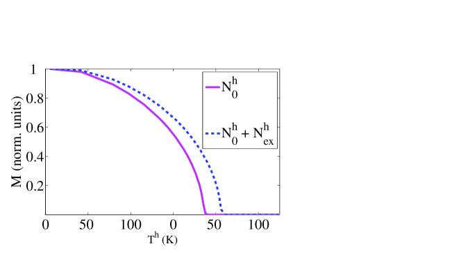
Figure 1: Temperature dependence of the normalized equilibrium ion magnetization for two hole densities. Here $N^{h}_{ex}=5\times 10^{19}\textrm{cm}^{-3}.$

In Fig. 1 we show the normalized equilibrium ion magnetization $\mathbf{M}/N^{M}$ as a function of the temperature and parameterized by the hole density $N^{h}$. In the figure, $N_{0}^{h}$ indicates the initial density of holes, $N_{ex}^{h}$ the excess of holes excited by the laser pulse, and $N^{h}=N_{0}^{h}+N_{ex}^{h}$. After the laser excitation, the magnetic impurities strongly interact with the out-of-equilibrium hole gas by means of the $\mathcal{H}_{pd}$ exchange interaction which redistributes the spin polarization from one system to another while conserving the total spin magnetization. Meanwhile, the itinerant hole spin is efficiently dissipated through spin-orbit interactions ($\tau_{SO}\approx 100$ fs) and relaxation of the total magnetization can be observed. Short-time spin relaxation of the holes is therefore an essential ingredient for explaining the observed time-dependent changes of the magnetization in ferromagnetic semiconductors Wang_05 ; Cywiski_07 .

By means of a standard relaxation model, we include both the spin-orbit mechanism (or any other mechanisms leading to the hole-spin relaxation) and the other thermalization effects, such as the cooling of the kinetic energy of the excited holes driven by the phonons, and the radiative recombination of the electron-hole pairs. The corresponding equations read as follow

$$\left.\frac{\partial n^{h}_{s}}{\partial t}\right|_{so} = \frac{n^{h}_{s}-\overline{n^{h}_{s}}}{\tau_{SO}}$$ (18)

$$\frac{\partial N^{h}}{\partial t} = \frac{N^{h}-N^{h}_{0}}{\tau_{RR}}$$ (19)

$$\frac{\partial T^{h}}{\partial t} = \frac{T^{h}-T^{L}}{\tau_{L}}$$ (20)

where $T^{h}(t)$ and $T^{L}$ are the temperatures of the holes and the lattice, $\overline{n^{h}_{s}}(n^{M}_{m},T^{h})$ is the self-consistent quasi-static equilibrium hole spin distribution computed from the Zener-type model of Kim_06 , which depends parametrically on the time-dependent ion magnetization $\mathbf{M}$. The temperature relaxation rate $\tau_{L}^{-1}=\tau_{OP}^{-1}+\tau_{AP}^{-1}$ takes into account both the acoustic phonon scattering with $\tau_{AP}=200$ ps and the optical phonon scattering with $\tau_{OP}=1$ ps for $T^{h}>50$ K and $\tau_{OP}=\infty$ for $T^{h}<50$ K Shah_book . Eq. (19) takes into account the radiative recombination process characterized by a relaxation time $\tau_{RR}=400$ ps Shah_book .

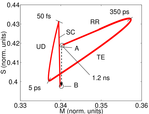
Figure 2: Evolution of the normalized holes magnetization ($\overline{S}$) and impurities magnetization ($\overline{M}$), in the $\overline{S}-\overline{M}$ plane, for $T^{L}=70$ K.

In Fig. 2 we present the time evolution of the normalized magnetizations, where the vertical axis corresponds to $\overline{S}=\mathbf{S}/N^{h}$ and the horizontal axis to $\overline{M}=\mathbf{M}/N^{M}$. In agreement with the experiment of Wang_07 , we consider a regime of small excitation (laser pump fluence of 1 $\mu$Jcm^-2) and a lattice temperature of $70$ K. The point A represents the initial spin polarization which is suddenly shifted (instantaneously in our model) to point B. This is due to the laser excitation which abruptly enhances the hole density and consequently changes the normalization of $\overline{S}$, so that $\overline{S}(0^{-})=\frac{\mathbf{S}(0^{-})}{N_{0}^{h}}$ and $\overline{S}(0^{+})=\frac{\mathbf{S}(0^{-})}{N^{h}}$. Our numerical simulations reveal the presence of different time evolution regimes: (i) $0<t<50$ fs: during this initial phase the magnetization evolution is nearly coherent (semi-coherent regime SC in Fig. 2). Indeed, since the photoexcited holes experience efficient spin-flip scattering with the localized Mn magnetic moments, a net spin polarization is transferred from the ion impurities to the holes leading to a significant increase of the hole spin polarization. Correspondingly, due to the large difference in densities between the two populations, only a small decrease of the ion magnetization is observed; (ii) 50 fs $<t<5$ ps: the nonequilibrium hole spin polarization is efficiently dissipated via the spin-orbit coupling, which leads to a net decrease of the total spin magnetization (see also Fig. 3). During this ultrafast demagnetization regime (UD) the kinetic temperature of the excited holes is still high; (iii) 5 ps $<t<350$ ps: the hole distribution loses its energy via carrier-phonon scattering and the hole temperature decreases over the time scale $\tau_{L}$. When the Curie temperature is reached, the holes and ions spins begin to align, which allows the system to recover a ferromagnetic order. Since the total number of holes relaxes to its initial value $N_{0}^{h}$ over a slower time scale $\tau_{RR}\gg\tau_{L}$, a ferromagnetic state with an excess of holes can be reached, thus justifying a transient enhancement of the total magnetization (TE regime); (iv) 350 ps $<t<1.2$ ns: finally the radiative recombination of the electron-hole pairs brings the system back to its initial configuration (RR regime).

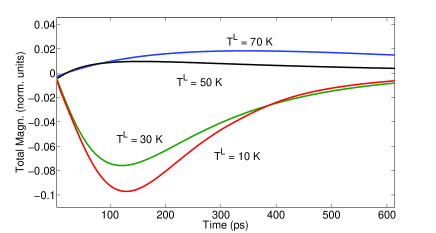
Figure 3: Time evolution of the total magnetization for different lattice temperatures: $T^{L}=10$ K (red line), $T^{L}=30$ K (green line), $T^{L}=50$ K (black line) and $T^{L}=70$ K (blue line).

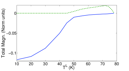
Figure 4: Minimum (solid line) and maximum (dashed line) of the total magnetization for different lattice temperatures.

The time evolution of the total magnetization for different lattice temperatures is depicted in Fig. 3. We see that the minimum of the total magnetization shifts to shorter times with increasing lattice temperature, in agreement with experimental findings. In Fig. 4 we plot the excursion of the total magnetization for different lattice temperature: only for $45$ K $<T^{L}<78$ K an enhancement of the total magnetization may be observed Wang_05 .

Finally, in order to validate the approximation of Eq. (13), we compare in Fig. 5 the time evolution of the total magnetization obtained by using either the approximate formula (14) or by evaluating numerically the integral of Eq. (13). As can be clearly seen, a good agreement is obtained, justifying the use of the simplified expressions (15) and (16).

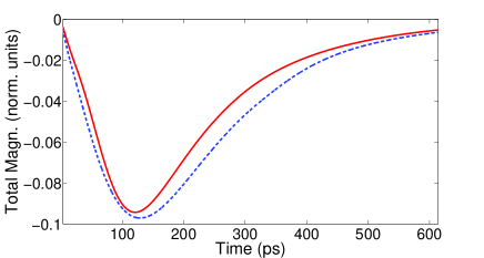
Figure 5: Time evolution of the total magnetization at $T^{L}=10$ K. Full line: exact formula, Eq. (13); dashed line: approximated formula, Eq. (14).

V Conclusion

In order to describe the strong spin-spin scattering regime observed in diluted magnetic semiconductors, we have derived a dynamical model that goes beyond the usual mean-field approximation. This model is based on the pseudo-fermion formalism and on a second-order many-particle expansion of the $p-d$ exchange interaction, which is performed in terms of the single-particle density functions. At this level of description, this approach is similar to that of Ref. Cywiski_07 , which was derived following a different perspective. Numerical simulations showed that our model is able to reproduce qualitatively – and to some extent quantitatively – the long-time evolution of the total magnetization after laser irradiation, as seen in recent experiments Wang_07 . The early demagnetization observed in the experiments is explained as the result of a net flow of polarization from the ions to the holes, which is subsequently dissipated via spin-orbit coupling. Thus, the typical demagnetization time scale is mainly determined by the nonlinear coupling between the ions and holes spins, with a lower bound given by the spin-orbit time scale, $\tau_{SO}\approx 100~{}\rm fs$. The demagnetization process cannot be faster than $\tau_{SO}$, but can be significantly slower, depending on the lattice temperature. In addition – and in contrast to Ref. Cywiski_07 – other slower processes (namely, holes thermalization and radiative recombination) were also included in the description, so that the global model encompasses time scales going from a few tens of femtoseconds to hundreds of picoseconds.

We point out that the methodology developed in this work can be naturally extended to higher orders by using perturbative field-theoretic techniques. In particular, we plan to investigate third order dynamical processes, which were neglected here but may play an important role in the regime of higher photoexcitation energy.

Finally, in the model used in this work only the heavy-hole band contribution to the exchange interaction was taken into account. The inclusion of a realistic band structure is currently under study.

Acknowledgements
We thank P. Gilliot and J.-Y. Bigot for useful discussions. This work was partially funded by the Agence Nationale de la Recherche, contract n. ANR-06-BLAN-0059.

References

(1) E. Beaurepaire, and J.-C. Merle, A. Daunois, and J.-Y. Bigot, Phys. Rev. Lett. 76, 4250 (1996).
(2)H. Ohno, Science 281, 951 (1998).
(3)T. Dietl, H. Ohno, F. Matsukura, J. Cibert, and D. Ferrand, Science 287, 1019 (2000).
(4)J. Wang, C. Sun, J. Kono, A. Oiwa, H. Munekata, Ł. Cywiński, and L. J. Sham, Phys. Rev. Lett. 95, 167401 (2005).
(5)C. Zener, Phys. Rev. 81, 440 (1951).
(6)B. Lee, T. Jungwirth, and A. H. MacDonald, Phys. Rev. B 61, 15606 (2000).
(7)N. Kim, H. Kim, J. W. Kim, S. J. Lee, and T. W. Kang, Phys. Rev. B 74, 155327 (2006).
(8)Y. Tserkovnyak, G. A. Fiete, and B. I. Halperin, Appl. Phys. Lett. 84, 5234 (2004).
(9)J. Wang, I. Cotoros, K. M. Dani, X. Liu, J. K. Furdyna, and D. S. Chemla, Phys. Rev. Lett. 98, 217401 (2007).
(10)B. König, I. A. Merkulov, D. R. Yakovlev, W. Ossau, S. M. Ryabchenko, M. Kutrowski, T. Wojtowicz, G. Karczewski, and J. Kossut, Phys. Rev. B 61, 16870 (2000).
(11) J. Chovan, E. G. Kavousanaki, and I. E.
Perakis, Phys. Rev. Lett. 96, 057402 (2006).
(12)Ł. Cywiński and L. J. Sham, Phys. Rev. B 76, 045205 (2007).
(13)J. Wang, Ł. Cywiński, C. Sun, J. Kono, H. Munekata, and L. J. Sham, Phys. Rev. B 77, 235308 (2008).
(14) A. A. Abrikosov, Physics 2, 5 (1965).
(15) P. Coleman, Phys. Rev. B 28, 5255 (1983).
(16)R. Winkler, Spin-Orbit Coupling Effects in Two-Dimensional Electron and Hole Systems,
Springer Tracts in Modern Physics (Springer, Berlin, 2003), Vol.
191.
(17) H. Haug and S. W. Koch, Quantum Theory of the optical and electric properties of
semiconductors (World Scientific, 1994).
(18)B. Koopmans, J. J. M. Ruigrok, F. Dalla Longa, and W. J. M. de Jonge, Phys. Rev. Lett. 95, 267207 (2005).
(19)J. Shah, Ultrafast Spectroscopy of Semiconductors and Semiconductor
Heterostructures (Springer, Berlin, 1999).