Optical polarisation of the Crab pulsar: precision measurements and comparison to the radio emission

Abstract

The linear polarisation of the Crab pulsar and its close environment was derived from observations with the high-speed photo-polarimeter OPTIMA at the 2.56-m Nordic Optical Telescope in the optical spectral range (400–750 nm). Time resolution as short as 11 $\mu$s, which corresponds to a phase interval of 1/3000 of the pulsar rotation, and high statistics allow the derivation of polarisation details never achieved before. The degree of optical polarisation and the position angle correlate in surprising details with the light curves at optical wavelengths and at radio frequencies of 610 and 1400 MHz. Our observations show that there exists a subtle connection between presumed non-coherent (optical) and coherent (radio) emissions. This finding supports previously detected correlations between the optical intensity of the Crab and the occurrence of giant radio pulses. Interpretation of our observations require more elaborate theoretical models than those currently available in the literature.

1 Introduction

Table 1: High energy polarisation measurements of pulsars and their nebulae. Polarisation degree is given as a percentage, and position angle in degrees (North, $0^{\circ}$ to East, $90^{\circ}$).

Band	Pulsar / Polarisation	Nebula (near PSR)	Ref.
	Crab
Optical (V$\sim 16.6$)	phase-resolved (Fig. 4)	$9.7\%\pm 0.1\%$ ; $139.8\degr\pm 0.2\degr$	[1], [2], [3]
	phase-averaged $9.8\%\pm 0.1\%$ and $109.5\degr\pm 0.2\degr$	($<5\arcsec$ from PSR)
UV	phased-resolved, similar to optical -		[4]
	P.D. and P.A. (MP and IP)
X-ray	only upper limits	$19.2\%\pm 0.9\%$; $155.8\degr\pm 1.4\degr$	[5], [6]
Hard X-ray/ soft $\gamma$-ray	off-pulse (phase: 0.52–0.88) $>72\%$; $120.6\degr\pm 8.5\degr$		[7]
	phase-averaged $47\%^{+19\%}_{-13\%}$; $100\degr\pm 11\degr$		[7]
$\gamma$-ray	off-pulse (phase: 0.5–0.8) $46\%\pm 10\%$; $123\degr\pm 11\degr$		[8]
	B0540-69
Optical (V$\sim 22.5$)	phase-averaged: $\sim 5\%$, no error quoted; phase-resolved: $<15\%$	$5.6\%\pm 1.0\%$ ; $79\degr\pm 5\degr$	[9], [10], [11]
	Vela
Optical (V$\sim 23.6$)	phase averaged: $9.4\%\pm 4\%$, $146\degr\pm 11\degr$		[9], [12]
	B0656+14
Optical (V$\sim 25$)	double peak light curve; P.D. bridge $\sim$ 100%, peaks $\sim$ 0%		[13]
	P.A. sweeps in agreement with RVM
	B1509-58
Optical (V$\sim 25.7$)	phase-averaged: $\sim 10.4\%$ (very uncertain, no error quoted)		[9]

[1] Smith et al. (1988), [2] Słowikowska et al. (2008), [3] this paper, [4] Graham-Smith et al. (1996), [5] Silver et al. (1978), [6] Weisskopf et al. (1978), [7] Forot et al. (2008), [8] Dean et al. (2008), [9] Wagner & Seifert (2000), [10] Middleditch et al. (1987), [11] Chanan & Helfand (1990), [12] Mignani et al. (2007), [13] Kern et al. (2003),

The Crab pulsar and its pulsar wind nebula (PWN) are two of the most intensively studied objects in the sky. The compact remnant of SN1054, a cornerstone of high energy astrophysics, is one of the youngest and most energetic pulsar and its pulsed emission has now been detected throughout the electromagnetic spectrum from about 10 MHz (Bridle, 1970) up to $>25$ GeV with some evidence ($3.4\sigma$) of pulsed emission above 60 GeV (Aliu et al., 2008). The PWN was measured even up to energies of $\sim 100$ TeV (Aharonian et al., 2004; Allen, 2007; Allen et al., 2007). The pulsar and its nebula are predominantly sources of non-thermal radiation (synchrotron, curvature and inverse Compton processes), which is indicated not only by the broad-band spectral continua but also by the strong polarisation of these emissions. The outstanding brightness of the Crab across the electromagnetic spectrum makes it the ideal target to investigate polarisation at all wavelengths where suitable instrumentation is available.

Before we focus on the Crab we want to introduce the subject of polarisation in pulsars by a short review of the total population: most pulsars were discovered in the radio regime (presently about two thousand objects are listed in the Australia Telescope National Facility Pulsar Catalogue, Manchester et al. 2005) and for for a large fraction of them polarisation studies were performed (e.g. Gould & Lyne, 1998; Karastergiou & Johnston, 2006). Most radio pulsars were found to show strong linear polarisation, including often a characteristic a swing of the position angle (P.A.) in an S-like shape near the pulse centre. This swing is interpreted in the ‘rotating vector model’ (hereafter: RVM, Radhakrishnan & Cooke, 1969) as a projection of the magnetic field line at the point of emission onto a plane perpendicular to the observer’s sight-line. The point of emission is usually assumed to be in the polar cap region of the pulsar where a regular dipolar field line points with a small angle (beam width) towards the observer. The free parameters of this simple geometrical model are the inclination angle between the axes of rotation and magnetic dipole, and the viewing angle between the line of sight and the rotation axis. Analyses of radio polarisation from many pulsars (e.g. references in Lyne & Graham-Smith, 2006) showed that most sources can be described in a polar cap model with an RVM and the intrinsic polarisation could be as high as $100\%$. Several pulsars however, especially at radio frequencies above several GHz, show reduced or complex polarisation signatures with indications of depolarisation or switching between modes of polarisation. These complications could arise from the subtle and often highly variable and unstable nature of the coherent processes underlying the radio emission.

The situation changes when going to higher energies, i.e. optical, X- and $\gamma$-ray regimes. Incoherent single particle radiation processes in the magnetosphere provide the high-energy pulsar emission (thermal emission from the neutron star surface is not considered here). Precise polarisation measurements of polarisation degree (P.D.) and P.A. as a function of pulsar phase in a wide range of energies should provide deep insight into the pulsars emission mechanisms, particle spectra, and emission site topologies. Fast X- and $\gamma$-ray polarimetry from space borne instruments is presently of very limited sensitivity. Therefore results have been reported only for the brightest pulsar and its PWN, i.e. the Crab. In the optical domain the situation is somewhat reversed: here the polarimeters are quite sensitive but the optical magnitudes of most pulsars are very faint. Therefore, despite the increasing number of optical pulsars (fourteen are known), only for five of them attempts to measure the pulsar and/or nebular polarisation were made. Table 1 summarises these efforts. For three pulsars phase-resolved measurements were performed; for the remaining two only phase-averaged results are available. Again the Crab, being the brightest object, is the exception with a multitude of optical polarisation measurements.

The scarcity of optical polarisation measurements, either in a phase averaged mode or with time resolution of the pulsar rotation, is clearly due to the large difference in magnitude going from the brightest pulsar, i.e. the Crab, to the next, B0540-69, which is $\sim 6$ magnitudes fainter. Therefore only for the Crab pulsar fully phase resolved polarisation measurements have been possible so far. The first optical phase-resolved linear polarisation observations of the Crab pulsar (Wampler et al., 1969; Cocke et al., 1970; Kristian et al., 1970) showed that the polarisation angle sweeps through each peak and the polarisation degree decreases and then increases within each pulse, reaching the minimum shortly after the pulse peak. These early observations were limited to the main pulse (MP) and inter pulse (IP) phase ranges only. Interpretation of the polarisation pattern behaviour has been made in terms of geometrical models (Wampler et al., 1969; Radhakrishnan & Cooke, 1969; Cocke et al., 1973; Ferguson, 1973; Ferguson et al., 1974), some of which offer the possibility of determining the magnetospheric location of the radiation source (e.g. Cocke et al., 1973; Ferguson et al., 1974).

For a long time it was thought that optical radiation of the Crab pulsar persisted only through both peaks, the MP and IP, and in the bridge region between them, but not in the phase range following the IP and preceding the MP. Several phase resolved imaging observations (Peterson et al., 1978; Percival et al., 1993; Golden et al., 2000) showed however that radiation persists throughout the whole pulsar rotation. They found that the minimum intensity, consistent with coming from an unresolved source at the pulsar position, occurs immediately before the start of the MP within a phase range of approximately 0.779 and 0.845. This level, often called the DC level of the Crab pulsar, has been variously determined with an intensity relative to the MP maximum of $3.6\%$ (Peterson et al., 1978), $<0.9\%$ (Percival et al., 1993), or $\sim 1\%$ (Golden et al., 2000).

After this discovery, the linear polarisation of optical radiation from the Crab pulsar was measured by Jones et al. (1981) and Smith et al. (1988). Both results confirmed the previous observations and additionally showed the polarisation characteristics during both off-pulse phase ranges (bridge and DC). However, for the DC phase range the results were not conclusive. The polarisation degree was at a level of 70% and $47\pm 10\%$ and the position angle was $\sim 118\degr$ and $\sim 130\degr$ for Jones et al. (1981) and Smith et al. (1988), respectively.

Weisskopf et al. (1978) measured the linear polarisation of the X-ray flux from the Crab nebula at energies of 2.6 keV and 5.2 keV, independent of any contribution from the pulsar. Within a field of view of $3\degr$ the X-rays are polarised at a level of $19.2\%-19.5\%$ and a P.A. of $156\degr-152\degr$. For the pulsar itself only upper limits could be derived (Silver et al., 1978). No evidence for an energy dependence of the X-ray polarisation was found. Close to the pulsar the nebular optical polarisation is quite uniform (at $\sim 9\%-11\%$) but the position angles change steadily with radial distance; $2\arcsec-3\arcsec$ from the pulsar the mean value is around $140\degr$ but beyond $5\arcsec$ the position angle exceeds $155\degr$ and it is very location-dependent (McLean et al., 1983). The X-ray results for the nebula are in good agreement with the optical polarisation measurements which yield a $19\%$ polarisation at $162\degr$ for the central region of the nebula within $0\aas@@fstack{\prime}486$ radius (Oort & Walraven, 1956). The similarity of the optical and X-ray results indicates that the polarisation is independent of energy over a broad spectral range. Recently $\gamma$-ray phase-averaged (off-pulse phase region, i.e. 0.5-0.8) polarisation measurements of the Crab nebula and pulsar were reported by Dean et al. (2008) for the energy range $100~{}\rm{kV}-1~{}\rm{MeV}$. The P.D. was found at $46\%\pm 10\%$ and the P.A. is $123\degr\pm 11\degr$, which indicates that this energetic radiation is dominated by emission from the inner nebula around the pulsar. This results has been recently confirmed by Forot et al. (2008) by using the IBIS instrument on board of the INTEGRAL telescope to obtain the linearly polarised emission for energies between $200-800~{}\rm{keV}$ and extend polarisation characteristics for pulses and bridge phases (Tab. 1).

We structure the paper as follows: firstly we describe our instrumentation (§2). In §3 and §4 the observations, data reduction methodology and measurements of polarimetric and photometric standards are described. In §5 we present the results of the Crab nebula and its pulsar. Also in §5 we show the pulsar polarisation characteristics after subtraction of an unpulsed component and discuss time alignment between optical and radio wavelengths. In §6 we present a discussion of theoretical models and compare them to our measurements and end with a summary and conclusions.

2 Instrumentation

Our goal was to obtain polarisation characteristics of the Crab pulsar with very high time resolution as a function of the pulsar rotational phase. We used the 2.56-m Nordic Optical Telescope (NOT) for these measurements. This facility not only provides a mirror with reasonably large collecting area but also has an excellent performance in offset guidance and telescope control, which is important for instruments with very small entrance apertures. Moreover, contrary to many larger optical telescopes, guest instruments can be used at NOT. For the Crab pulsar observations carried out during November, 23–27 2003, we used the high-speed photo-polarimeter OPTIMA (Optical Pulsar TIMing Analyser). We shortly describe the system below. An extended description of the OPTIMA instrument is presented by Kanbach et al. (2003, 2008).

2.1 OPTIMA

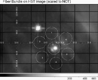
Figure 1: An enlargement of the HST image of the inner Crab nebula . North is up; East is left. The pulsar is identified with the lower/right of the two stars near the geometric centre of the nebula. A small arc-like feature (the inner knot) which is clearly resolved in the HST image is located $0\aas@@fstack{\prime\prime}65$ to the SE of the pulsar. The OPTIMA fibre bundle, centred on the pulsar and scaled with the NOT focal plane scale, is over plotted.

The basic requirement for a high-speed photometer is to select and time tag individual photons from a celestial source with high efficiency and precision. In the case of OPTIMA, which was primarily designed for studying the optical light curves of faint pulsars and other highly variable targets, the source flux is isolated in the focal plane of the telescope by the use of an optical fibre pick-up which acts as a diaphragm. The target fibre is central to a hexagonal bundle of identical fibres which measure the sky background and, in the case of the Crab nebula, the close environment of the pulsar (Fig. 1). OPTIMA uses commercial single photon counting modules with Avalanche Photodiodes (APDs). These APD counters have quantum efficiencies peaking at 70% for $\lambda\sim 700$ nm and a wide range with Q.E. $>20\%$ from 440 to 980 nm.

The light from the telescope at the Cassegrain focus is incident on a slant mirror with an embedded bundle of optical fibres. Optionally one can insert filters or a rotating linear polariser into the incoming beam. The field around the fibres, visible in the mirror (typical size $2\arcmin\times 3\arcmin$), is imaged with a target acquisition camera (type AP6, from Apogee Instruments). We use the following nomenclature for the fibre channels: channel 0 for the central fibre, channels 1 to 6 for the ring fibres and channel 7 for a sky background fibre, located about $1\arcmin$ off-set from the target fibre. For the observations we used tapered fibres with $320~{}\rm{\mu m}$ diameter at the pick-up and an exit diameter at the detector of $100~{}\rm{\mu m}$. The single fibre size in the focal plane is equivalent to a $2\aas@@fstack{\prime\prime}344$ resolution at the 2.56-m NOT telescope. Although the pure silica core fibres transmit light from 400 nm to $\sim$950 nm with better than $99\%$, the net transmission of the tapered fibres is lower and appears to range between $60\%$ and $90\%$.

The timing of individual photons is controlled by signals from the Global Positioning System (GPS) to an absolute accuracy of $\sim 2~{}\rm{\mu s}$, although the readout system limits the resolution to $\sim 4~{}\rm{\mu s}$. The OPTIMA detector is operated with two PCs and is autonomous except for the need to have a good telescope guiding system.

2.2 Rotating Polarisation Filter

For the present observations OPTIMA was equipped with a rotating polarisation filter (RPF) in the incoming beam above the fibre pick-up so that all fibre channels and the CCD image are fully covered. The polarising filter (Type 10K by Spindler & Hoyer) is mounted on a precision roller bearing and is rotated with typical frequencies of a few Hz (the averaged frequency over the whole observations was 3.4 Hz). Incoming linearly polarised light is then modulated at twice the rotation frequency of the filter. The reference position of the filter is given by a signal from a magnetic switch (Hall sensor) which is registered and timed in the same way as a photon event and stored in a separate DAQ channel. The position of the polarising filter for any photon event is then derived by interpolating the photon arrival time between the preceding and the following Hall sensor signal, i.e.:

$$\alpha_{\rm RPF}(TOA)=\frac{t_{TOA}-t_{b}}{t_{a}-t_{b}}\times 360\degr,$$

where $\alpha_{\rm RPF}(TOA)$ is the RPF angle at which the event was observed, $t_{TOA}$ is the event time of arrival, and $t_{b}$ and $t_{a}$ are the recorded times of the Hall signal sensor before and after $t_{TOA}$. Since, during one turn of the RPF all possible polarisation angles are measured two times, for all values bigger than $180\degr$ exactly $180\degr$ was subtracted.

Slight irregularities in the rotation frequency of the RPF that occur on time-scales longer than fractions of a second, e.g. due to supply voltage drifts or mechanical resistance changes in the bearing and motor, can thus be corrected with sufficient accuracy. The RPF was tested in the lab with unpolarised and linearly polarised light to ensure and prove that the OPTIMA fibres and detectors have no intrinsic systematic response to polarised light (Kellner, 2002).

The polarising filter modulates the incoming light effectively only over a wavelength range of about 470-750 nm. Since the APD response (QE$>20\%$) extends from about 450 nm to 970 nm and no wavelength information of the individual recorded events is available, it is necessary to block radiation outside the filter modulation range. Such photons, especially towards the near IR, are not modulated and would decrease the estimate for the degree of polarisation. Therefore, we inserted an IR blocking filter that cuts the wavelength range at about 750 nm.

The method to derive the polarisation characteristics follows the approach described by Sparks & Axon (1999). Details are given in Appendix A to this paper.

3 Observations

The Crab observations were performed on November 23–27 2003 (52966 – 52971 MJD). They consists of 160 pointings of ten minutes each. About one third of the total number of counts falls in the central fibre, whereas around 5 to 10 percent are registered in each of the background fibre (channels marked from 1 to 6 in the Fig. 1). The count rate for the central fibre decreases when the seeing deteriorates and photons spill out into the ring channels ($1\div 6$). In order to screen for observation intervals of acceptable seeing we therefore apply a cut on the fraction of total counts in channel 0 at the level of $30\%$. After screening for good seeing and proper pointing, our data base resulted in 83 files, equivalent to 13 hours and 43 minutes of total exposure.

4 Data reduction

4.1 Flat field correction

Table 2: Fibre flat field correction factors

Channel	Factor
0	$1.000\pm 0.012$
1	$1.009\pm 0.013$
2	$1.074\pm 0.013$
3	$0.899\pm 0.012$
4	$0.850\pm 0.011$
5	$0.956\pm 0.012$
6	$1.140\pm 0.014$

For flat field correction factors of all channels we used two sets of dark sky observations, i.e. pointing at $\alpha=00^{h}07^{m}02\aas@@fstack{s}00$, $\delta=+73\degr 03\arcmin 28\aas@@fstack{\prime\prime}00$. Both observations were taken on November 25. The data acquisition started at 21:39:10 UTC and 21:49:13 UTC. The exposure time amounted to 600 and 300 seconds for the first and second observation, respectively. The detected count rates behind the filters fluctuated from 180 Hz for channel 4 up to 240 Hz for channel 6. To obtain the flat field correction factors we assumed that this value was 1.0 for the central fibre, and we scaled the count rates of the other fibres to the central one. We binned the data in ten seconds intervals, and then calculated the average and standard deviation for each single channel of the ring fibres. The resulting numbers are shown in Tab. 2.

4.2 The HST polarisation standards

Table 3: HST polarisation and photometric standards chosen from the list of Turnshek et al. (1990)

Name /	Coordinates FK5	Comments
Spectral Type
HST Polarisation Standards
BD+64 106	$~{}00^{h}~{}57^{m}~{}36\aas@@fstack{s}70$	V = 10.34
B1V	$+64\degr~{}51\arcmin~{}34\aas@@fstack{\prime\prime}9$	$p=5.65\%\pm 0.053\%$
		$\theta$ = $96\aas@@fstack{\circ}8$
G191B2B	$~{}05^{h}~{}05^{m}~{}30\aas@@fstack{s}61$	V = 11.79
WD	$+52\degr~{}49\arcmin~{}51\aas@@fstack{\prime\prime}9$	$p=0.09\%\pm 0.048\%$
HST Photometric Standard
GD50	$~{}03^{h}~{}48^{m}~{}50\aas@@fstack{s}20$	V = 14.06
WD	$-00\degr~{}58\arcmin~{}31\aas@@fstack{\prime\prime}2$

Table 4: Measurements of the HST polarisation standard BD+64 104. Date and time of observations, as well as exposure length in seconds are given in the first, second and third row, respectively. Obtained values of P.D., $p$, (upper value) and P.A. ($\theta$, bottom value) are given for each OPTIMA detector channel from 0 to 6 ($p$ and $\theta$ are in percent and degrees, respectively). Additionally, last row (assigned as ‘$1\div 6$’ ) gives $p$ and $\theta$ values obtained after averaging the Stokes parameters from all ring channels. Mean gives $p$ and $\theta$, as well as their standard deviations, after averaging all existing data of BD+64 104. The obtained position angle of BD+64 104 (bold faced text in the row of channel 0) was later used for the OPTIMA instrument calibration.

BD+64 104
Obs. Date		25 Nov 2003			27 Nov 2003				Mean
Time [UTC]		22:07:01	22:09:46		21:33:35	21:36:08	21:38:34
Expo. [s]		140	130		110	120	120
Channel
0		1.30	1.35		1.98	1.86	1.67		$1.63\pm 0.30$
		96.6	96.8		96.2	96.9	97.2		96.74$\pm$0.37
1		4.57	4.64		3.71	3.60	4.21		$4.15\pm 0.48$
		100.3	96.6		98.0	96.5	98.3		$98.14\pm 1.62$
2		5.16	5.17		4.59	4.84	5.57		$5.07\pm 0.37$
		96.0	94.7		98.0	96.8	96.8		$96.46\pm 1.22$
3		5.38	5.16		5.49	5.08	5.04		$5.23\pm 0.20$
		94.3	92.9		95.5	95.9	97.4		$95.20\pm 1.70$
4		4.67	4.34		4.14	4.98	4.27		$4.48\pm 0.34$
		99.1	98.6		98.5	100.5	103.5		$100.04\pm 2.09$
5		5.51	5.26		5.53	5.58	5.38		$5.45\pm 0.13$
		96.7	94.3		97.9	96.2	97.1		$96.44\pm 1.35$
6		4.62	5.00		5.06	4.52	4.80		$4.80\pm 0.23$
		98.6	98.7		93.6	93.6	91.7		$95.24\pm 3.21$
1$\div$6		5.06	4.95		4.47	4.37	4.73		$4.72\pm 0.30$
		96.7	95.1		96.8	95.8	96.4		$96.16\pm 0.71$

Table 5: Measurements of the HST polarisation standard G191B2B and the HST photometric standard GD50. Date and time of observations, as well as exposure length in seconds are given in the first, second and third row, respectively. Obtained values of P.D., $p$, are given in percent for each OPTIMA detector channel from 0 to 6. Additionally, last row (assigned as ‘$1\div 6$’) gives $p$ values obtained after averaging the Stokes parameters from all ring channels. Mean gives $p$ and standard deviations after averaging all existing data of G191B2B from Nov 26th. In the last column the results of GD50 measurements are given.

G191B2B										GD50
Obs. Date		26 Nov 2003					Mean			27 Nov 2003
Time [UTC]		21:33:08	21:36:22	21:41:01	21:43:53					21:52:17
Expo. [s]		160	150	130	130					590
Channel
0		0.04	0.07	0.03	0.06		0.05 $\pm$ 0.02			0.08
1		0.37	0.48	0.47	0.21		0.38 $\pm$ 0.13			0.30
2		0.75	0.41	0.65	0.85		0.67 $\pm$ 0.19			0.44
3		0.84	0.46	0.80	0.72		0.71 $\pm$ 0.17			0.61
4		0.30	0.66	0.69	0.47		0.53 $\pm$ 0.18			0.62
5		0.16	0.56	0.36	0.16		0.31 $\pm$ 0.19			0.23
6		0.14	0.21	0.04	0.42		0.20 $\pm$ 0.16			0.53
1$\div$6		0.35	0.34	0.30	0.32		0.33 $\pm$ 0.02			0.22

We performed observations of stars with well known polarisation in order to understand the intrinsic polarisation and the response of the instrument. Since OPTIMA is very sensitive and limited in its capacity for data acquisition at high rates (count rates above 37 kHz lead to noticeable, but correctable, pile-up effects, Mühlegger 2006) we selected three of the weakest stars from the list of Turnshek et al. (1990); two polarisation and one photometric standards (Tab. 3). The first star of the two polarisation standards is highly polarised, on the level of $6\%$, whereas the second one has a very low polarisation degree of $\sim$1 ‰. Unfortunately for our measurements both of them are quite bright by OPTIMA standards. Therefore, we additionally performed optical polarisation measurements of a dimmer star, i.e. a photometric standard from Turnshek et al. (1990) list, expecting its light not to be polarised.

We observed the HST polarisation standard BD+64 106 for 270 and 350 seconds on the 25th and 27th of November, respectively (Tab. 4). The observing conditions during the two exposures were very different, requiring a detailed discussion of the results. On Nov 25, 22:06 - 22:12 UTC the average seeing was on the level of $1\aas@@fstack{\prime\prime}27$ (RoboDIMM measurements), whereas for the time span 21:33 - 21:40 UTC on Nov 27 no information about the seeing conditions was available from the RoboDIMM telescope. At the beginning of this night the weather was very good. But later, during less than two hours, between 20:00 and 22:00 hours, the humidity changed from 20% to almost 60%, and the wind speed increased up to 15 m/s. Therefore, the seeing on Nov 27 was probably worse than during Nov 25, likely more than $2\aas@@fstack{\prime\prime}0$. This difference in seeing causes different count rates in the central and ring fibres. On 25 Nov the count rate in channel 0 was about 190 kHz, and in the ring fibres $\approx 20~{}\rm{kHz}$, while during Nov 27 we had 150 kHz (centre) and $\approx 50~{}\rm{kHz}$ (ring). As a consequence of the high count rates ($\gg 37~{}\rm{kHz}$) the central channel was severely affected by pile-up in these observations. For the second set of data (27 Nov) it happened that some of the ring fibres, especially channels 1 and 6, were also saturated. The values of the polarisation degree and the position angle for all channels and for all sets of observations are gathered in Tab. 4. It is important to notice that, even if the central fibre was suffering pile-up, the calculated position angle for each single observation of BD+64 104 is very much constant. This is caused by the fact that the position angle, being the phase of the maximum of the modulated incoming light, is not strongly dependent on the pile-up effect. Saturation is however important when the amplitude of RPF modulation, corresponding to the degree of polarisation, is to be measured. We can observe this by comparing results in Tab. 4. For the central fibre there is significant difference in the polarisation degree for the first and second data set. When the dispersion of the stellar image due to seeing was larger the star light was more smoothly distributed among all channels, therefore an increase of $p$ in the central fibre is observed. Seeing conditions, being equivalent to the count rates in the ring, did not affect significantly the measured values of $p$ in the ring fibres. Only in the case of channel 1 the polarisation degree is much smaller during the Nov 27 observations than Nov 25. This is strongly connected with the fact that, during the second observation, this channel, among all of the ring channels, was the most saturated one.

Taking into account the resulting $\theta$ and $p$ (Tab. 4) of the HST polarisation standard BD+64 104 (being a very bright star as for the OPTIMA instrument) we can conclude that for the purpose of calibrating the north direction of our instrument it is safe and valid to use values of the polarisation angle from the central fibre (Tab. 4, bold faced text). The averaged value of $\theta_{\rm{BD+64104}}$ amounts to $96.74\degr\pm 0.37\degr$. This result was obtained by shifting the intrinsic RPF angles (the position of the Hall sensor indicates the origin of the intrinsic angles) by $92\degr$. The angles $\theta$ given here and hereafter in the text and tables are the $E-$vector position angles relative to celestial north (N to E). Due to the pile-up in the central fibre the best estimate of the polarisation degree of BD+64 104 comes from the sum of the light detected in the ring fibres. The obtained value, $4.72\%\pm 0.30\%$, is somewhat smaller than the value given by Turnshek et al. (1990), $5.65\%\pm 0.053\%$, but one should take into account the systematic problems encountered with such a bright standard star. In this case the bad seeing (high value) is an advantage, because it naturally defocuses our target. We also performed observations of the unpolarised HST standard G191B2B (Tab. 3 and 5). Data for this target were taken on 26 Nov, 21:33 UTC for about 10 minutes with seeing being on the level of $1\aas@@fstack{\prime\prime}0$. We found a very small polarisation degree for this star, as expected, and thus the position angle has little meaning. During these observations the count rate was on the level of 150 kHz and $\la 40~{}\rm{kHz}$ in the central and ring fibres, respectively. We should point out that channel 0 was affected by pile-up and the result $0.05\%\pm 0.02\%$ (Tab. 5) might be biased, even if it is in good agreement with the value $0.09\%\pm 0.048\%$ given by Turnshek et al. (1990). The averaged value of P.D. from the background fibres is higher. It amounts to $0.33\%\pm 0.02\%$, and is probably partly contaminated by the polarised sky background.

For the purpose of the instrument calibration we also chose from the Turnshek et al. (1990) atlas of HST photometric, spectroscopic, and polarimetric calibration objects a star with brightness that should assure count rates lower that the pile-up threshold, i.e. GD50 (Tab. 3). It is a photometric standard, thus we expect its light not to be polarised. Observations of this target were performed on Nov 27th at 21:52 UTC with recorded count rates in the central channel of 10-15 kHz and in the ring channels $\la 1~{}\rm{kHz}$. Results are shown in the Tab. 5. The source had polarisation degree below 1‰ (measured in the central fibre), whereas the measured $p$ within the ring fibres was about three time greater. These values correspond to the sky background polarisation. However, the sky background could have been more highly polarised. The contribution of the night sky to the observed count rates was on the level of one quarter in each fibre only, i.e. the background ring fibres were contaminated by the source. Thus, the signal measured in the ring fibres was most probably depolarised and could have higher polarisation degree in reality.

4.3 Raw data binning for the Crab analysis

Table 6: The Crab pulsar radio ephemeris

Parameter	Value
R.A. (J2000), $\alpha_{2000}$	$05^{h}34^{m}31\aas@@fstack{s}972$
DEC (J2000), $\delta_{2000}$	$+22\degr 00\arcmin 52\aas@@fstack{\prime\prime}07$
Valid range (MJD)	52944–52975
Epoch, $t_{0}$ (TDB MJD)	52960.000000296
$\nu_{0}$ (Hz)	29.8003951530036
$\dot{\nu_{0}}~{}\rm{(10^{-10}~{}Hz~{}s^{-1})}$	-3.73414
$\ddot{\nu_{0}}~{}\rm{(10^{-20}~{}Hz~{}s^{-2})}$	1.18

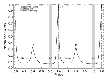
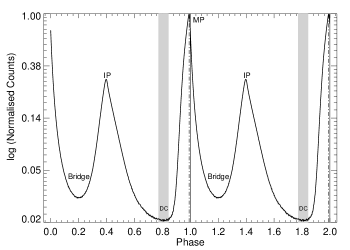
Figure 2: The Crab pulsar light curve obtained from photons recorded by the OPTIMA central fibre APD (channel 0). The components of the light curve are indicated as follows: main pulse MP, inter pulse IP, non-zero intensity level between MP and IP, i.e. bridge, as well as the DC region, previously known as the ‘off-pulse’ component in in the phase range $0.7729-0.8446$ . The upper panel shows the raw light curve including counts from the nebula and the sky background. In the lower panel the lightcurve is shown in a logarithmic scale after subtraction of the nebular and sky backgrounds. This display shows clearly the DC intensity level. Two rotation periods are shown for clarity.

For each incoming and detected photon the OPTIMA data acquisition system stores its Time Of Arrival (TOA) in a compact proprietary binary format with a resolution of $4~{}\rm{\mu s}$. By using the OPTIMA system software (Straubmeier, 2001) one can obtain TOAs in units of Julian Date (JD). In order to apply the rotational model of the pulsar derived from radio observations to our optical photons, it is required to measure the TOAs in an ‘inertial observer frame’. Using the NOT position coordinates, the Crab pulsar coordinates (Tab. 6) and as planetary ephemeris the JPL DE200 tabulations (Standish, 1982) we transformed the recorded TOAs to the commonly used, and (for these purposes) inertial frame, i.e. to TOAs at the solar system barycentre.

Parameters of the rotational model of the Crab pulsar (Tab. 6) obtained from the radio observations are regularly, once per month, published by the Jodrell Bank Observatory pulsar group in the Crab Pulsar Monthly Ephemeris (Lyne et al., 1993). For each recorded event (TOA) the corresponding pulsar phase and the phase of the RPF is calculated. We sort the individual events into a 3D data array. The first dimension is given by the rotational phase of the pulsar (binned with various resolutions), the second one by the phase of the polarisation filter at each photon TOA (binned in $1\degr$ intervals), and the third dimension is the fibre number or number of DAQ channels (seven channels).

To obtain an ’unpolarised’ light curve, e.g. with a time resolution of $67~{}\rm{\mu s}$ which assures a good S/N ratio even for the phase ranges where the intensity is very low, the data array is constructed with 500 bins per rotational period of the Crab, and the events spread out over the RPF phases are all added up. The Crab light curve, in its raw form as the measured count rate in the central fibre without background subtraction, is shown in the top panel of Fig. 2. We indicate the components main pulse (MP), inter pulse (IP), non-zero intensity level between two peaks - bridge, and the DC region, previously known as the so called ‘off-pulse’ component. For our further analysis we define the DC component as the counts between phases $0.7729-0.846$, which is in accordance with the findings of Percival et al. (1993). The same light curve after background subtraction (method described in the next section) is shown in the lower panel of Fig. 2 with a logarithmic scaling to enhance the visibility of the DC level. The higher S/N ratio in the peaks allows us to use better time resolution for these phase ranges, i.e. up to 3000 bins per period, which corresponds to a bin of 11 $\mu s$ interval (Figs. 4, 5, 6).

5 Results for the Crab nebula and pulsar

5.1 Nebular contribution

Table 7: The Crab nebula’s P.D. and P.A. at the DC phase range

Channel	$p$ [%]	$\theta$ [$\degr$]
0	33.08(25)	118.8(0.2)
1	9.05(8)	141.3(2)
2	10.30(8)	142.5(2)
3	8.77(7)	148.4(2)
4	9.35(8)	136.6(2)
5	11.50(8)	133.1(2)
6	10.26(7)	137.9(2)
1$\div$6	9.71(8)	139.8(2)

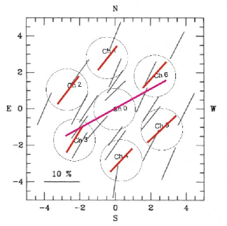
Figure 3: Polarisation of the Crab nebula as measured by each single fibre at the minimum phase of the pulsar light curve. It is graphic representation of results given in Tab. 7. The axes are calibrated in arc seconds centred on the pulsar. The scaled OPTIMA fibre bundle is over plotted on the figure given in Smith et al. 1988. The aperture of a single fibre is $2\aas@@fstack{\prime\prime}35$. The pink line for central fibre and the red lines for the ring fibres represent our measurements with the rotating polaroid filter. The black lines are the results that Smith et al. 1988 determined with a polarimeter based on a rotating half-wave plate and a Foster prism.

The Crab synchrotron nebula is a relativistic magnetised plasma that is powered by the spin-down energy of the pulsar. It was the first recognised astronomical source of synchrotron radiation. The synchrotron nature of the radiation was confirmed by optical polarisation observations (Woltjer, 1957). The conversion efficiency of the nebula is quite high, with 10%–20% of the spin-down energy released by the pulsar appearing as synchrotron radiation. The inner synchrotron nebula is a region consisting of jets, a torus of X-ray emission, small-scale variations in polarisation and spectral index, and complexes of sharp wisps. Most theoretical models associate the sharp wisps seen at visible and radio wavelengths with the location of the shock wave between the pulsar and the synchrotron nebula. Closer to the outer boundary of the nebula are the filaments - the chemically enriched material ejected during the supernova explosion observed by Chinese astronomers in 1054.

For a long time the imaging investigations of the Crab nebula were limited in a fundamental way by the spatial resolution of the detectors, not being able to reveal a wealth of subarcseconds structures. A breakthrough in the optical studies of the structure of the Crab nebula was undertaken by using the Wide Field and Planetary Camera 2 (WFPC2) on board of the Hubble Space Telescope. Hester et al. (1995) performed this observation with $0\aas@@fstack{\prime\prime}1$ resolution. Below we shortly describe the most important HST results that are important in the context of this paper.

They discovered a bright knot of visible emission located $0\aas@@fstack{\prime\prime}65$ to the south-east of the pulsar, along the axis of the system (Fig. 1). This inner knot, along with a second similarly sharp but fainter knot (hereafter outer knot) located at a distance of $3\aas@@fstack{\prime\prime}8$ from the pulsar, lies at an approximate position angle of $\sim 115\degr$ east to north. Both knots are aligned with the X-ray and optical jet to the south-east of the pulsar and are elongated in the dimension roughly perpendicular to the jet direction, with lengths of about a half arc second. Both, the inner and outer knot appear to be present but not well resolved in the images of the Crab nebula previously taken by ground based telescopes. Fig. 1 is an enlargement of the co-added HST WFPC2 images of 12 observations of the Crab nebula in between 2000 and 2001 with the F547M filter (observations group index 6 of Ng & Romani, 2006, it was kindly supplied by Roger Romani, private communication). The pulsar is identified with the lower/right of the two stars near the geometric centre of the nebula. The OPTIMA fibre bundle centred on the pulsar and scaled with the NOT focal plane scale is over plotted. It is clear that we are not able to resolve the Crab pulsar from the inner knot within the central fibre. Moreover, with seeing being bigger than $1\aas@@fstack{\prime\prime}0$ the pulsar light is somewhat spread into the ring channels. Evidence of this effect is seen in the light curves when the intensities measured by individual ring fibres are folded with the pulsar phase and pulsed emission is detected. Additionally, there may be contributions of photons coming from the outer knot (not very clearly seen in the Fig. 1), but an indication of it can be seen on the south-east side in between the fibres 3 and 4. It is also noteworthy to mention that the ring fibres see different patches of nebulosity. One third of all counts are recorded in the central fibre. The background fibres contribute to the total number of counts in the percentage of 9, 10, 14, 11, 12, 11 for channels from 1 to 6, respectively.

To obtain the polarisation characteristics of the pulsar neighbourhood we assumed that within the DC phase range the contribution of the pulsar emission to the ring fibres is minimal. The integrated pulsed contribution in each fibre (spill-out from the pulsar) with respect to the total counts in the fibre is on the level of $3.1\%$, $4.5\%$, $4.4\%$, $2.5\%$, $2\%$, $1.9\%$ for the channels from 1 to 6, respectively. Therefore, during our background (nebula) calculations we consider only light coming within the ‘off-pulse’ phase range, i.e. 7% of the whole rotational cycle of the Crab pulsar. Obtained polarisation degree and position angles for each of the single OPTIMA apertures are given in Tab. 7, as well as illustrated in the Fig. 3. We compared our results with previous ones by over plotting them on the polarisation sky map of the very close neighbourhood presented by Smith et al. (1988). By averaging the Stokes parameters over all background channels we get $p=9.71\%\pm 0.08\%$ and $\theta=139.8\degr\pm 0.2\degr$ for the region surrounding the pulsar. Close to the pulsar the nebular polarisation is quite uniform ($\sim 9-11\%$) but the position angles change steadily with radial distance. Two to three arc seconds from the pulsar the mean value is around $140\degr$ but beyond five arc seconds the position angle exceeds $155\degr$ and it is very position-dependent (McLean et al., 1983).

5.2 Polarisation characteristics of the Crab pulsar

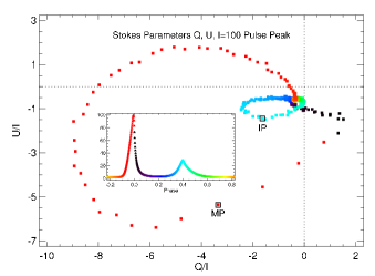
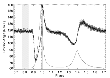
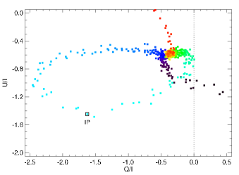
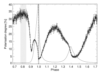
Figure 4: Left column: Stokes parameters $Q$, $U$ as a vector diagram. Colours refer to the pulse phases as indicated in the input box of upper panel. The scale is such that $I=100$ at the maximum light. Phases of the MP and IP maxima are indicated with black open squares. Points belonging to the MP and IP follow in a counter-clockwise direction on outer and inner ellipses, respectively. Bottom panel shows a zoomed region around the IP phases. The dashed lines indicate the origin of the scaled Q,U coordinates. Any error in background polarisation would correspond to a shift in the origin in this plot. The lower plot shows an zoomed region of the upper panel. Right column: The Crab pulsar position angle as a function of rotational phase (upper panel). Changes of $\theta$ are aligned with the MP maximum of the optical light (vertical dot-dashed line), but also with the zero phase, i.e. with the radio phase of the MP (vertical solid line, see Fig. 5 for details). The Crab pulsar polarisation degree as a function of rotational phase (bottom panel). Minimum of $p$ is for the radio phase (vertical solid line), and not for the maximum phase of the optical MP (vertical dot-dashed line, see Fig. 5 for details). For both panels a bit more than one rotation is shown for clarity. The pulse profile (solid line) and DC phase range (dashed region) are indicated also. The DC component in the phase range 0.78–0.84 has P.A. $\sim 119\degr$, and P.D. $\sim 33\%$. One sigma errors are show.

Figure 5: Polarization characteristics of the Crab pulsar - P.A. (top row) and P.D. (bottom row) - as a function of rotational phase. Data binning is 1000 and 3000 bins per cycle (corresponding to $33.5~{}\rm\mu s$ and $11~{}\rm\mu s$ per bin) for odd and even columns, respectively. The first two columns are zoomed around the MP phase (using different scales), whereas the next two are zoomed around the IP phase. Dot-dashed vertical line indicates the optical MP maximum phase (=0.993), as well as the IP maximum phase (= 1.398). Solid vertical line indicates the radio peak phase (=1.0). For clarity the optical light curve of the Crab pulsar is over plotted (solid line).

The Crab pulsar is detected at all phases of rotation, i.e. also in the so-called ‘off-pulse’ phase with an intensity of about 2% compared to the maximum intensity of the main pulse. As mentioned before, the measured level of the DC differs from author to author. For example very early measurements performed by Peterson et al. (1978) gives the ‘unpulsed background’ from the Crab pulsar on the level of 3.6% of the main peak intensity. Much lower values were obtained by Jones et al. (1981) and later by Smith et al. (1988): 0.6% and 1.2%, respectively. In addition Percival et al. (1993) claims that the ‘off-pulsed’ flux has an intensity less than 0.9% of the peak flux (visible and UV data from $HST$, $2\sigma$ upper limit), whereas a fractional flux derived by Golden et al. (2000) from photometric analysis gives $\sim 1\%$.

For the background (nebula and sky) subtraction we took the averaged Stokes parameters ($I_{DC},{Q_{DC}},U_{DC}$) recorded in the ring fibres over the ‘off-pulse’ phase. The pulsar Stokes parameters ($I$, $Q$, $U$; Fig. 11) as a function of its rotational phase are derived after subtracting from the central channel measurements the steady nebular component. The colour coded Stokes parameters $Q$, $U$ as a vector diagram are shown in the Fig. 4. Colours refer to the pulse phases as indicated in the input box and the scale is such that $I=100$ at the maximum light, i.e maximum of the MP. The MP and IP maxima are indicated with black open squares. Points belonging to the MP phases follow an outer ellipse (upper panel), whereas these belonging to the IP an inner one (bottom panel). In both cases the direction of increasing pulsar phase is counter-clockwise. Noteworthy is that already from the Stokes parameters one can see that there is sudden change in the pattern near the radio phase, i.e. where the red points change to the black ones. As the next step of the data analysis the polarisation characteristics, the position angle and the degree of polarisation of the E-vector, are calculated from the Stokes parameters (Q. 2). Results plotted with a different time resolution are presented in Fig. 4 and Fig. 5.

Optical emission from the Crab pulsar is highly polarised, especially in the bridge and the ‘off-pulse’ phases. The position angle and the degree of linear polarisation as functions of rotation phase show well determined properties:

• The polarisation characteristics of both, the MP and the IP components, are quite similar.

• The polarisation degree reaches a minimum at phase close to the radio main peak; the minimum is not aligned with the optical peak.

• There is a well defined bump in the polarisation degree on the rising flank of the MP.

• There is an indication of such a bump also for the IP (especially after DC subtraction).

• The position angle swings through a large angle in both peaks: after subtraction of the DC component the angle swing is 130$\degr$ and 100$\degr$ for MP and IP, respectively.

• The position angle at the bridge and ‘off-pulse’ phases is constant.

• The position angle slope changes dramatically at phases 0.993 (MP maximum) and 1.0 (radio peak).

• The trailing wing of the MP (phase range 1.0-1.03) shows a linearly increasing degree of polarisation. This feature turns into a bump shape after DC subtraction. There is a slight indication of the same behaviour for the trailing wing of the IP.

5.3 Polarisation characteristics of the Crab pulsar after DC subtraction

Figure 6: The same as in Fig. 5 but after DC subtraction.

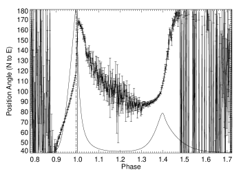
Figure 7: The same as Fig. 4 but after DC subtraction.

The apparent constancy of the position angle within the phase range 0.78–0.84 (Fig. 4, right upper panel) may suggest that the optical emission from the Crab pulsar consists of two components - pulsed and unpulsed. The pulsed component is characterised by a highly variable position angle and polarisation degree. The unpulsed (i.e. DC) component is characterised by constant intensity on the level of 2% of the main pulse intensity, fixed $\theta\sim 119\degr$, and a degree of polarisation on the level of 33%. The source of emission of the DC is unknown. There are various ideas from where in the magnetosphere or the nebula this component might arise. It is also possible that the inner knot (located only $0\aas@@fstack{\prime\prime}65$ apart from the pulsar and being a persistent feature throughout the sequences of the $HST$ images, Hester et al. (2002)) contributes to the ‘off-pulse’ emission, although Golden et al. (2000) claim that the Crab image during the off-phase is compatible with an unresolved point source. Assuming that the unpulsed component is present at all phase angles and has constant polarisation we obtained the polarisation characteristics of the ‘pulsed component’ separately by subtracting the respective Stokes parameters $I_{DC}$, $Q_{DC}$, $U_{DC}$. Results are presented in the Fig. 6 and 7. After subtracting the ‘unpulsed component’ the position angle and polarisation degree in the phases where the intensity is very low are not well defined. The values of $\theta$ and $p$ become very noisy because the Stokes parameters go basically to zero for these rotational phases.

The polarisation degree of the ‘off-pulse’ component obtained in this work differs from the values presented by other authors: e.g. Jones et al. (1981): $\sim 70\%$; Smith et al. (1988): $\sim 47\%\pm 10\%$. This might be caused by two reasons. Firstly, different groups treat background subtraction in different ways. Additionally, all mentioned observations were taken during different epochs and with different instrumentation. Secondly, the observed variation might be caused by the intrinsic mechanism of the pulsar and/or nebula radiation. It should also be noted that the predicted decrease of the optical luminosity is $\sim 1\%$ each two years (Pacini, 1971), therefore one would expect a reduction of $0.13$ mag over the 22 years between Jones et al. (1981) and our observations.

5.4 Alignment between optical and radio wavelengths

Precise timing of pulsar light curves throughout the electromagnetic spectrum can be used to constrain theories of the spatial distribution of various emission regions and their specific propagation delays. In the radio regime this concept has been applied in the so called frequency mapping analysis. From recent observations at different energies, it became clear that the Crab pulsar emission maxima of MP and IP are not aligned in phase at different wavelengths, from radio to the $\gamma$ energy range. Comparing the visible and UV light curves obtained from HST, Percival et al. (1993) were among the first to show that the phase separation between the two peaks, ipso facto the phases of the pulse maxima, change with energy. Since then many authors have measured this effect in an attempt to understand its relation to and impact on the emission mechanism. However, the techniques used by different authors to measure the phase separation (i.e. the phases of the peak maxima) have varied. Therefore, this might cause method-dependent biases. Eikenberry & Fazio (1997) showed that the peak-to-peak separation appears to be a more or less smooth function of energy from infrared to $\gamma$-ray energies. The separation decreases from $0.4087\pm 0.0003$ to $0.398\pm 0.003$ with energy over the range from 0.5 eV to 1 MeV, respectively. There is some evidence of a turnover or a break in this trend at energies of 0.7 eV ($H$ band pass filter). No default method exists for determining the position of the peak of the profile. For our purpose and using our high statistics light curve it was enough to determine the peak phases just by looking for the maximum intensity. This gives us the phase values for the MP: $0.993\pm 0.001$ and the IP: $0.398\pm 0.001$ . Our peak-to-peak separation is on the level of $0.4050\pm 0.0014$. It is in very good agreement with the values obtained by Eikenberry & Fazio (1997) for the visual pass band, i.e. $0.4057\pm 0.0003$, and from a previous OPTIMA observation of $0.4060\pm 0.0003$ (Straubmeier (2001)).

Simultaneously with the optical observations we performed radio observations at Jodrell Bank observatory, which allows us to compare these wavelength ranges. Pulsed radio emission at 610 and 1400 MHz is detectable only around the peaks of emission due to the strong background from the nebula. Fig. 8 shows the radio light curves. At 610 MHz the MP is preceded by the so-called precursor peak, which is mostly visible at lower frequencies and is not detected at 1400 MHz. The nature of this radio precursor is unclear - some researchers proposed that it is the proper emission from the polar gap of the pulsar while the main peaks are generated higher up in the magnetosphere (e.g. Rankin, 1990). Recently, Petrova (2008) showed that different components in the Crab pulse profile may be induced by the scattering from different harmonics of the particle gyrofrequency that takes place at different magnetospheric altitudes. This and the rotational effect give rise to the components. In this model, the low frequency component is formed by the scattering from the first harmonic of the gyrofrequency into the state below the resonance, whereas the precursor by the scattering between the states below the resonance. This model is well supported by the radio polarization data.

As can be seen in Fig. 8 the optical maxima of the MP are leading the radio pulse. A similar lead has also been found at X- and $\gamma$-ray energies. The reported values of the time lag are as follow: $344\pm 40~{}\rm{\mu s}$ (Rots et al., 2004, RXTE data), $280\pm 40~{}\rm{\mu s}$ (Kuiper et al., 2003, INTEGRAL data), and $241\pm 29~{}\rm{\mu s}$ (Kuiper et al., 2003, EGRET data). The uncertainty of the latter value does not include the EGRET absolute timing uncertainty of better than $100~{}\rm{\mu s}$. At optical wavelengths the situation is quite different and does not provide such a coherent picture. The quantitative amount of the lag between optical and radio peaks, and whether it exists at all and at all times, is controversial when we compare results obtained in different investigations. Several authors reported the optical peak leading the radio peak by a time shift of $140\pm 78~{}\rm{\mu s}$ (Sanwal, 1999), $100\pm 20~{}\rm{\mu s}$ (Shearer et al., 2003), and $273\pm 100~{}\rm{\mu s}$ recently found by Oosterbroek et al. (2006). On the other hand Golden et al. (2000) reported that the optical pulse trails the radio pulse by about $80\pm 60~{}\rm{\mu s}$. Additionally, Romani et al. (2001) concluded that both, radio and optical, peaks are coincident to better than $30~{}\rm{\mu s}$, but this analysis did not take into account the uncertainty of the radio ephemeris being on the level of $150~{}\rm{\mu s}$ in the error calculations.

From our measurements we conclude that the optical main peak is leading the radio peak by a time shift of $231\pm 68~{}\rm{\mu s}$. The uncertainty in this value is composed from an uncertainty of $33~{}\rm{\mu s}$ in the determination of the optical peak of the MP and from $60~{}\rm{\mu s}$ in the radio ephemeris. Our value of the optical phase difference between the MP and IP of $0.4050\pm 0.0014$ is consistent with the latest optical measurements carried out by Oosterbroek et al. (2006), who obtained $0.4054\pm 0.0004$. Both values, as it has already been shown by Eikenberry & Fazio (1997), are not consistent with the X-ray results, e.g. obtained from RXTE data by Rots et al. (2004) of $0.4001\pm 0.0002$. This implies that the details of the pulse profile in X-rays and in the optical domain are different. In a simple geometrical model (ignoring relativistic effects) a time shift of $\sim 231~{}\rm{\mu s}$ indicates that possibly the optical radiation is formed $~{}\sim 70~{}\rm{km}$ higher in the magnetosphere than the radio emission. The difference in phase of 0.007 could also be interpreted as an angle between the radio and optical beam of $\sim 2.5\degr$ (neglecting aberration and magnetic sweep back).

Another striking correlation between the radio intensity profile and the optical polarisation can be seen in Fig. 8: the radio precursor seems to be perfectly aligned with the bump in the degree of optical polarisation. During this phase of the leading wing of the optical MP the position angle change is also characterised by a nearly linear swing. At the present stage of modelling the coherent and incoherent emissions from a pulsar magnetosphere, where both processes are generally treated independent of each other and mutual interactions have not been investigated in depth, it is premature to speculate on the origin of these observational results.

Figure 8: Optical polarisation characteristics of the Crab pulsar (P.A. - top row, P.D. - bottom row) compared with the pulsar radio profiles. Radio profiles obtained at radio frequencies of 1400 MHz and 610 MHz are shown as a solid line and dashed line, respectively. Left column shows zoom around the main pulse phase, whereas right column around the inter pulse phase. Points indicate the optical polarisation measurements, while the dotted line shows the optical intensity profile.

Figure 9: The same as Fig. 8 but after DC subtraction.

6 Summary and discussion

Table 8: Polarisation degree (P.D.) and position angle (P.A.) at three selected Crab pulsar phases, i.e. the phases of both optical maxima, IP (0.398) and MP (0.993), as well as, the radio phase (0.000). Values before and after DC component subtraction are shown.

			After DC Subtraction
Phase	P.D. [%]	P.A. [$\degr$]	P.D. [%]	P.A. [$\degr$]
0.398	$7.6\pm 0.3$	$109.9\pm 1.1$	$5.8\pm 0.3$	$106.0\pm 1.6$
0.993	$5.9\pm 0.2$	$119.8\pm 0.8$	$5.3\pm 0.2$	$119.9\pm 0.8$
0.000	$3.3\pm 0.2$	$149.6\pm 1.6$	$3.0\pm 0.2$	$157.5\pm 1.7$

Figure 10: The optical light curve, the position angle and the degree of polarisation calculated with the following models of high energy radiation from pulsars, from left to right: the polar cap model, the two-pole caustic model, and the outer gap model (Dyks et al., 2004b). In the first column, the data from Calar Alto observations (Kanbach et al., 2005) are shown for comparison. Courtesy J. Dyks.

The Crab pulsar emits highly anisotropic radiation which spans a wide range of wavelengths, from radio to extreme $\gamma$-rays. Knowledge of polarisation characteristics of this radiation is of fundamental importance in our attempts to find the mechanisms responsible for Crab’s magnetospheric activity. Good quality X-ray and $\gamma$-ray polarimetry with satellite observatories is expected to be available for pulsar studies (among other types of objects) in the near future. Present-day state of instrumentation allows to carry out optical polarimetry of this object with unprecedented quality. Our project to study the Crab pulsar with OPTIMA at NOT is, to the best of our knowledge, the most recent and most complete one. The observations with $11~{}\rm{\mu s}$ time resolution are an order of magnitude better than the previous best observations. We have completely resolved the polarisation characteristics of both peaks of the Crab pulsar, MP and IP, in the optical pass bands (see Fig. 5). Moreover, we were able to better characterise the polarised emission between the peaks, i.e. the bridge as well as the DC (‘off-pulse’) region. We find that the MP of the Crab pulsar arrives $231\pm 68~{}\rm{\mu s}$ before the peak of the radio pulse.

The phase averaged polarisation degree of the Crab pulsar amounts to 9.8% with a position angle of $109.5\degr$. After the DC subtraction it is $5.4\%$ and $96.4\degr$, respectively. Minimum polarisation degree occurs at the phase of 0.999, very close to the radio pulsar phase, where $p=3.3\%\pm 0.2\%,\theta=149.6\degr\pm 1.6\degr$ before the DC subtraction, and $p=3.0\%\pm 0.2\%,\theta=157.5\degr\pm 1.7\degr$ after DC subtraction. During the IP the minimum value of $p$ is on the level of $5\%$, before DC subtraction. Similar to the MP case, it is also shifted (with respect to the phase of the optical maximum) to the leading wing of the pulse. The value of $p$ changes after DC subtraction to $\sim 2\%$. This means that the situation is inverted. Before the DC subtraction the minimum of polarisation degree is reached during the main pulse, whereas after this subtraction it is observed during the inter pulse.

The Crab is the pre-eminent example of a high-energy source with polarised optical emission - if the pulsar is not phase resolved, the polarisations still averages out to about 10%. Other optical pulsars have been measured to have an average polarisation also up to 10%. Polarization can be generally expected if the radiating particles are confined, e.g. by magnetic forces, to anisotropic distributions. Detection of polarised objects in the field of unidentified $\gamma$-ray sources could be therefore a valuable tracer to aid identification.

Our results agree generally well with previous measurements (e.g. Smith et al., 1988; Kanbach et al., 2005), but they show details with much better definition and statistics. The behaviour of $\theta$ as a function of phase observed for the Crab pulsar at optical wavelengths (Fig. 4) differ from those observed at radio wavelengths (e.g. Moffett & Hankins, 1999; Karastergiou et al., 2004; Słowikowska et al., 2005). Two factors may be responsible for this difference: different propagation effects, and different intrinsic emission mechanisms. In particular, the former factor plays an essential role in such high-energy emission models like the outer gap model or the two-pole caustic model: in both models high-energy emission comes from a very wide range of altitudes, contrary to radio emission which originates within a narrow range of altitudes. For comparison the light curves and polarisation characteristics obtained within the framework of three high energy magnetospheric emission models of pulsars, i.e. the polar cap model, the two-pole caustic model, and the outer gap model are shown in Fig. 10 (Dyks et al., 2004a, b).

The two-pole caustic model (Dyks & Rudak, 2003) predicts fast swings of the position angle and minima in the polarisation degree, similar to what is observed. Polar cap model and outer gap model are not able to reproduce the observational polarisation characteristics of the Crab pulsar. Another model, placing the origin of the pulsed optical emission from the Crab in a striped pulsar wind zone has been proposed by Pétri & Kirk (2005). This model features also polarisation characteristics that bear a certain resemblance to the observations.

Recently, Takata et al. (2007) attempted to simultaneously reproduce all known high energy emission properties of the Crab, including its optical polarisation characteristics within the framework of a modified outer gap model. The model is restricted to synchrotron emission due to secondary and tertiary electron-positron pairs which are expected in different spatial locations of the 3D gap; internal polarisation characteristics are calculated with particular care. Yet, the calculated polarisation properties for optical light hardly reproduce the observed properties. However, similarly like in the case of the two-pole caustic model (Dyks et al., 2004a, b), the polarisation characteristics obtained in Takata et al. (2007) become more consistent with the Crab optical data after the DC component is subtracted (as mentioned in the previous section). An important outcome of Takata et al. (2007) is that it offers the energy dependence of the polarisation features, covering the energy range between 1 eV and 10 keV.

The models of pulsar magnetospheric activity are based on various (sometimes ad hoc) assumptions and different boundary conditions. Those lead to the model differences in the macro scale (spatial extent of accelerators and emitting regions), as well as in the micro scale (specific radiative processes). The former include polar gaps, slot gaps, caustic gaps, outer gaps and striped winds. The latter include e.g. curvature radiation, synchrotron radiation and inverse Compton scattering. In consequence, the models differ significantly in the resulting ‘observed’ radiation properties: light curves, energy spectra, and - last but not least - polarisation (Dyks et al., 2004a, b; Pétri & Kirk, 2005; Romani & Yadigaroglu, 1995; Takata et al., 2007).

Linear polarisation characteristics in the high energy domain (optical, X-rays and $\gamma$-rays) is considered as a powerful tool which may lead to a breakthrough in our understanding of pulsar emission mechanism. For this reason, the optical high time resolved polarisation properties obtained for the Crab pulsar have attracted particular attention due to their uniqueness. Some models, like the two-pole caustic model (Dyks et al., 2004a, b), the outer gap model (Romani & Yadigaroglu, 1995; Takata et al., 2007) or the striped pulsar wind model (Pétri & Kirk, 2005) are able to reproduce (very roughly) some of these properties, e.g. (a) and (e). However, a fully convincing explanation of the properties listed from (a) to (h) is beyond the reach of all above-mentioned models.

7 Acknowledgements

AS acknowledges support from the EU grant MTKD-CT-2006 039965. These observations were performed with the Nordic Optical Telescope, operated on the island of La Palma jointly by Denmark, Finland, Iceland, Norway, and Sweden, in the Spanish Observatorio del Roque de los Muchachos of the Instituto de Astrofisica de Canarias. Special thanks to Fritz Schrey from MPE , as well as to the staff from NOT for very great hosting and all the help, especially to Thomas Augusteijn and Ingvar Svärdh. We acknowledge the excellent support provided by the NOT team. We would like to thank Bronek Rudak, Jarek Dyks, Małgosia Sobolewska, as well as Aldo Serenelli and Andreas Zezas for useful discussions.

Appendix A

Here, we present step-by-step our polarisation data analysis based on the method described by Sparks & Axon (1999). The rotating polarisation filter (RPF) inside the OPTIMA instrument provides polarimetric data that represent a series of ‘images’ of an object taken through 180 sets of linear polarisers, when we bin the continuous rotation of the RPF into discrete one degree intervals. A single polariser is not a 100% perfect polariser, but its characteristics are well established, and this is essential for the chosen data analysis method. From an input data set of 180 idependent intensities $I$ (measured in counts) and their errors ($\sigma_{I}=\sqrt{I}$), corresponding to a set of observations through 180 identical but not perfect polarisers we derive the Stokes parameters, following the case of $n$ polarisers after Sparks & Axon (1999).

Linearly polarised light requires measurement of three quantities to be fully characterised. There are various ways of expressing this. The most common one involves the total intensity of the light $I$, the degree of polarisation $p$, and the position angle $\theta$. An intermediate stage between the input data and the solution of polarisation quantities are the Stokes parameters ($I$, $Q$, $U$) that are related through:

$$Q=Ip\cos 2\theta,\qquad U=Ip\sin 2\theta,$$ (1)

or equivalently,

$$p=\frac{(Q2+U2)^{1/2}}{I},\qquad\theta=\frac{1}{2}\arctan\left(\frac{U}{Q}\right).$$ (2)

These quantities describe all intrinsic properties of linearly polarised radiation. We would like to underline that they should not be confused with the properties of the polarising elements of the polarimeter, which in our case are the properties of the measured intensities in each one degree intervals of the RPF, i.e. in each of 180 polarisers. These three quantities that characterise fully the behaviour or response of the linearly polarising element are:

• its overall throughput (hereafter $t$), in particular to unpolarised light,

• its efficiency as a polariser (hereafter $\epsilon$), i.e. the ability to reject and accept polarised light of perpendicular and parallel orientations,

• the position angle of the polariser (hereafter $\phi$).

There are a variety of conventions commonly used to present these quantities (Mazzuca et al., 1998). Here, we adopt the convention after Sparks & Axon 1999, i.e. the output intensity of a beam with input Stokes parameters ($I$, $Q$, $U$) passing through a polarising element is given by

$$I_{k}=\frac{1}{2}t_{k}[I+\epsilon_{k}(\cos 2\phi_{k}Q+\sin 2\phi_{k}U)]$$ (3)

where $t_{k}$ is related to the throughput to unpolarised light, $\epsilon_{k}$ is the efficiency of the polariser, and $\phi_{k}$ is the position angle of the polariser $k$. During our measurements we always use the same Polaroid, just the position angle of the filter changes, therefore $\epsilon_{k}=\epsilon=0.998$, $t_{k}=t=0.32$ (reference: Polarisation Filter Type VIS 4 K, Linos Photonics), and $\phi_{k}$ takes values from 0 to 179 with 1 degree steps.

Following the equations given by Sparks & Axon (1999) we define the new three-component vector for the effective measurements:

$$I^{\prime\prime}_{1}=\sum\frac{I_{k}t_{k}}{{\sigma_{k}}^{2}},\qquad I^{\prime\prime}_{2}=\sum\frac{I_{k}t_{k}\epsilon_{k}\cos 2\phi_{k}}{{\sigma_{k}}^{2}},\qquad I^{\prime\prime}_{3}=\sum\frac{I_{k}t_{k}\epsilon_{k}\sin 2\phi_{k}}{{\sigma_{k}}^{2}}.$$ (4)

The error estimate for each measured intensity (=counts) is based on Gaussian statistics; therefore $I_{k}={\sigma_{k}}^{2}$ and the corresponding factors reduce to unity. The results of calculating the effective intensity components $I^{\prime\prime}_{1},I^{\prime\prime}_{2}$ and $I^{\prime\prime}_{3}$ are shown in Fig. 12. In our case these values are constant. $I^{\prime\prime}_{1}$ is just a sum over the same 180 polarisers with the same throughput to unpolarised light, i.e. $t=0.32$. Therefore we get: $I^{\prime\prime}_{1}=180\times 0.32=57.6$. Whereas, $I^{\prime\prime}_{2}=180t\epsilon\sum{\cos 2\phi_{k}}$ and $I^{\prime\prime}_{3}=180t\epsilon\sum{\sin 2\phi_{k}}$, where $\sum$ denotes a sum over index $k$ of the 180 polarisers. Knowing that $\epsilon=0.998$ and the integrals of $\cos 2\phi_{k}$ and $\sin 2\phi_{k}$ over the range from $0\degr$ to $180\degr$ we expect $I^{\prime\prime}_{2}\sim I^{\prime\prime}_{1}\sum{\cos 2\phi_{k}}$ and $I^{\prime\prime}_{3}\sim I^{\prime\prime}_{1}\sum{\sin 2\phi_{k}}$, within available numerical precision, to be very close to zero.

Similarly, we can define a three-component vector of effective transmittances

$$t^{\prime\prime}_{1}=\sum\frac{{t_{k}}^{2}}{{\sigma_{k}}^{2}},\qquad t^{\prime\prime}_{2}=\sum\frac{{t_{k}}^{2}\epsilon_{k}\cos 2\phi_{k}}{{\sigma_{k}}^{2}},\qquad t^{\prime\prime}_{3}=\sum\frac{{t_{k}}^{2}\epsilon_{k}\sin 2\phi_{k}}{{\sigma_{k}}^{2}},$$ (5)

and the vector of effective efficiencies

$$\epsilon^{\prime\prime}_{1} =\frac{1}{\sum{t_{k}}^{2}/{\sigma_{k}}^{2}}\sqrt{{\left(\sum\frac{{t_{k}}^{2}}{{\sigma_{k}}^{2}}\epsilon_{k}\cos 2\phi_{k}\right)}^{2}+{\left(\sum\frac{{t_{k}}^{2}}{{\sigma_{k}}^{2}}\epsilon_{k}\sin 2\phi_{k}\right)}^{2}},$$

$$\epsilon^{\prime\prime}_{2} =\frac{1}{\sum{t_{k}}^{2}\epsilon_{k}\cos 2\phi_{k}/{\sigma_{k}}^{2}}\sqrt{{\left(\sum\frac{{t_{k}}^{2}}{{\sigma_{k}}^{2}}{\epsilon_{k}}^{2}\cos^{2}2\phi_{k}\right)}^{2}+{\left(\sum\frac{{t_{k}}^{2}}{{\sigma_{k}}^{2}}{\epsilon_{k}}^{2}\sin 2\phi_{k}\cos 2\phi_{k}\right)}^{2}},$$

$$\epsilon^{\prime\prime}_{3} =\frac{1}{\sum{t_{k}}^{2}\epsilon_{k}\sin 2\phi_{k}/{\sigma_{k}}^{2}}\sqrt{{\left(\sum\frac{{t_{k}}^{2}}{{\sigma_{k}}^{2}}{\epsilon_{k}}^{2}\sin 2\phi_{k}\cos 2\phi_{k}\right)}^{2}+{\left(\sum\frac{{t_{k}}^{2}}{{\sigma_{k}}^{2}}{\epsilon_{k}}^{2}\sin^{2}2\phi_{k}\right)}^{2}},$$

as well as a vector of effective position angles

$$\phi^{\prime\prime}_{1} =\frac{1}{2}\arctan\left(\sum\frac{{t_{k}}^{2}}{{\sigma_{k}}^{2}}\epsilon_{k}\sin 2\phi_{k}\Bigg{/}\sum\frac{{t_{k}}^{2}}{{\sigma_{k}}^{2}}\epsilon_{k}\cos 2\phi_{k}\right),$$

$$\phi^{\prime\prime}_{2} =\frac{1}{2}\arctan\left(\sum\frac{{t_{k}}^{2}}{{\sigma_{k}}^{2}}{\epsilon_{k}}^{2}\sin 2\phi_{k}\cos 2\phi_{k}\Bigg{/}\sum\frac{{t_{k}}^{2}}{{\sigma_{k}}^{2}}{\epsilon_{k}}^{2}\cos^{2}2\phi_{k}\right),$$

$$\phi^{\prime\prime}_{3} =\frac{1}{2}\arctan\left(\sum\frac{{t_{k}}^{2}}{{\sigma_{k}}^{2}}{\epsilon_{k}}^{2}\sin^{2}2\phi_{k}\Bigg{/}\sum\frac{{t_{k}}^{2}}{{\sigma_{k}}^{2}}{\epsilon_{k}}^{2}\sin 2\phi_{k}\cos 2\phi_{k}\right).$$

The effective intensity, transmittances, efficiencies, and position angles are shown in Fig. 12. By making these substitutions, the solution for the Stokes vector is given by

$$(I,Q,U)=B\left(\begin{array}[]{c}I^{\prime\prime}_{1}/(0.5t^{\prime\prime}_{1})\\ I^{\prime\prime}_{2}/(0.5t^{\prime\prime}_{2})\\ I^{\prime\prime}_{3}/(0.5t^{\prime\prime}_{3})\end{array}\right)$$ (6)

where

$$B=\left(\begin{array}[]{ccc}\epsilon^{\prime\prime}_{2}\epsilon^{\prime\prime}_{3}\sin(2\phi^{\prime\prime}_{3}-2\phi^{\prime\prime}_{2})&\epsilon^{\prime\prime}_{1}\epsilon^{\prime\prime}_{3}\sin(2\phi^{\prime\prime}_{1}-2\phi^{\prime\prime}_{3})&\epsilon^{\prime\prime}_{1}\epsilon^{\prime\prime}_{2}\sin(2\phi^{\prime\prime}_{2}-2\phi^{\prime\prime}_{1})\\ \epsilon^{\prime\prime}_{2}\sin 2\phi^{\prime\prime}_{2}-\epsilon^{\prime\prime}_{3}\sin 2\phi^{\prime\prime}_{3}&\epsilon^{\prime\prime}_{3}\sin 2\phi^{\prime\prime}_{3}-\epsilon^{\prime\prime}_{1}\sin 2\phi^{\prime\prime}_{1}&\epsilon^{\prime\prime}_{1}\sin 2\phi^{\prime\prime}_{1}-\epsilon^{\prime\prime}_{2}\sin 2\phi^{\prime\prime}_{2}\\ \epsilon^{\prime\prime}_{3}\cos 2\phi^{\prime\prime}_{3}-\epsilon^{\prime\prime}_{2}\cos 2\phi^{\prime\prime}_{2}&\epsilon^{\prime\prime}_{1}\cos 2\phi^{\prime\prime}_{1}-\epsilon^{\prime\prime}_{3}\cos 2\phi^{\prime\prime}_{3}&\epsilon^{\prime\prime}_{2}\cos 2\phi^{\prime\prime}_{2}-\epsilon^{\prime\prime}_{1}\cos 2\phi^{\prime\prime}_{1}\end{array}\right)/\Omega$$ (7)

and

$$\Omega=\epsilon^{\prime\prime}_{1}\epsilon^{\prime\prime}_{2}\sin(2\phi^{\prime\prime}_{2}-2\phi^{\prime\prime}_{1})+\epsilon^{\prime\prime}_{2}\epsilon^{\prime\prime}_{3}\sin(2\phi^{\prime\prime}_{3}-2\phi^{\prime\prime}_{2})+\epsilon^{\prime\prime}_{1}\epsilon^{\prime\prime}_{3}\sin(2\phi^{\prime\prime}_{1}-2\phi^{\prime\prime}_{3}).$$ (8)

can be used immediately. In this way we obtained the Stokes parameters shown in Fig. 11.

Figure 11: Stokes parameters $I$, $Q$, $U$ derived from 180 polarisers as a function of the Crab pulsar rotation phase (1 cycle = 500 bins). Normalisation was such that $I=100$ at the maximum, and $Q$ and $U$ are normalised to $I$. These values corresponds to the values shown on the QU plane in the Fig. 4.

We calculated the covariance matrix (Fig. 13) defined as the inverse of matrix $C$ given by Eq. 8 in Sparks & Axon (1999). Following the error propagation equation we calculate the uncertainties of the polarisation degree and the position angle according to:

$$\sigma_{p}^{2} \simeq(\frac{\partial p}{\partial Q})^{2}\sigma_{Q}^{2}+(\frac{\partial p}{\partial U})^{2}\sigma_{U}^{2}+(\frac{\partial p}{\partial I})^{2}\sigma_{I}^{2}+2\sigma_{QI}^{2}(\frac{\partial p}{\partial Q})(\frac{\partial p}{\partial I})+2\sigma_{UI}^{2}(\frac{\partial p}{\partial U})(\frac{\partial p}{\partial I})+2\sigma_{QU}^{2}(\frac{\partial p}{\partial Q})(\frac{\partial p}{\partial U})$$ (9)

$$\sigma_{\theta}^{2}\simeq\sigma_{U}^{2}(\frac{\partial\theta}{\partial U})^{2}+\sigma_{Q}^{2}(\frac{\partial\theta}{\partial Q})^{2}+2\sigma_{UQ}^{2}(\frac{\partial\theta}{\partial U})(\frac{\partial\theta}{\partial Q}).$$ (10)

where appropriate standard deviations are the components of the covariance matrix. In general the diagonal terms dominate the uncertainties. Covariant terms make the maximum contribution on the level of 5% and 1% to the $\sigma_{p}$ and $\sigma_{\theta}$, respectively.

Figure 12: From left to right: effective intensity $I^{\prime\prime}_{1},I^{\prime\prime}_{2}$, $I^{\prime\prime}_{3}$, transmittance $t^{\prime\prime}_{1},t^{\prime\prime}_{2}$, $t^{\prime\prime}_{3}$, efficiency $\epsilon^{\prime\prime}_{1},\epsilon^{\prime\prime}_{2}$, $\epsilon^{\prime\prime}_{3}$, and position angle $\phi^{\prime\prime}_{1},\phi^{\prime\prime}_{2}$, $\phi^{\prime\prime}_{3}$ derived from 180 polarisers as a function of the Crab pulsar rotational phase (1 cycle = 500 bins).

Figure 13: Covariance matrix as a function of the Crab pulsar rotational phase (1 cycle = 500 bins).

References

- Aharonian et al. (2004) Aharonian F., Akhperjanian A., HEGRA Collaboration 2004, ApJ, 614, 897
- Aliu et al. (2008) Aliu E., Anderhub H., MAGIC Collaboration 2008, Science, 322, 1221
- Allen (2007) Allen B. T., 2007, PhD thesis, University of California, Irvine
- Allen et al. (2007) Allen B. T., Yodh G. B., the Milagro Collaboration 2007, Journal of Physics Conference Series, 60, 321
- Bridle (1970) Bridle A. H., 1970, Nature, 225, 1035
- Chanan & Helfand (1990) Chanan G. A., Helfand D. J., 1990, ApJ, 352, 167
- Cocke et al. (1970) Cocke W. J., Disney M. J., Muncaster G. W., Gehrels T., 1970, Nature, 227, 1327
- Cocke et al. (1973) Cocke W. J., Ferguson D. C., Muncaster G. W., 1973, ApJ, 183, 987
- Dean et al. (2008) Dean A. J., Clark D. J., Stephen J. B., McBride V. A., Bassani L., Bazzano A., Bird A. J., Hill A. B., Shaw S. E., Ubertini P., 2008, Science, 321, 1183
- Dyks et al. (2004a) Dyks J., Harding A. K., Rudak B., 2004a, ApJ, 606, 1125
- Dyks et al. (2004b) Dyks J., Harding A. K., Rudak B., 2004b, in Camilo F., Gaensler B. M., eds, IAU Symp. 218: Young Neutron Stars and Their Environments Two-pole Caustic Model for High-energy Radiation from Pulsars - Polarization. pp 373–374
- Dyks & Rudak (2003) Dyks J., Rudak B., 2003, ApJ, 598, 1201
- Eikenberry & Fazio (1997) Eikenberry S. S., Fazio G. G., 1997, ApJ, 476, 281
- Ferguson (1973) Ferguson D. C., 1973, ApJ, 183, 977
- Ferguson et al. (1974) Ferguson D. C., Cocke W. J., Gehrels T., 1974, ApJ, 190, 375
- Forot et al. (2008) Forot M., Laurent P., Grenier I. A., Gouiffès C., Lebrun F., 2008, ApJ, 688, L29
- Golden et al. (2000) Golden A., Shearer A., Beskin G. M., 2000, ApJ, 535, 373
- Golden et al. (2000) Golden A., Shearer A., Redfern R. M., Beskin G. M., Neizvestny S. I., Neustroev V. V., Plokhotnichenko V. L., Cullum M., 2000, A&A, 363, 617
- Gould & Lyne (1998) Gould D. M., Lyne A. G., 1998, MNRAS, 301, 235
- Graham-Smith et al. (1996) Graham-Smith F., Dolan J. F., Boyd P. T., Biggs J. D., Lyne A. G., Percival J. W., 1996, MNRAS, 282, 1354
- Hester et al. (2002) Hester J. J., Mori K., Burrows D., Gallagher J. S., Graham J. R., Halverson M., Kader A., Michel F. C., Scowen P., 2002, ApJ, 577, L49
- Hester et al. (1995) Hester J. J., Scowen P. A., Sankrit R., et al. 1995, ApJ, 448, 240
- Jones et al. (1981) Jones D. H. P., Smith F. G., Wallace P. T., 1981, MNRAS, 196, 943
- Kanbach et al. (2003) Kanbach G., Kellner S., Schrey F. Z., Steinle H., Straubmeier C., Spruit H. C., 2003, in Iye M., Moorwood A. F. M., eds, SPIE Proc. Instrument Design and Performance for Optical/Infrared Ground-based Telescopes Vol. 4841, Design and results of the fast timing photo-polarimeter OPTIMA. pp 82–93
- Kanbach et al. (2005) Kanbach G., Słowikowska A., Kellner S., Steinle H., 2005, in Bulik T., Rudak B., Madejski G., eds, AIP Conf. Proc. 801: Astrophysical Sources of High Energy Particles and Radiation New optical polarization measurements of the Crab pulsar. pp 306–311
- Kanbach et al. (2008) Kanbach G., Stefanescu A., Duscha S., Steinle H., Burwitz V., Schwope A., 2008, in Phelan D., Ryan O., Shearer A., eds, High Time Resolution Astrophysics: The Universe at Sub-Second Timescales Vol. 984 of American Institute of Physics Conference Series, High time resolution observations of Cataclysmic Variables with OPTIMA. pp 32–40
- Karastergiou et al. (2004) Karastergiou A., Jessner A., Wielebinski R., 2004, in Camilo F., Gaensler B. M., eds, IAU Symp. 218: Young Neutron Stars and Their Environments High-frequency Polarimetric Observations of the Crab Pulsar. pp 329–330
- Karastergiou & Johnston (2006) Karastergiou A., Johnston S., 2006, MNRAS, 365, 353
- Kellner (2002) Kellner S., 2002, Master’s thesis, TU-München
- Kern et al. (2003) Kern B., Martin C., Mazin B., Halpern J. P., 2003, ApJ, 597, 1049
- Kristian et al. (1970) Kristian J., Visvanathan N., Westphal J. A., Snellen G. H., 1970, ApJ, 162, 475
- Kuiper et al. (2003) Kuiper L., Hermsen W., Walter R., Foschini L., 2003, A&A, 411, L31
- Lyne & Graham-Smith (2006) Lyne A. G., Graham-Smith F., 2006, Pulsar astronomy. Pulsar astronomy, 3rd ed., by A.G. Lyne and F. Graham-Smith. Cambridge astrophysics series. Cambridge, UK: Cambridge University Press, 2006 ISBN 0521839548.
- Lyne et al. (1993) Lyne A. G., Pritchard R. S., Graham-Smith F., 1993, MNRAS, 265, 1003
- Manchester et al. (2005) Manchester R. N., Hobbs G. B., Teoh A., Hobbs M., 2005, AJ, 129, 1993
- Mazzuca et al. (1998) Mazzuca L., Sparks W. B., Axon D., 1998, Instrument Science Report NICMOS 98-017
- McLean et al. (1983) McLean I. S., Aspin C., Reitsema H., 1983, Nature, 304, 243
- Middleditch et al. (1987) Middleditch J., Pennypacker C. R., Burns M. S., 1987, ApJ, 315, 142
- Mignani et al. (2007) Mignani R. P., Bagnulo S., Dyks J., Lo Curto G., Słowikowska A., 2007, A&A, 467, 1157
- Moffett & Hankins (1999) Moffett D. A., Hankins T. H., 1999, ApJ, 522, 1046
- Mühlegger (2006) Mühlegger M., 2006, Master’s thesis, TU-Münechen
- Ng & Romani (2006) Ng C.-Y., Romani R. W., 2006, ApJ, 644, 445
- Oort & Walraven (1956) Oort J. H., Walraven T., 1956, Bull. Astron. Inst. Netherlands, 12, 285
- Oosterbroek et al. (2006) Oosterbroek T., de Bruijne J. H. J., Martin D., Verhoeve P., Perryman M. A. C., Erd C., Schulz R., 2006, astro-ph/0606146
- Pacini (1971) Pacini F., 1971, ApJ, 163, L17
- Percival et al. (1993) Percival J. W., Biggs J. D., Dolan J. F., Robinson E. L., Taylor M. J., Bless R. C., Elliot J. L., Nelson M. J., Ramseyer T. F., van Citters G. W., Zhang E., 1993, ApJ, 407, 276
- Peterson et al. (1978) Peterson B. A., Murdin P., Wallace P., Manchester R. N., Penny A. J., Jorden A., Hartley K. F., King D., 1978, Nature, 276, 475
- Pétri & Kirk (2005) Pétri J., Kirk J. G., 2005, ApJ, 627, L37
- Petrova (2008) Petrova S. A., 2008, MNRAS, 385, 2143
- Radhakrishnan & Cooke (1969) Radhakrishnan V., Cooke D. J., 1969, Astrophys. Lett., 3, 225
- Rankin (1990) Rankin J. M., 1990, ApJ, 352, 247
- Romani et al. (2001) Romani R. W., Miller A. J., Cabrera B., Nam S. W., Martinis J. M., 2001, ApJ, 563, 221
- Romani & Yadigaroglu (1995) Romani R. W., Yadigaroglu I.-A., 1995, ApJ, 438, 314
- Rots et al. (2004) Rots A. H., Jahoda K., Lyne A. G., 2004, ApJ, 605, L129
- Sanwal (1999) Sanwal D., 1999, PhD thesis, The University of Texas at Austin
- Shearer et al. (2003) Shearer A., Stappers B., O’Connor P., Golden A., Strom R., Redfern M., Ryan O., 2003, Science, 301, 493
- Silver et al. (1978) Silver E. H., Kestenbaum H. L., Long K. S., Novick R., Wolff R. S., Weisskopf M. C., 1978, ApJ, 225, 221
- Słowikowska et al. (2005) Słowikowska A., Jessner A., Klein B., Kanbach G., 2005, in Bulik T., Rudak B., Madejski G., eds, AIP Conf. Proc. 801: Astrophysical Sources of High Energy Particles and Radiation Polarization characteristics of the Crab pulsar’s giant radio pulses at HFCs phases. pp 324–329
- Słowikowska et al. (2008) Słowikowska A., Rudak B., Kanbach G., 2008, in Bassa C., Wang Z., Cumming A., Kaspi V. M., eds, 40 Years of Pulsars: Millisecond Pulsars, Magnetars and More Vol. 983 of American Institute of Physics Conference Series, High energy polarization of pulsars-observations vs. models. pp 142–144
- Smith et al. (1988) Smith F. G., Jones D. H. P., Dick J. S. B., Pike C. D., 1988, MNRAS, 233, 305
- Sparks & Axon (1999) Sparks W. B., Axon D. J., 1999, PASP, 111, 1298
- Standish (1982) Standish Jr. E. M., 1982, A&A, 114, 297
- Straubmeier (2001) Straubmeier C., 2001, PhD thesis, TU-München
- Takata et al. (2007) Takata J., Chang H.-K., Cheng K. S., 2007, ApJ, 656, 1044
- Turnshek et al. (1990) Turnshek D. A., Bohlin R. C., Williamson II R. L., Lupie O. L., Koornneef J., Morgan D. H., 1990, AJ, 99, 1243
- Wagner & Seifert (2000) Wagner S. J., Seifert W., 2000, in Kramer M., Wex N., Wielebinski R., eds, IAU Colloq. 177: Pulsar Astronomy - 2000 and Beyond Vol. 202 of Astronomical Society of the Pacific Conference Series, Optical Polarization Measurements of Pulsars. pp 315–+
- Wampler et al. (1969) Wampler E. J., Scargle J. D., Miller J. S., 1969, ApJ, 157, L1
- Weisskopf et al. (1978) Weisskopf M. C., Silver E. H., Kestenbaum H. L., Long K. S., Novick R., 1978, ApJ, 220, L117
- Woltjer (1957) Woltjer L., 1957, Bull. Astron. Inst. Netherlands, 13, 301