The $p$-adic valuations of sequences counting alternating sign matrices

Abstract.

The $p$-adic valuations of a sequence of integers counting alternating sign symmetric matrices is examined for $p=2$ and $3$. Symmetry properties of their graphis produce a new proof of the result that characterizes the indices that yield an odd number of matrices.

1. Introduction

The magnificent book Proofs and Confirmations by David Bressoud [4] tells the story of the Alternating Sign Matrix Conjecture(ASM) and its proof. This remarkable result involves the counting functions

(1.1) $$T(n)=\prod_{j=0}^{n-1}\frac{(3j+1)!}{(n+j)!}$$

and

(1.2) $$C(n)=\prod_{j=0}^{n-1}\frac{(3j+1)!(6j)!(2j)!}{(3j)!(4j+1)!(4j)!}.$$

The survey by Bressoud and Propp [5] describes the mathematics underlying this problem.

The fact that these numbers are integers is a direct consequence of their appearance as counting sequences. Mills, Robbins and Rumsey [12] conjectured that the number of $n\times n$ matrices whose entries are $-1,\,0,$ or $1$, whose row and column sums are all $1$, and such that in every row, and in every column the non-zero entries alternate in sign is given by $T(n)$. The first proof of this ASM conjecture was provided by D. Zeilberger [13]. This proof had the added feature of being pre-refereed. Its $76$ pages were subdivided by the author who provided a tree structure for the proof. An army of volunteers provided checks for each node in the tree. The request for checkers can be read in

http://www.math.rutgers.edu/  zeilberg/asm/CHECKING

The question of integrality of quotients of factorials, such as $T(n)$, has been considered by D. Cartwright and J. Kupka in [6].

Theorem 1.1.

Assume that for every integer $k\geq 2$ we have

(1.3) $$\sum_{i=1}^{m}\left\lfloor{{a_{i}}\over{k}}\right\rfloor\leq\sum_{j=1}^{n}\left\lfloor{{b_{j}}\over{k}}\right\rfloor.$$

Then the ratio of $\displaystyle\prod_{j=1}^{n}b_{j}!$ to $\displaystyle\prod_{i=1}^{m}a_{j}!$ is an integer.

The authors [6] use this result to prove that $T(n)$ is an integer.

Given an interesting sequence of integers, it is a natural question to explore the structure of their factorization into primes. This is measured by the $p$-adic valuation of the elements of the sequence.

Definition 1.2.

Given a prime $p$ and a positive integer $x\neq 0$, write $x=p^{m}y$, with $y$ not divisible by $p$. The exponent $m$ is the $p$-adic valuation of $x$, denoted by $m=\nu_{p}(x)$. This definition is extended to $x=a/b\in\mathbb{Q}$ via $\nu_{p}(x)=\nu_{p}(a)-\nu_{p}(b)$. We leave the value $\nu_{p}(0)$ as undefined.

The reader will find in [1] an analysis of the sequence

(1.4) $$A_{l,m}=\frac{l!m!}{2^{m-l}}\sum_{k=l}^{m}2^{k}\binom{2m-2k}{m-k}\binom{m+k}{m}\binom{k}{l}$$

for fixed $l\in\mathbb{N}$. The sequence of rational numbers

(1.5) $$d_{l,m}=\frac{A_{l,m}}{l!m!2^{m+l}}$$

appeared in [3] in relation to the evaluation

(1.6) $$\int_{0}^{\infty}\frac{dx}{(x^{4}+2ax^{2}+1)^{m+1}}=\frac{\pi}{\sqrt{2}m!(4(2a+1))^{m+1/2}}\sum_{l=0}^{m}A_{l,m}\frac{a^{l}}{l!}.$$

This is a remarkable sequence of integers and some of its properties are described in [11]. In [2] the reader will find similar studies for the Stirling numbers of the second kind.

In this paper we discuss the $p$-adic valuation of the sequence $T(n)$. The data seems erratic, as seen in the case of the first few primes

$$\nu_{2}(T(n)) = \{0,\,1,\,0,\,1,\,0,\,2,\,2,\,3,\,2,\,2,\,0,\,2,\,2,\,4,\,4,\,5,\,4,\,4,\,2,\,2,\,\cdots\}$$

$$\nu_{3}(T(n)) = \{0,\,0,\,0,\,1,\,1,\,0,\,0,\,0,\,0,\,1,\,2,\,3,\,5,\,5,\,3,\,2,\,1,\,0,\,0,\,0,\,\cdots\}.$$

$$\nu_{5}(T(n)) = \{0,\,0,\,0,\,0,\,0,\,0,\,0,\,0,\,1,\,2,\,3,\,4,\,4,\,3,\,2,\,1,\,0,\,0,\,0,\,0,\,\cdots\}.$$

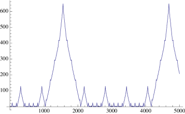
Figure 5. The $5$-adic valuation of $T(n)$

The goal of this paper is to provide a complete description of the function $\nu_{p}(T(n))$ for the primes $p=2$ and $p=3$. The case $p\geq 5$ presents similar features and the techniques described here might be used to explain the graphs shown in Figure 5 and 6. A detailed study of the graph of $\nu_{2}\circ T$ yields a new proof of a result of D. Frey and J. Sellers: the number $T(n)$ is odd if and only if $n$ is a Jacobstahl number $J_{m}$. These numbers are defined by the recurrence $J_{n}=J_{n-1}+2J_{n-2}$ with initial conditions $J_{1}=1$ and $J_{2}=3$. The proof presented here is based on the fact that the graph of $\nu_{2}(T(j))$ is formed by blocks over the intervals $\{\,[J_{n},\,J_{n+1}]:\,n\in\mathbb{N}\}$. Moreover, the part over $[J_{n+1},\,J_{n}]$ contains, at the center, a vertical shift of the graph over $[J_{n-1},\,J_{n}]$. This proves that the valuation $\nu\circ T$ can only vanish at the endpoints $J_{n}$.

Introduce a generalization of $T(n)$ as

(1.7) $$T_{p}(n):=\prod_{j=0}^{n-1}\frac{(pj+1)!}{(n+j)!}.$$

We will establish that, for each $p$, the numbers $T_{p}(n)$ are integers and examine some of their divisibility properties. A combinatorial interpretation of $T_{p}(n)$ is left as an open question.

2. A recurrence

The integers $T(n)$ grow rapidly and a direct calculation using (1.1) is impractical. The number of digits of $T(10^{k})$ is $12,\,1136,\,113622$ and $11362189$ for $1\leq k\leq 4$. Naturally, the prime factorization of $T(n)$ is more promising, since every prime $p$ dividing $T(n)$ satisfies $p\leq 3n-2$.

In this section we discuss a recurrence for the $p$-adic valuation of $T(n)$, that permits a fast computation of this function. The statement involves the function

(2.1) $$f_{p}(j):=\nu_{p}(j!).$$

Theorem 2.1.

Let $p$ be a prime. Then the $p$-adic valuation of $T(n)$ satisfies

(2.2) $$\nu_{p}(T(n+1))=\nu_{p}(T(n))+f_{p}(3n+1)+f_{p}(n)-f_{p}(2n)-f_{p}(2n+1).$$

Proof.

This follows directly from comparing the expression

(2.3) $$\nu_{p}(T(n))=\sum_{j=0}^{n-1}f_{p}(3j+1)-\sum_{j=0}^{n-1}f_{p}(n+j)$$

with the corresponding one for $\nu_{p}(T(n+1))$ and the initial value $T(1)=1$. ∎

Legendre [10] established the formula

(2.4) $$f_{p}(j)=\nu_{p}(j!)=\frac{j-S_{p}(j)}{p-1},$$

where $S_{p}(j)$ denotes the sum of the base-$p$ digits of $j$. The result of Theorem 2.1 is now expressed in terms of the function $S_{p}$.

Corollary 2.2.

The $p$-adic valuation of $T(n)$ is given by

(2.5) $$\nu_{p}(T(n))=\frac{1}{p-1}\left(\sum_{j=0}^{n-1}S_{p}(n+j)-\sum_{j=0}^{n-1}S_{p}(3j+1)\right).$$

Summing the recurrence (2.2) and using $T(1)=1$ we obtain an alternative expression for the $p$-adic valuation of $T(n)$.

Proposition 2.3.

The $p$-adic valuation of $T(n)$ is given by

(2.6) $$\nu_{p}(T(n))=\frac{1}{p-1}\sum_{j=1}^{n-1}\left(S_{p}(2j)+S_{p}(2j+1)-S_{p}(3j+1)-S_{p}(j)\right).$$

In particular, for $p=2$ we have

$$\nu_{2}(T(n)) = \sum_{j=0}^{n-1}\left(S_{2}(2j+1)-S_{2}(3j+1)\right)$$

$$= \sum_{j=1}^{n}\left(S_{2}(2j-1)-S_{2}(3j-2)\right).$$

Corollary 2.4.

For each $n\in\mathbb{N}$ we have

(2.8) $$\sum_{j=1}^{n-1}S_{2}(2j+1)\geq\sum_{j=1}^{n-1}S_{2}(3j+1).$$

Note. The formula (2.6) can be used to compute $T(n)$ for large values of $n$. Recall that only primes $p\leq 3n-2$ appear in the factorization of $T(n)$. For example, the number $T(100)$ has $1136$ digits and its prime factorization is given by

(2.9) $$T(100)=2^{23}\cdot 3^{19}\cdot 13^{13}\cdot 17^{4}\cdot 29^{3}\cdot 41^{4}\cdot 61^{2}\cdot 67^{11}\cdot 71^{5}\cdot 73^{3}\cdot 151\cdot 157^{5}\cdot 163^{9}\cdot 167^{11}\\ \times 173^{15}\cdot 179^{19}\cdot 181^{21}\cdot 191^{27}\cdot 193^{29}\cdot 197^{31}\cdot 199^{33}\cdot 211^{30}\cdot 223^{26}\cdot 227^{24}\cdot 229^{24}\cdot 233^{22}\\ \times 239^{20}\cdot 241^{40}\cdot 251^{16}\cdot 257^{14}\cdot 263^{12}\cdot 269^{10}\cdot 271^{10}\cdot 277^{8}\cdot 281^{6}\cdot 283^{6}\cdot 293^{2}.$$

The recurrence (2.2) could be employed to generate large amount of data related to number theoretical questions associated to $T(n)$. In this paper we address the simplest of all: characterize those indices $n$ for which $T(n)$ is odd.

3. When is $T(n)$ odd?

Figure 1 shows the $2$-adic valuation of the sequence $T(n)$ for $1\leq n\leq 10^{5}$. Observe that $\nu_{2}(T(n))\geq 0$ in view of the fact that $T(n)\in\mathbb{N}$. Moreover, we see that $\nu_{2}(T(n))=0$ for a sequence of values starting with

(3.1) $$1,\,3,\,5,\,11,\,21,\,43,\,85,\,171,\,341,\,683.$$

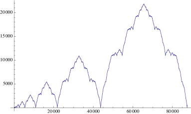
Figure 1. The $2$-adic valuation of $T(n)$

A search in The On-Line Encyclopedia of Integer Sequences identifies these numbers as terms in the Jacobsthal sequence (A001045), defined by the recurrence

(3.2) $$J_{n}=J_{n-1}+2J_{n-2},\text{ with }J_{0}=1,J_{1}=1.$$

The empirical observation is that the sequence $T(n)$ is odd if and only if $n$ is a Jacobsthal number; i.e., $n=J_{m}$ for some $m$.

Note. The Jacobsthal numbers have many interpretations. Here is a small sample:

a) $J_{n}$ is the numerator of the reduced fraction in the alternating sum

$$\sum_{j=1}^{n+1}\frac{(-1)^{j+1}}{2^{j}}.$$

b) Number of permutations with no fixed points avoiding $231$ and $132$.

c) The number of odd coefficients in the expansion of $(1+x+x^{2})^{2^{n-1}-1}$.

Many other examples can be found at

http://www.research.att.com/~njas/sequences/A001045

In this section we present a new proof of the following result [7].

Theorem 3.1.

The number $T(n)$ is odd if and only if $n$ is a Jacobstahl number.

The proof will employ several elementary properties of the Jacobsthal number $J_{n}$, summarized here for the convenience of the reader.

(3.3) $$J_{n}=J_{n-1}+2J_{n-2},\text{ with }J_{0}=1,\,J_{1}=1.$$

Lemma 3.2.

For $n\geq 2$, the Jacobstahl numbers $J_{n}$ satisfy

a) $J_{n}=J_{n-1}+2J_{n-2}$ with $J_{0}=1$ and $J_{1}=1$. (This is the definition of $J_{n}$).

b) $J_{n}=\frac{1}{3}(2^{n+1}+(-1)^{n})$.

c) $2^{n-1}+1\leq J_{n}<2^{n}$.

d) $J_{n}+J_{n-1}=2^{n}$.

e) $J_{n}-J_{n-2}=2^{n-1}$.

Outline of the proof of Theorem 3.1. The argument is based on some observations from the graph of the function $\nu_{2}\circ T$ as seen in Figure 1. The proof is divided into a small number of steps, each one verified by an inductive procedure. The hypothesis assumes complete knowledge of the function $\nu_{2}(T(j))$ for $0\leq j\leq J_{n}$. We now show how to describe the function $\nu_{2}\circ T$ in the interval $[J_{n},\,J_{n+1}].$

Step 1. The midpoint of the interval is $j=2^{n}$. The value there is $\nu_{2}(T(2^{n}))=J_{n-1}$. This is Theorem 3.4.

Step 2. The value $T(J_{n})$ is odd, that is, $\nu_{2}(T(J_{n}))=0.$ This is the content of Theorem 3.5.

Step 3. Let $0\leq i\leq 2J_{n-3}$. Then

(3.4) $$\nu_{2}(T(J_{n}+i))=i+\nu_{2}(T(J_{n-2}+i)).$$

This is Lemma 3.6. It describes the function $\nu_{2}\circ T$ in the interval $[J_{n},\,2^{n}-J_{n-2}]$. In particular, $\nu_{2}(T(2^{n}-J_{n-2}))=2J_{n-3}$ and $\nu_{2}(T(j))>0$ for $J_{n}<j<2^{n}-J_{n-2}$.

Step 4. Let $0\leq i\leq 2J_{n-2}$. Then

(3.5) $$\nu_{2}(T(2^{n}-J_{n-2}+i))=\nu_{2}(T(J_{n-1}+i))+2J_{n-3}.$$

This is Proposition 3.7. It shows that the graph of $\nu_{2}\circ T$ on the interval $[2^{n}-J_{n-2},2^{n}+J_{n-2}]$ is a vertical shift, by $2J_{n-3}$, of the graph over the interval $[J_{n-1},J_{n}]$.

Step 5. This is Proposition 3.8. Let $0\leq i\leq J_{n-1}$. Then $\nu_{2}(T(2^{n}-i))=\nu_{2}(T(2^{n}+i))$, explaining the symmetry of the graph about the point $j=2^{n}$ on the interval $[J_{n},J_{n+1}]$.

This completes the proof of Theorem 3.1.

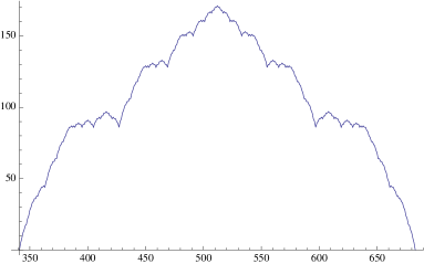
Figure 2. The $2$-adic valuation of $T(n)$ between minima

Note. As we vary $m\in\mathbb{N}$, the graph of $\nu_{2}(T(n))$ in the interval $[J_{m},J_{m+1}]$ resemble each other. These are depicted in Figure 2 that shows the value of $\nu_{2}(T(n))$ for $J_{10}=341\leq n\leq 683=J_{11}$. This suggests a possible scaling law for the graph of $\nu_{2}\circ T$. Figure 3 shows the first $15$ such graphs, scaled to the unit square. The convergence to a limiting curve is apparent. The properties of this curve will be explored in the future.

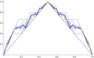
Figure 3. The scaled version of the $2$-adic valuation of $T(n)$

The proof of Theorem 3.1 begins with an auxiliary lemma.

Lemma 3.3.

Let $n\in\mathbb{N}$. Introduce the notation $S_{n,j}^{+}:=S_{2}(3\cdot 2^{n}+3j-2)$ and $S_{n,j}^{-}:=S_{2}(3\cdot 2^{n}-3j+1)$. Then

(3.6) $$S_{n,j}^{+}=\begin{cases}S_{2}(3j-2)+2&\text{ if }\quad 1\leq j\leq J_{n-1},\\ S_{2}(3j-2)&\text{ if }\quad 1+J_{n-1}\leq j\leq J_{n},\\ S_{2}(3j-2)+1&\text{ if }\quad 1+J_{n}\leq j\leq 2^{n};\end{cases}$$

and

(3.7) $$S_{n,j}^{-}=\begin{cases}n+1-S_{2}(3j-2)&\text{ if }\quad 1\leq j\leq J_{n-1},\\ n+2-S_{2}(3j-2)&\text{ if }\quad 1+J_{n-1}\leq j\leq J_{n},\\ n+1-S_{2}(3j-2)&\text{ if }\quad 1+J_{n}\leq j\leq 2^{n}.\end{cases}$$

Proof.

Let $3j-2=a_{0}+2a_{1}+\cdots+a_{r}2^{r}$ be the binary expansion of $3j-2$. The corresponding one for $3\cdot 2^{n-1}$ is simply $2^{n-1}+2^{n}$. For $3j-2<2^{n-1}$ these two expansions have no terms in common, therefore $S_{n,j}^{+}=S_{2}(3j-2)+2$. On the other hand, if $2^{n-1}\leq 3j-2<2^{n}$ then the index in the binary expansion of $3j-2$ is $r=n-1$ with $a_{n-1}=1$. The expansion of $3j-2+3\cdot 2^{n-1}$ is now

$$a_{0}+2a_{1}+\cdots+a_{n-2}2^{n-2}+2^{n-1}+2^{n-1}+2^{n}=a_{0}+2a_{1}+\cdots+a_{n-2}2^{n-2}+2^{n+1},$$

and this yields $S_{n,j}^{+}=a_{0}+a_{1}+\cdots+a_{n-2}+1=S_{2}(3j-2)$. The remaining cases are treated in a similar form. ∎

We now establish the $2$-adic valuation at the center of the interval $[J_{n-1},J_{n}]$. This completes Step 1 in the outline.

Theorem 3.4.

Let $n\in\mathbb{N}$. Then

(3.8) $$\nu_{2}\left(T\left(2^{n}\right)\right)=J_{n-1}.$$

Proof.

We proceed by induction and split

(3.9) $$\nu_{2}\left(T(2^{n})\right)=\sum_{j=1}^{2^{n}-1}\left[S_{2}(2j+1)-S_{2}(3j+1)\right]$$

at $j=2^{n-1}-1$. The first part is identified as $\nu_{2}\left(T(2^{n-1})\right)$ to produce

$$\nu_{2}\left(T(2^{n})\right)=\nu_{2}\left(T(2^{n-1})\right)+\sum_{j=0}^{2^{n-1}-1}S_{2}(2j+1+2^{n})-\sum_{j=1}^{2^{n-1}}S_{2}(3j-2+3\cdot 2^{n-1}).$$

Now observe that $2j+1\leq 2^{n}-1<2^{n}$ so that $S_{2}(2j+1+2^{n})=S_{2}(2j+1)+1$. Lemma 3.3 gives, for $n$ even,

(3.10) $$\sum_{j=1}^{2^{n-1}}S_{2}(3j-2+3\cdot 2^{n-1})=\sum_{j=1}^{(2^{n-1}+1)/3}[S_{2}(3j-2)+2]+\\ \sum_{j=(2^{n-1}+1)/3}^{(2^{n}-1)/3}S_{2}(3j-2)+\sum_{j=(2^{n}+2)/3}^{2^{n-1}}[S_{2}(3j-2)+1]$$

and using (2.3) yields

(3.11) $$\nu_{2}(T(2^{n}))=2\nu_{2}(T(2^{n-1}))-1=2J_{n-2}-1.$$

Elementary properties of Jacobsthal numbers show that $2J_{n-2}-1=J_{n-1}$ proving the result for $n$ even. The argument for $n$ odd is similar. ∎

The next theorem corresponds to Step 2 of the outline.

Theorem 3.5.

Let $n\in\mathbb{N}$. Then $T(J_{n})$ is odd.

Proof.

Proposition 2.3 gives

(3.12) $$\nu_{2}\left(T(J_{n})\right)=\sum_{j=1}^{J_{n}-1}\left[S_{2}(2j+1)-S_{2}(3j+1)\right].$$

Observe that $2^{n-1}\leq J_{n}-1$, so

$$\nu_{2}\left(T(J_{n})\right) = \sum_{j=1}^{2^{n-1}-1}\left[S_{2}(2j+1)-S_{2}(3j+1)\right]+$$

$$+\sum_{j=2^{n-1}}^{J_{n}-1}\left[S_{2}(2j+1)-S_{2}(3j+1)\right]$$

$$= \nu_{2}\left(T(2^{n-1})\right)+\sum_{j=2^{n-1}}^{J_{n}-1}\left[S_{2}(2j+1)-S_{2}(3j+1)\right].$$

Therefore

$$\nu_{2}\left(T(J_{n})\right)=\nu_{2}(T(2^{n-1}))+\sum_{j=0}^{J_{n}-1-2^{n-1}}\left[S_{2}(2j+1+2^{n})-S_{2}(3j+1+3\cdot 2^{n-1})\right].$$

The elementary properties of Jacobsthal numbers give

(3.13) $$J_{n}-1-2^{n-1}=J_{n-2}-1,$$

so that

$$\nu_{2}\left(T(J_{n})\right)=\nu_{2}(T(2^{n-1}))+\sum_{j=0}^{J_{n-2}-1}\left[S_{2}(2j+1+2^{n})-S_{2}(3j+1+3\cdot 2^{n-1})\right].$$

Observe that

$$2j+1\leq 2(J_{n-2}-1)+1=2J_{n-2}-1=J_{n}-J_{n-1}-1<2^{n},$$

resulting in

$$S_{2}(2j+1+2^{n})=S_{2}(2j+1)+1.$$

Similarly $3j+1\leq 3J_{n-2}-2<3(2^{n-1}+(-1)^{n})-2\leq 2^{n-1}-1$ and from $3\cdot 2^{n-1}=2^{n}+2^{n-1}$ we obtain

$$S_{2}(3j+1+3\cdot 2^{n-1})=S_{2}(3j+1)+2,$$

for $0\leq j\leq J_{n-2}-1$. It follows that

$$\nu_{2}\left(T(J_{n})\right)=\nu_{2}\left(T(2^{n-1})\right)+\sum_{j=0}^{J_{n-2}-1}\left[S_{2}(2j+1)-S_{2}(3j+1)\right]-J_{n-2}.$$

Theorem 3.4 shows that the first and third term on the line above cancel, leading to

$$\nu_{2}\left(T(J_{n})\right)=\nu_{2}\left(T(J_{n-2})\right).$$

The result now follows by induction on $n$. ∎

We continue with the proof of Theorem 3.1. The next Lemma corresponds to Step 3 in the outline. It describes the values $\nu_{2}(T(j))$ for $J_{n}\leq j\leq J_{n}+2J_{n-3}=2^{n}-J_{n-2}$. The result of Lemma 3.6 shows that $\nu_{2}(T(j))>0$ for $J_{n}<j<2^{n}-J_{n-2}$.

Lemma 3.6.

For $0<i\leq 2J_{n-3}$ we have

(3.14) $$\nu_{2}(T(J_{n}+i))=i+\nu_{2}(T(J_{n-2}+i)).$$

Proof.

Assume that $n$ is even and consider

$$\nu_{2}(T(J_{n}+i)) = \sum_{j=1}^{J_{n}+i-1}\left[S_{2}(2j+1)-S_{2}(3j+1)\right]$$

$$= \sum_{j=1}^{J_{n}-1}\left[S_{2}(2j+1)-S_{2}(3j+1)\right]+\sum_{j=J_{n}}^{J_{n}+i-1}\left[S_{2}(2j+1)-S_{2}(3j+1)\right].$$

The first sum is $\nu_{2}(T(J_{n}))=0$, according to Theorem 3.5. Therefore, using Lemma 3.2 we have

$$\nu_{2}(T(J_{n}+i)) = \sum_{j=J_{n}}^{J_{n}+i-1}\left[S_{2}(2j+1)-S_{2}(3j+1)\right]$$

$$= \sum_{j=J_{n}+1}^{J_{n}+i}\left[S_{2}(2j-1)-S_{2}(3j-2)\right]$$

$$= \sum_{j=J_{n}+1-2^{n-1}}^{J_{n}+i-2^{n-1}}\left[S_{2}(2^{n}+2j-1)-S_{2}(3\cdot 2^{n-1}+3j-2)\right]$$

$$= \sum_{j=J_{n-2}+1}^{J_{n-2}+i}\left[S_{2}(2^{n}+2j-1)-S_{2}(3\cdot 2^{n-1}+3j-2)\right].$$

The index $j$ satisfies

$$2j-1\leq 2(J_{n-2}+i)-1<2(J_{n-2}+2J_{n-3})=2J_{n-1}<2^{n},$$

therefore $S_{2}(2^{n}+2j-1)=1+S_{2}(2j-1)$.

The lower limit in the last sum is $J_{n-2}+1=\frac{1}{3}(2^{n-1}+1)+1$, and the upper bound is

(3.15) $$J_{n-2}+i\leq J_{n-2}+2J_{n-3}=J_{n-1}=\frac{1}{3}(2^{n}-1).$$

Lemma 3.3 gives $S_{2}(3\cdot 2^{n-1}+3j-2)=S_{2}(3j-2)$. Therefore

$$\nu_{2}(T(J_{n}+i)) = \sum_{j=J_{n-2}+1}^{J_{n-2}+i}\left[S_{2}(2j-1)+1-S_{2}(3j-2)\right]$$

$$= i+\sum_{j=J_{n-2}+1}^{J_{n-2}+i}\left[S_{2}(2j-1)-S_{2}(3j-2)\right]$$

$$= i+\nu_{2}(T(J_{n-2}+i)).$$

The result has been established for $n$ even. The proof for $n$ odd is similar. ∎

The next result shows the graph of $\nu_{2}\circ T$ on the interval $[2^{n}-J_{n-2},2^{n}+J_{n-2}]$ is a vertical shift of the graph on $[J_{n-1},J_{n}]$. This corresponds to Step 4 in the outline.

Proposition 3.7.

For $0\leq i\leq 2J_{n-2}$,

(3.16) $$\nu_{2}(T(2^{n}-J_{n-2}+i))=\nu_{2}(T(J_{n-1}+i))+\omega_{n},$$

where $\omega_{n}=2J_{n-3}$ is independent of $i$.

Proof.

We prove that the graph of $\nu_{2}(T(J_{n-1}+i))$ and $\nu_{2}(T(2^{n}-J_{n-2}+i))$ have the same discrete derivative. This amounts to checking the identity

(3.17) $$\nu_{2}(T(J_{n-1}+i))-\nu_{2}(T(J_{n-1}+i-1))=\\ \nu_{2}(T(2^{n}-J_{n-2}+i))-\nu_{2}(T(2^{n}-J_{n-2}+i-1))$$

for $1\leq i\leq 2J_{n-2}$. Observe that

(3.18) $$\nu_{2}(T(k))-\nu_{2}(T(k-1))=S_{2}(2k-1)-S_{2}(3k-2),$$

and using $2^{n}-J_{n-2}=2^{n-1}+J_{n-1}$, we conclude that the result is equivalent to the identity

(3.19) $$S_{2}(2^{n}+2(J_{n-1}+i)-1)-S_{2}(2(J_{n-1}+i)-1)=\\ S_{2}(3\cdot 2^{n-1}+3(J_{n-1}+i)-2)-S_{2}(3(J_{n-1}+i)-2),$$

for $1\leq i\leq 2J_{n-2}$. Define

(3.20) $$h_{n}(i)=\begin{cases}1\quad&\text{ if }1\leq i\leq J_{n-2};\\ 0\quad&\text{ if }J_{n-2}+1\leq i\leq 2J_{n-2}.\end{cases}$$

The assertion is that both sides in (3.19) agree with $h_{n}(i)$. The analysis of the left hand side is easy: the condition $1\leq i\leq J_{n-2}$ implies $2(J_{n-1}+i)-1\leq 2^{n}-1$. Thus, the term $2^{n}$ does not interact with the binary expansion $2(J_{n-1}+i)-1$ and produces the extra $1$. On the other hand, if $J_{n-2}+1\leq i\leq 2J_{n-2}$, then

(3.21) $$2^{n}+1=2(J_{n-1}+J_{n-2}+1)-1\leq 2(J_{n-1}+i)-1\\ \leq 2(J_{n-1}+2J_{n-2})-1=2J_{n}-1<2^{n+1}-1.$$

We conclude that the binary expansion of $x:=2(J_{n-1}+i)-1$ is of the form $a_{0}+a_{1}\cdot 2+\cdots+a_{n-1}\cdot 2^{n-1}+1\cdot 2^{n}$. It follows that $2^{n}+x$ and $x$ have the same number of $1$’s in their binary expansion. Thus $S_{2}(x)=S_{2}(x+2^{n})$ as claimed.

The analysis of the right hand side of (3.19) is slightly more difficult. Let $x:=3(J_{n-1}+i)-2$ and it is required to compare $S_{2}(x)$ and $S_{2}(3\cdot 2^{n-1}+x)$. Observe that

(3.22) $$x\leq 3(J_{n-1}+2J_{n-2})-2=3J_{n}-2=2^{n+1}+(-1)^{n}-2<2^{n+1}$$

and

(3.23) $$x\geq 3(J_{n-1}+1)-2=2^{n}+(-1)^{n-1}+1\geq 2^{n}.$$

We conclude that the binary expansion of $x$ is of the form

(3.24) $$x=a_{0}+a_{1}\cdot 2+\cdot+a_{n-1}\cdot 2^{n-1}+1\cdot 2^{n},$$

and the corresponding one for $3\cdot 2^{n-1}$ is $2^{n}+2^{n-1}$. An elementary calculation shows that $S_{2}(x+3\cdot 2^{n-1})-S_{2}(x)$ is $1$ if $a_{n-1}=0$ and $0$ if $a_{n-1}=1$. In order to transform this inequality to a restriction on the index $i$, observe that $a_{n-1}=1$ is equivalent to $x-2^{n}\geq 2^{n-1}$. Using the value of $x$ this becomes $3(J_{n-1}+i)-2)\geq 3\cdot 2^{n-1}$. This is directly transformed to $i\geq J_{n-2}+1$. This shows that the right hand side of (3.19) also agrees with $h_{n}$ and (3.19) has been established. ∎

The final step in the proof of Theorem 3.1, outlined as Step 5, shows the symmetry of the graph of $\nu_{2}(T(j))$ about the point $j=2^{n}$. The range covered in the next proposition is $2^{n}-J_{n-1}\leq j\leq 2^{n}+J_{n-1}$.

Proposition 3.8.

For $1\leq i\leq J_{n-1}$,

(3.25) $$\nu_{2}(T(2^{n}-i))=\nu_{2}(T(2^{n}+i)).$$

Proof.

Start with

$$\nu_{2}(T(2^{n}))-\nu_{2}(T(2^{n}-i)) = \sum_{j=2^{n}-i+1}^{2^{n}}\left[S_{2}(2j-1)-S_{2}(3j-2)\right]$$

$$= \sum_{k=1}^{i}\left[S_{2}(2^{n+1}-(2k-1))-S_{2}(3\cdot 2^{n}-(3k-1))\right].$$

The first term in the sum satisfies

(3.26) $$S_{2}(2^{n+1}-(2k-1))=n+2-S_{2}(2k-1).$$

To check this, write $2k-1=a_{0}+a_{1}\cdot 2+\cdots+a_{r}\cdot 2^{r}$ with $a_{0}=1$ because $2k-1$ is odd. Now, $2^{n+1}=(1+2+2^{2}+\cdots+2^{n})+1$ and we conclude that

$$2^{n+1}-(2k-1) = (2^{n}+2^{n-1}+\cdots+2^{r+1})$$

$$+(1-a_{r})\cdot 2^{r}+(1-a_{r+1})\cdot 2^{r-1}+\cdots+(1-a_{1})\cdot 2+1$$

Therefore

$$S_{2}(2^{n+1}-(2k-1)) = n+1-\left(a_{r}+a_{r-1}+\cdots+a_{1}\right)$$

$$= n+2-S_{2}(2k-1).$$

We conclude that

(3.27) $$\nu_{2}(T(2^{n}))-\nu_{2}(T(2^{n}-i))=(n+2)i-\sum_{k=1}^{i}S_{2}(2k-1)-\\ \sum_{k=1}^{i}S_{2}(3\cdot 2^{n}-(3k-1)).$$

Similarly

$$\nu_{2}(T(2^{n}+i))-\nu_{2}(T(2^{n})) = \sum_{j=2^{n}+1}^{2^{n}+i}\left(S_{2}(2j-1)-S_{2}(3j-2)\right)$$

$$= \sum_{k=1}^{i}\left(S_{2}(2^{n+1}+2k-1)-S_{2}(3\cdot 2^{n}+3k-2)\right).$$

The inequality

(3.28) $$2k-1\leq 2i-1\leq 2J_{n-1}-1\leq 2\cdot 2^{n-1}-1\leq 2^{n}-1<2^{n+1}$$

shows that $S_{2}(2^{n+1}+2k-1)=1+S_{2}(2k-1)$. Lemma 3.3 yields the identity

(3.29) $$S_{2}(3\cdot 2^{n}+3k-2)+S_{2}(3\cdot 2^{n}-3k+1)=n+3.$$

Therefore

$$\nu_{2}(T(2^{n}+i))-\nu_{2}(T(2^{n})) = \sum_{k=1}^{i}\left(S_{2}(2^{n+1}+2k-1)-S_{2}(3\cdot 2^{n}+3k-2)\right)+i$$

$$+\sum_{k=1}^{i}S_{2}(2k-1)-\left(n+3-S_{2}(3\cdot 2^{n}-3k+1)\right).$$

It follows that

$$\nu_{2}(T(2^{n}))-\nu_{2}(T(2^{n}-i))=-\left[\nu_{2}(T(2^{n}-i))-\nu_{2}(T(2^{n}))\right],$$

and symmetry has been established. ∎

Note. The identity (3.29) can be given a direct proof by inducting on $k$. It is required to check that the left hand side is independent of $k$ and this follows from the identity

(3.30) $$S_{2}(m+3)-S_{2}(m)=\begin{cases}2-\omega_{2}\left(\frac{m}{2}\right)\quad\text{ if }m\equiv 0\bmod 2;\\ -\omega_{2}\left(\lfloor{{{m}\over{4}}\rfloor}\right)\quad\text{ if }m\equiv 1\bmod 2.\end{cases}$$

Here $\omega_{2}(m)$ is the number of trailing $1$’s in the binary expansion of $m$. For $m=829$ we have $S_{3}(829)=7$ and $S_{3}(832)=3$. The binary expansion of $m=207=\lfloor{829/4\rfloor}$ is $11001111$ and the number of trailing $1^{\prime}s$ is $4$. This observation is due to A. Straub.

The next result shows that every positive integer $k$ is attained as $\nu_{2}(T(n))$.

Theorem 3.9.

Every nonnegative integer appears as $\nu_{2}(T(n))$ for some $n$, i.e.,

$$\mathbb{N}=\{\nu_{2}(T(n))\,:n\in\mathbb{N}\}.$$

Furthermore, each positive integer $m$ appears only finitely many times, and the last appearance is when $n=J_{2m+1}-1$.

Proof.

From the results before, we know that

$$\nu_{2}(T(J_{n}+i))>\nu_{2}(T(J_{n}+1))=\nu_{2}(T(J_{n+1}-1)),$$

for $1<i<J_{n+1}-J_{n}-2$ and $\nu_{2}(T(J_{n+2}-1))=\nu_{2}(T(J_{n}-1))+1$. This shows that the minimum values of the graph of $\nu_{2}(T(n))$ around $2^{n}$ are attained exactly at $J_{n}+1$ and $J_{n+1}-1$. These values are also strictly increasing along the even and odd indices. Thus, $m<\nu_{2}(T(i))$ for any given $m$, provided $i$ is large enough.

To determine the last appearance of $m$, we only need to determine the last occurance of $n$ such that $\nu_{2}(T(J_{n}-1))=m$. Since $\nu_{2}(T(J_{2}-1))=\nu_{2}(T(J_{3}-1))=1,$ we conclude that $\nu_{2}(T(J_{2n}-1))=\nu_{2}(T(J_{2{n+1}}-1))=n$. Therefore the last occurance for $m$ is at $J_{2m+1}-1$. ∎

Note. Define $\lambda(m)$ to be the number $m$ is attained by $\nu\circ T$. The values for $1\leq m\leq 8$ are shown below.

$m$	1	2	3	4	5	6	7	8
$\lambda(m)$	2	8	5	12	5	14	8	14

Table 1. The first $8$ values in the range of $\nu_{2}\circ T$

For example, the values of $n$ for which $\nu(T(n))=5$ are $16,\,342,\,682,\,684$ and $J_{11}-1=1364$ and the eight solutions to $\nu(T(n))=7$ are $26,\,38,\,46,\,82,\,5462,\newline \,10922,\,10924$ and $J_{15}-1=21844$.

Note. In sharp contrast to the $2$-adic valuation, D. Frey and J. Sellers [8, 9] show that if $p\geq 3$ is a prime, then for each nonnegative integer $m$ there exist infinitely many positive integers $n$ for which $\nu_{p}(T(n))=m$.

4. The $3$-adic valuation of $T(n)$

The analysis of the $2$-adic valuation of $T(n)$ is now extended to the prime $p=3$. The discussion employs the expansion of $n\in\mathbb{N}$ in base $3$, given by

(4.1) $$n=a_{0}+a_{1}\cdot 3+a_{2}\cdot 3^{2}+\cdots+a_{r}\cdot 3^{r}$$

and the function

(4.2) $$S_{3}(n):=a_{0}+a_{1}+\cdots+a_{r}.$$

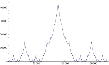
Figure 4. The $3$-adic valuation of $T(n)$

Figure 4 presents a well-defined symmetry for $\nu_{3}(T(n))$. This is explained in Theorem 4.4.

The first result characterizes the values $n$ for which $\nu_{3}(T(n))=0$.

Theorem 4.1.

Let $n\in\mathbb{N}$ with (4.1) as its expansion in base $3$. Then $\nu_{3}(T(n))=0$ if and only if there is an index $0\leq i\leq r$ such that $a_{0}=a_{1}=\cdots=a_{i-1}=0$ and $a_{i+1}=a_{i+2}=\cdots=a_{r}=0\text{ or }2$, with $a_{i}$ arbitrary.

We begin with some elementary results on the function $S_{3}$ which admit elementary proofs.

Lemma 4.2.

Let $n\in\mathbb{N}$. Then

$$S_{3}(3n)=S_{3}(n),\,S_{3}(3n+1)=1+S_{3}(n)\text{ and }S_{3}(3n+2)=2+S_{3}(n).$$

Lemma 4.3.

Let $n\in\mathbb{N}$. Then

$$S_{3}(4\cdot 3^{n}+b) = 2+S_{3}(b)\text{ for all }0\leq b<2\cdot 3^{n},$$

$$S_{3}(2\cdot 3^{n}+b) = 2+S_{3}(b)\text{ for all }0\leq b<3^{n},$$

$$S_{3}(3^{n}+b-1) = 1+S_{3}(b-1)\text{ for }1\leq b<3^{n}.$$

The next step in analyzing the function $\nu_{3}\circ T$ is to produce a recurrence for this valuation. The symmetry observed in Figure 4 is a consequence of this result.

Proposition 4.4.

Let $n\in\mathbb{N}$. Then $\nu_{3}(T(3n))=3\nu_{3}(T(n))$.

Proof.

Legendre’s formula (2.2) shows that the result is equivalent to

(4.3) $$\sum_{j=0}^{3n-1}S_{3}(3n+j)-\sum_{j=0}^{3n-1}S_{3}(3j+1)-3\sum_{j=0}^{n-1}S_{3}(n+j)+3\sum_{j=0}^{n-1}S_{3}(3j+1)=0.$$

Each term of (4.3) is now simplified. Lemma 4.2 shows that

$$\sum_{j=0}^{3n-1}S_{3}(3n+j) = \sum_{j=0}^{n-1}S_{3}(3(n+j))+\sum_{j=0}^{n-1}S_{3}(3(n+j)+1)+\sum_{j=0}^{n-1}S_{3}(3(n+j)+2)$$

$$= 3n+3\sum_{j=0}^{n-1}S_{3}(n+j),$$

and

$$\sum_{j=0}^{3n-1}S_{3}(3j+1) = 3n+\sum_{j=0}^{3n-1}S_{3}(j)$$

$$= 3n+\sum_{j=0}^{n-1}S_{3}(3j)+\sum_{j=0}^{n-1}S_{3}(3j+1)+\sum_{j=0}^{n-1}S_{3}(3j+2)$$

$$= 6n+3\sum_{j=0}^{n-1}S_{3}(j),$$

and, finally,

$$\sum_{j=0}^{n-1}S_{3}(3j+1) = n+\sum_{j=0}^{n-1}S_{3}(j).$$

These identities show that the left-hand side of (4.3) vanishes. ∎

Corollary 4.5.

For each $n\in\mathbb{N}$, we have $\nu_{3}(T(3^{n}))=\nu_{3}(T(2\cdot 3^{n}))=0.$

Proof.

This follows directly from $T(1)=1$ and $T(2)=1$ and Proposition 4.4. ∎

For brevity, introduce the function

(4.4) $$\mu_{3}({j}):=S_{3}(2j)+S_{3}(2j+1)-S_{3}(3j+1)-S_{3}(j).$$

Thus Proposition 2.3 takes the form

(4.5) $$\nu_{3}(T(n))=\tfrac{1}{2}\sum_{j=1}^{n-1}\mu_{3}({j}).$$

Observe that

(4.6) $$\mu_{3}({n-1})=2\left(\nu_{3}(T(n))-\nu_{3}(T(n-1))\right).$$

Proposition 4.6.

If $0\leq a\leq 3^{n}$ then $\nu_{3}(T(a))=\nu_{3}(T(2\cdot 3^{n}+a))$.

Proof.

The limiting cases $a=0$ and $a=3^{n}$ follow from Corollary 4.5. The result follows from (4.5) and the identities $\mu_{3}({a})=\mu_{3}({2\cdot 3^{n}+a})$ for $1\leq a\leq 3^{n},$ that are direct consequence of Lemma 4.3. ∎

The proof of Theorem 4.1 is presented next.

Proof.

Consider the representation of $n\in\mathbb{N}$ in base $3$:

(4.7) $$n=a_{0}+3a_{1}+3^{2}a_{2}+\cdots+3^{r}a_{r}.$$

Corollary 4.5 and Proposition 4.6 show that the numbers $n$ with the form stated in the theorem satisfy $\nu_{3}(T(n))=0$. We need to prove that these are the only zeros of $\nu_{3}\circ T$.

The proof is by induction and show that $\nu_{3}(T(a))>0$ for $3^{n}<a<3^{n+1}$. Proposition 4.6 shows that, if $a_{r}=2$, then $\nu_{3}(T(n))>0$. Proposition 4.7 treats the result for $a_{r}=1$ and the first half of these numbers $0\leq a-3^{r}\leq 3^{r}$. Proposition 4.9 establishes a symmetry result that takes care of the second half.
∎

We now establish the symmetry of the function $\nu_{3}\circ T$. The proof begin with some auxiliary steps.

Proposition 4.7.

Let $n,\,a\in\mathbb{N}$ and assume $1\leq a<3^{n}$. Then

$$\mu_{3}({3^{n}+a})=\left\{\begin{array}[]{lll}\mu_{3}({a})+2&\text{if }1\leq a<\tfrac{1}{2}3^{n};\\ \mu_{3}({a})&\text{if }a=\tfrac{1}{2}(3^{n}+1);\\ \mu_{3}({a})-2&\text{if }\tfrac{1}{2}3^{n}+1<a\leq 3^{n}.\end{array}\right.$$

Proof.

When $1\leq b<\tfrac{1}{2}3^{n}$, the first part follows from Lemma 4.3. The other parts can be proved similarly, and thus omitted. ∎

Lemma 4.8.

If $3\nmid a$, $3\nmid b$, $n<m$, and $b<3^{m-n}$, then

(4.8) $$\nu_{3}(T(3^{m}a-3^{n}b))=2(m-n)+\nu_{3}(T(a))-\nu_{3}(T(b)).$$

Proposition 4.9.

If $1\leq i<\frac{3^{n}}{2}$, $\mu_{3}({3^{n}+i})=-\mu_{3}({2\cdot 3^{n}-i+1})$.

Proof.

Let $A=3^{n}+i$ and $B=2\cdot 3^{n}-i+1$. We prove $\mu_{3}({A})=-\mu_{3}({B})$.

First we observe that

$$\mu_{3}({A}) = S_{3}(2\cdot 3^{n}+2i-1)+S_{3}(2\cdot 3^{n}+2i-2)-S_{3}(3^{n+1}+2i-2)-S_{3}(3^{n}+i-1)$$

$$= (2+S_{3}(2i-1))+(2+S_{3}(2i-2))-(1+S_{3}(3i-2))-(1+S_{3}(i-1)$$

$$= S_{3}(2i-1)+S_{3}(2i-2)-S_{3}(3i-2)-S_{3}(i-1)+2.$$

There are three cases to consider according to the value of $i$ modulo $3$. Assume first that $i\equiv 0\bmod 3$ and write $i=3^{a}x$, where $a>0$ and $3\nmid x$. Then

$$\mu_{3}({A}) = S_{3}(2i-1)+S_{3}(2i-2)-S_{3}(3i-2)-S_{3}(i-1)+2$$

$$= S_{3}(2\cdot 3^{a}x-1)+S_{3}(2\cdot 3^{a}x-2)-S_{3}(3\cdot 3^{a}x-2)-S_{3}(3^{a}x-1)+2$$

$$= (S_{3}(2x)-1+2a)+(S_{3}(2x)-2+2a)-$$

$$(S_{3}(x)-2+2(a+1))-(S_{3}(x)-1+2a)+2$$

$$= 2S_{3}(2x)-2S_{3}(x)$$

$$\mu_{3}({B}) = S_{3}(4\cdot 3^{n}-2i+1)+S_{3}(4\cdot 3^{n}-2i)-S_{3}(2\cdot 3^{n+1}-3i+1)-S_{3}(2\cdot 3^{n}-i)$$

$$= S_{3}(4\cdot 3^{n}-2\cdot 3^{a}x+1)+S_{3}(4\cdot 3^{n}-2\cdot 3^{a}x)$$

$$-S_{3}(2\cdot 3^{n+1}-2\cdot 3^{a+1}x+1)-S_{3}(2\cdot 3^{n}-3^{a}x)$$

$$= (2n+2-S_{3}(2\cdot 3^{a}x-1))+(2(n-a)+2-S_{3}(2x))$$

$$-(2n+4-S_{3}(2\cdot 3^{a+1}x+1))-(2(n-a)+2-S_{3}(x))$$

$$= (-S_{3}(2x)+1)+(-S_{3}(2x))-(-S_{3}(2x)-1)-(-S_{3}(x))-2$$

$$= -2S_{3}(2x)+2S_{3}(x)=-\mu_{3}({A}),$$

as claimed. The cases $i\equiv 1,\,2\bmod 3$ are analyzed by similar techniques. ∎

Note. The techniques outlined in this paper can be used to present a complete description of the function $\nu_{p}(T(n))$ for $p\geq 5$ prime. We limit ourselves to showing the graphs for $p=5$ and $7$ in the range $n\leq 5000$.

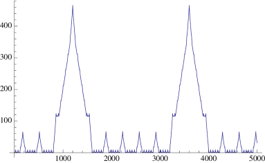
Figure 6. The $7$-adic valuation of $T(n)$

The rest of the section is devoted to develop an efficient procedure to compute $\nu_{3}(T(n))$. We begin with the ternary expansion of $n$

(4.9) $$n=\sum_{i=0}^{k}a_{i}3^{i},$$

and now define two sequence of integers:

(4.10) $$n_{k}=n_{k}^{\prime}=n,$$

and, for $0\leq j<k$ and assume having

(4.11) $$n^{\prime}_{j+1}=\sum^{j+1}_{i=0}b_{j+1,i}3^{i},$$

then define recursively

$$n_{j} = \sum^{j}_{i=0}b_{j+1,i}3^{i},$$

$$n^{\prime}_{j} = \left\{\begin{array}[]{lll}n_{j}&\text{if }b_{j+1,j+1}=0,2;\\ \min(n_{j},3^{j+1}-n_{j})&\text{if }b_{j+1,j+1}=1.\end{array}\right.$$

Theorem 4.10.

The $3$-adic valuation of $T(n)$ satisfies

(4.13) $$\nu_{3}(T(n_{j}))=\left\{\begin{array}[]{lll}\nu_{3}(T(n^{\prime}_{j-1}))&\text{if }a_{j}=0,2;\\ \nu_{3}(T(n^{\prime}_{j-1}))+2n^{\prime}_{j-1}&\text{if }a_{j}=1.\end{array}\right.$$

Note. Observe that the time required to calculate $\nu_{3}(T(n))$ is $O(n^{2}\ln n)$ using the definition of $T(n)$. Using Proposition 2.3 the computational time reduces to $O(n)$. The method described in Theorem 4.10 further reduces this time to $O(\ln n)$. A similar algorithm can be developed for $p=2$.

Example. Let $n=1280$, whose representation with base 3 is $1202102$. Then $k=6$ and we have

$j$	$n_{j}$	$n_{j}$ (base 3)	$n^{\prime}_{j}$	$n^{\prime}_{j}$ (base 3)
6	1280	1202102	1280	1202102
5	551	202102	178	020121
4	178	20121	178	20121
3	16	0102	16	0102
2	16	102	16	102
1	7	21	2	02
0	2	2	1	1

Table 2. The fast algorithm for $\nu_{3}\circ T$

It follows that

$$\nu_{3}(T(1280)) = 2n^{\prime}_{5}+\nu_{3}(T(n^{\prime}_{5}))$$

$$= 2n^{\prime}_{5}+\nu_{3}(T(n_{2}))$$

$$= 2n^{\prime}_{5}+2\nu_{3}(T(n^{\prime}_{1}))+\nu_{3}(T(n_{1}))$$

$$= 360.$$

5. A generalization

The sequence

(5.1) $$T_{p}(n):=\prod_{j=0}^{n-1}\frac{(pj+1)!}{(n+j)!},$$

contains $T(n)$ of (1.1) as the special case $T(n)=T_{3}(n)$. In this section we present some elementary properties of this generalization.

Theorem 5.1.

For a fixed prime $p\geq 3$, the numbers $T_{p}(n)$ are integers.

Proof.

Observe that

(5.2) $$T_{p}(n+1)=T_{p}(n)\times\frac{(pn+1)!\,n!}{(2n+1)!\,(2n)!}.$$

Define

(5.3) $$x_{p}(n):=\frac{(pn+1)!}{((p-1)n+1)!\,n!}=\binom{pn+1}{n},$$

and observe that

(5.4) $$\frac{(pn+1)!\,n!}{(2n+1)!\,(2n)!}=x_{p}(n)\times\frac{((p-1)n+1)!}{(2n+1)!\,(2n)!}n!^{2}.$$

Iterating this argument yields

(5.5) $$\frac{(pn+1)!\,n!}{(2n+1)!\,(2n)!}=\prod_{r=0}^{k-1}x_{p-r}(n)\times\frac{((p-k)n+1)!}{(2n+1)!\,(2n)!}n!^{k+1}.$$

The choice $k=p-4$ confirms that

$$\frac{(pn+1)!\,n!}{(2n+1)!\,(2n)!}=\binom{4n+1}{2n}\,n!^{p-3}\prod_{r=0}^{p-5}\binom{(p-r)n+1}{n}$$

is an integer. The recurrence (5.2) and the initial condition $T_{p}(1)=1$ now show that $T_{p}(n)$ is also an integer. The explicit formula

(5.6) $$T_{p}(n)=\prod_{j=1}^{n-1}\binom{4j+1}{2j}j!^{p-3}\prod_{r=0}^{p-5}\binom{(p-r)j+1}{j}$$

follows from the recurrence.
∎

Proof.

An alternative proof of the fact that $\displaystyle\frac{(pn+1)!n!}{(2n+1)!\,(2n)!}$ is an integer was shown to us by Valerio de Angelis. Observe that, for $p\geq 4$, we have $(pn+1)!=N\times(4n+1)!$ for the integer $N=(4n+2)_{(p-4)n}$. Therefore

(5.7) $$\frac{(pn+1)!\,n!}{(2n+1)!\,(2n)!}=(4n+2)_{(p-4)n}\times\binom{4n+2}{2n}n!.$$

This leads to the explicit formula

(5.8) $$T_{p}(n)=\prod_{j=1}^{n-1}(4j+2)_{(p-4)n}\binom{4j+1}{2j}j!.$$

∎

Proof.

A third proof using Theorem 1.1 was shown to us by T. Amdeberhan. The required inequality states: if $n,k,p\in\mathbb{N}$ and $p\geq 3$, then

$$\psi_{k}(n;p):=\sum_{j=0}^{n-1}\left\lfloor{{pj+1}\over{k}}\right\rfloor-\sum_{j=0}^{n-1}\left\lfloor{{n+j}\over{k}}\right\rfloor\geq 0.$$

It suffices to prove the special case $p=3$, i.e. $\psi_{k}(n;3)\geq 0$ which we denote by $\psi_{k}(n)$ for $k\geq 3,n\geq 1$. Write $n=ck+r$ where $0\leq r\leq k-1$. We approach a reduction process by breaking down the respective sums as follows.

$$\sum_{j=0}^{n-1}\left\lfloor{{3j+1}\over{k}}\right\rfloor = \sum_{j=0}^{ck-1}\left\lfloor{{3j+1}\over{k}}\right\rfloor+\sum_{j=0}^{r-1}\left\lfloor{{3(ck+j)+1}\over{k}}\right\rfloor$$

$$= \sum_{j=0}^{ck-1}\left\lfloor{{3j+1}\over{k}}\right\rfloor+3cr+\sum_{j=0}^{r-1}\left\lfloor{{3j+1}\over{k}}\right\rfloor,$$

and

$$\sum_{j=0}^{n-1}\left\lfloor{{n+j}\over{k}}\right\rfloor = \sum_{j=0}^{ck-1}\left\lfloor{{ck+r+j}\over{k}}\right\rfloor+2cr+\sum_{j=0}^{r-1}\left\lfloor{{r+j}\over{k}}\right\rfloor$$

$$= \sum_{j=0}^{ck-1}\left\lfloor{{ck+j}\over{k}}\right\rfloor-\sum_{j=0}^{r-1}\left\lfloor{{ck+j}\over{k}}\right\rfloor+\sum_{j=0}^{r-1}\left\lfloor{{2ck+j}\over{k}}\right\rfloor+2cr+\sum_{j=0}^{r-1}\left\lfloor{{r+j}\over{k}}\right\rfloor$$

$$= \sum_{j=0}^{ck-1}\left\lfloor{{ck+j}\over{k}}\right\rfloor+\sum_{j=0}^{r-1}\left\lfloor{{ck+j}\over{k}}\right\rfloor+2cr+\sum_{j=0}^{r-1}\left\lfloor{{r+j}\over{k}}\right\rfloor$$

$$= \sum_{j=0}^{ck-1}\left\lfloor{{ck+j}\over{k}}\right\rfloor+cr+\sum_{j=0}^{r-1}\left\lfloor{{j}\over{k}}\right\rfloor+2cr+\sum_{j=0}^{r-1}\left\lfloor{{r+j}\over{k}}\right\rfloor$$

$$= \sum_{j=0}^{ck-1}\left\lfloor{{ck+j}\over{k}}\right\rfloor+3cr+\sum_{j=0}^{r-1}\left\lfloor{{r+j}\over{k}}\right\rfloor.$$

Combining these expressions, we find that $\psi_{k}(ck+r)=\psi_{k}(ck)+\psi_{k}(r)$. A similar argument with $r$ replaced by $k$ produces $\psi_{k}(ck+k)=\psi_{k}(ck)+\psi_{k}(k)$. We conclude $\psi_{k}$ is $k$-Euclidean, i.e.

$$\psi_{k}(ck+r)=c\psi_{k}(k)+\psi_{k}(r).$$

Therefore, we just need to verify the assertion $\psi_{k}(r)\geq 0$. In fact, we will strengthen it by giving an explicit formula in vectorial form

$$[\psi_{k}(0),\dots,\psi_{k}(k-1)]=[0,0^{k^{\prime}},1,2,\dots,\lfloor{k^{\prime\prime}/2}\rfloor,\lceil{k^{\prime\prime}/2}\rceil,\dots,2,1,0^{k^{\prime}}];$$

where $k^{\prime}=\lfloor{\frac{k+1}{3}}\rfloor,k^{\prime\prime}=k-1-2k^{\prime}$ and $0^{k^{\prime}}$ means $k^{\prime}$ consecutive zeros. This admits an elementary proof. Note that $\psi_{k}(ck)=0$, hence $\psi_{k}$ is $k$-periodic and it satisfies $\psi_{k}(ck+r)=\psi_{k}(r)$. ∎

We now discuss a recurrence for the valuation of the sequence $T_{p}(n)$. The special role of the prime $p=3$ becomes apparent.

Theorem 5.2.

Let $p$ be prime. Then the sequence $T_{p}(n)$ satisfies

(5.9) $$\nu_{p}(T_{p}(pn))=p\nu_{p}(T_{p}(n))+\frac{1}{2}p(p-3)n^{2}.$$

Proof.

Observe that

(5.10) $$T_{p}(pn)=\prod_{j=0}^{pn-1}(pj+1)!/\prod_{j=pn}^{2pn-1}j!$$

and using Legendre’s formula we obtain

(5.11) $$(p-1)\nu_{p}(T_{p}(pn))=\sum_{j=0}^{pn-1}pj+1-S_{p}(pj+1)-\sum_{j=pn}^{2pn-1}j-S_{p}(j).$$

The terms independent of the function $S_{p}$ add up to $n^{2}p(p-3)/2$ and we obtain

(5.12) $$\nu_{p}(T_{p}(pn))-p\nu_{p}(T_{p}(n))=\frac{1}{2}n^{2}p(p-3)+\frac{1}{p-1}W_{p,n},$$

where

(5.13) $$W_{p,n}=-\sum_{j=0}^{pn-1}S_{p}(pj+1)+\sum_{j=pn}^{2pn-1}S_{p}(j)+p\sum_{j=0}^{n-1}S_{p}(pj+1)-p\sum_{j=0}^{n-1}S_{p}(n+j).$$

We now show that $W_{p,n}=0$, this established the result.

Use $S_{p}(pj+1)=1+S_{p}(j)$ to get that

(5.14) $$W_{p,n}=-\sum_{j=0}^{pn-1}S_{p}(j)+\sum_{j=pn}^{2pn-1}S_{p}(j)+p\sum_{j=0}^{n-1}S_{p}(j)-p\sum_{j=n}^{2n-1}S_{p}(j).$$

In the second sum, write $j=pr+k$ with $0\leq k\leq p-1$ and $n\leq r\leq 2n-1$, to obtain

$$\sum_{j=pn}^{2pn-1}S_{p}(j) = \sum_{k=0}^{p-1}\sum_{r=n}^{2n-1}S_{p}(pr+k)$$

$$= \sum_{r=n}^{2n-1}\sum_{k=0}^{p-1}\left(k+S_{p}(r)\right)$$

$$= \frac{n}{2}p(p-1)+p\sum_{r=n}^{2n-1}S_{p}(r).$$

This term is now combined with the fourth one to simplify the sum. A similar calculation on the first term gives the result. Indeed,

$$\sum_{j=0}^{pn-1}S_{p}(j) = \sum_{k=0}^{p-1}\sum_{r=0}^{n-1}S_{p}(pr+k)$$

$$= \sum_{k=0}^{p-1}\sum_{r=0}^{n-1}\left(k+S_{p}(r)\right)$$

$$= \frac{n}{2}p(p-1)+p\sum_{r=0}^{n-1}S_{p}(r).$$

∎

Corollary 5.3.

For $p$ a prime, we have

(5.15) $$\nu_{p}(T_{p}(p^{n}))=\frac{p^{n}(p-3)(p^{n}-1)}{2(p-1)}.$$

Proof.

Replace $n$ by $p^{n}$ in the Theorem to obtain

(5.16) $$\nu_{p}(T_{p}(p^{n+1}))=p\nu_{p}(T_{p}(p^{n}))+\frac{1}{2}(p-3)p^{2n+1}.$$

Iterating this identity yields the result. ∎

Problem. The sequence $T_{p}(n)$ comes as a formal generalization of the original sequence $T_{3}(n)$ that appeared in counting alternating symmetric matrices. This begs the question: what do $T_{p}(n)$ count?

Acknowledgments. The authors wish to thank Tewodros Amdeberhan, Valerio de Angelis and A. Straub for many conversations about this paper. Marc Chamberland helped in the experimental discovery of the generalization presented in Section 5. The work of the first author was partially funded by $\text{NSF-DMS }0713836$.

References

[1]
T. Amdeberhan, D. Manna, and V. Moll.
The -adic valuation of a sequence arising from a rational
integral.
Jour. Comb. A, 115:1474–1486, 2008.
[2]
T. Amdeberhan, D. Manna, and V. Moll.
The -adic valuation of Stirling numbers.
Experimental Mathematics, 17:69–82, 2008.
[3]
G. Boros and V. Moll.
An integral hidden in Gradshteyn and Ryzhik.
Jour. Comp. Applied Math., 106:361–368, 1999.
[4]
D. Bressoud.
Proofs and Confirmations: the story of the Alternating
Sign Matrix Conjecture.
Cambridge University Press, 1999.
[5]
D. Bressoud and J. Propp.
How the Alternating Sign Matrix Conjecture was solved.
Notices Amer. Math. Soc., 46:637–646, 1999.
[6]
D. Cartwright and J. Kupka.
When factorial quotients are integers.
Austral. Math. Soc. Gaz., 29:19–26, 2002.
[7]
D. Frey and J. Sellers.
Jacobsthal numbers and Alternating Sign Matrices.
Journal of Integer Sequences, 3:1–15, 2000.
[8]
D. Frey and J. Sellers.
On powers of dividing the values of certain plane partitions.
Journal of Integer Sequences, 4:1–10, 2001.
[9]
D. Frey and J. Sellers.
Prime power divisors of the number of Alternating
Sign Matrices.
Ars Combinatorica, 71:139–147, 2004.
[10]
A. M. Legendre.
Theorie des Nombres.
Firmin Didot Freres, Paris, 1830.
[11]
D. Manna and V. Moll.
A remarkable sequence of integers.
Preprint, 2009.
[12]
W. H. Mills, D. P. Robbins, and H. Rumsey.
Proof of the MacDonald conjecture.
Inv. Math., 66:73–87, 1982.
[13]
D. Zeilberger.
Proof of the Alternating Sign Matrix conjecture.
Elec. Jour. Comb., 3:1–78, 1996.