Growth-type invariants for ${\mathbb{Z}^{d}}$ subshifts of finite type and classes arithmetical of real numbers

Abstract.

We discuss some numerical invariants of multidimensional shifts of finite type (SFTs) which are associated with the growth rates of the number of admissible finite configurations. Extending an unpublished example of Tsirelson [15], we show that growth complexities of the form $\exp(n^{\alpha})$ are possible for non-integer $\alpha$’s. In terminology of [3], such subshifts have entropy dimension $\alpha$. The class of possible $\alpha$’s are identified in terms of arithmetical classes of real numbers of Weihrauch and Zheng [16].

1. Introduction

A multidimensional shift space, or a ${\mathbb{Z}^{d}}$-subshift, is a subset of $S^{\mathbb{Z}^{d}}$, defined by a (possibly infinite) list of translations invariant local rules. When there is a finite list of rules defining $X$, it is a shift of finite type (SFT). We always assume $S$ is a finite set, and refer to it as the alphabet or set of tiles of the subshift.

Symbolic dynamics is concerned with the study of subshifts, and in particular SFTs. Apart from the pure mathematical interest in these objects, they come up as natural models in various fields such as statistical mechanics and computer science.

There is a very sharp contrast in the behavior of SFTs in dimension $d=1$ with respect to higher dimensions $d>1$. Quoting Klaus Schmidt [13]: “$\ldots$ Higher dimensional Markov shifts (is) a difficult field of research with no indication yet of satisfactory general results. This lack of progress is all the more remarkable when compared with the richness of the theory in one dimension.” In this paper we attempt to bridge a certain aspect of our understanding of multidimensional SFTs, in view of recent progress in this field. Namely, we study asymptotic growth properties of SFTs. A step in this direction was taken in [7], where there most classical growth type – exponential – was investigated. We discover that when studying various growth types, different arithmetical classes of real number come up. As SFTs are seemingly reasonable models for “physical systems”, their growth-type invariant can be considered “physical constants”. Our present result of is a characterization of the possible “broken-exponential” asymptotic growth rates of SFTs- namely those $\alpha$’s for which the number of admissible $n$-blocks grows exponentially in $n^{\alpha}$. In particular, it turns out that there are cases where these constants can not be obtained as a limit of any computable sequence.

Acknowledgments: This work is a part of the author’s Ph.D thesis, written in Tel-Aviv University under the supervision of Professor Aaronson. The author acknowledges the support of support of the Crown Family Foundation Doctoral Fellowships ,USA. The author thanks Professor Tsirelson for making his unpublished result of [15] available to him.

2. Growth-type invariants for subshifts

Let $X$ be a ${\mathbb{Z}^{d}}$ subshift. For $k\geq 1$, denote by $N_{k}(X)$ the number of $X$-admissible $k\times k$ configurations. The sequence $\{N_{k}(X)\}_{k\geq 1}$ by itself is not an invariant of SFT isomorphism.

A function of the form

$$I(X)=\limsup_{k\to\infty}f_{k}(N_{k}(X)),$$

or

$$I(X)=\liminf_{k\to\infty}f_{k}(N_{k}(X)),$$

where $\{f_{k}\}$ is a sequence of real valued functions of the positive-integers, is called a growth-type invariant, if $I(X)=I(Y)$ for any topologically conjugate ${\mathbb{Z}^{d}}$ subshifts $X$ and $Y$.

The fundamental example of a growth-type invariant is the topological entropy, defined by

$$h_{\mathit{top}}(X)=\lim_{k\to\infty}\frac{\log N_{k}(X)}{k^{d}}.$$

It is natural to investigate the possible asymptotic behaviors of $N_{k}(X)$ where $X$ is a subshift of finite type. A result of this type was obtained in [7]: The possible values for the topological entropy of ${\mathbb{Z}^{d}}$-SFTs is precisely the class of non-negative right recursively enumerable numbers.

For a perspective, lets discuss the much simpler situation in $d=1$. Any one-dimensional SFT $X$ can be represented by a non-negative integer valued matrix $A$. The numbers $N_{k}(X)$ are expressed by the sum of the entries of $A^{k}$. If the spectral radius of $A$ is strictly greater then $1$, $N_{k}(X)$ grows exponentially, at a rate determined by the spectral radius of $A$, which can be any Perron number, as shown by Lind [10]. Otherwise, the spectral radius of $A$ is equal to $1$, and so $N_{k}(X)$ is a polynomial in $k$. For any integer $N$, it is easy to construct a $1$-dimensional subshift with $N_{k}(X)$ a polynomial or degree $N$. “Intermediate growth” and “non-integer polynomial degree” are impossible for SFTs in dimension $1$.

Here are a some growth-type invariants which will be studied in this paper:

• The upper and lower entropy dimensions of a subshift $X\subset\Sigma^{{\mathbb{Z}^{d}}}$ are:

  (2.1) $$\overline{D}(X)=\limsup_{k\to\infty}\frac{\log\left(\log N_{k}(X)\right)}{\log k}$$

  and

  (2.2) $$\underline{D}(X)=\liminf_{k\to\infty}\frac{\log\left(\log N_{k}(X)\right)}{\log k}.$$

  When there is equality of the upper and lower entropy dimension, we say that $X$ has entropy dimension $D(X)$, in which case:

  $$D(X)=\lim_{k\to\infty}\frac{\log\left(\log N_{k}(X)\right)}{\log k}.$$

• The (upper/ lower) polynomial growth type of an SFT $X$, are:

  $$\overline{P}(X)=\limsup_{k\to\infty}\frac{\log N_{k}(X)}{\log k},\leavevmode\nobreak\ \underline{P}(X)=\liminf_{k\to\infty}\frac{\log N_{k}(X)}{\log k},$$

  and

  $$P(X)=\lim_{k\to\infty}\frac{\log N_{k}(X)}{\log k},$$

  when there is a limit.

The above quantities are indeed invariants:

Lemma 2.1.

The upper and lower entropy dimensions and polynomial growth types are all invariants of topological congruency.

Proof.

Suppose $\phi:X\to Y$ is a congruency of $X$ and $Y$. We can assume that both $\phi$ and $\phi^{-1}$ are given by $K$-block maps. Under this assumption, for every $k\geq K$,

$$N_{k-K}(X)\leq N_{k}(Y)\leq N_{k+K}(X).$$

Since $\lim_{k\to\infty}\frac{\log(k+K)}{\log k}=1$, it follows that

$$\overline{P}(X)=\limsup_{k\to\infty}\frac{\log N_{k-K}(X)}{\log k}\leq\overline{P}(Y).$$

Replacing the roles of $X$ and $Y$, it follows that $\overline{P}(Y)\leq\overline{P}(X)$.

The same sort of argument proves that the lower polynomial growth rates, the upper entropy dimension and the lower entropy dimension are all invariants of topological congruency. ∎

3. Constructions and illustrative examples of subshifts

In this section we describe families of subshifts having various growth-type properties. Our main construction scheme, described in the next section, is a construction which combines ingredients from the SFTs described in this section.

3.1. Robinson-type $p$-adic SFTs

We describe a family of $\mathbb{Z}^{2}$-SFTs, which are topologically almost $\mathbb{Z}^{2}$ $p$-adic odometers. This construction is a variant of Robinson’s.

We denote the SFT described in [12] by $X_{2}$. For this subshift, the alphabet consists of all possible reflections and rotations of the $5$ tiles shown in figure 3.1, along with extra parity markings in $(\mathbb{Z}/2\mathbb{Z})^{2}$. The left most tile in figure 3.1 is called a cross, and the other $4$ tiles are called arms. There are $4$ possible orientations for a cross, which called $SW$, $SE$, $NE$ and $NW$. The basic restriction on these tiles is that any arrow head must meet any arrow tail. The restrictions on the parity tiles are that if $x_{i,j}$ has parity $(n,m)$ then $x_{i+1,j}$ and $x_{i,j+1}$ have parity markings $(n+1,m)$ and $(n,m+1)$ respectively, and that parity $(0,0)$ can appear only on a cross.

Figure 3.1. The basic tiles of Robinson’s SFT

It was proved in [12] that this subshift admits no periodic points. Furthermore it is almost a $\mathbb{Z}^{2}$ $2$-adic Odometer- in a sense explained in the following.

We now describe a base $p$-analog of this construction for a natural number $p>2$. Let $(p):=\mathbb{Z}/p\mathbb{Z}$ denote the cyclic group of order $p$ and $\mathbb{Z}_{p}$ denote the $p$-adic integers. We define an SFT $X_{p}\subset S_{p}^{\mathbb{Z}^{2}}$ as follows: The alphabet $S_{p}$ will consist of nodes which are elements of $\{B,W\}\times\left((p)\setminus\{1\}\right)^{2}$, and of arrows which are elements in $\{\uparrow,\rightarrow\}\times(p)^{2}$.

The adjacency rules of $X_{p}$ are the following: For any $x\in X_{p}$,

1. If $x_{i,j}=(B,n,m)$, and $n\neq 0$, then $x_{i+1,j}=(B,n+1,m)$.

2. If $x_{i,j}=(B,0,m)$ then $x_{i+1,j}=(\uparrow,n^{\prime},m^{\prime})$ for some $n^{\prime},m^{\prime}\in(p)$.

3. If $x_{i,j}=(B,n,m)$, and $m\neq 0$, then $x_{i,j+1}=(B,n,m+1)$.

4. If $x_{i,j}=(B,n,0)$ then $x_{i,j+1}=(\rightarrow,n^{\prime},m^{\prime})$ for some $n^{\prime},m^{\prime}\in(p)$.

5. If $x_{i,j}=(B,0,m)$ then $x_{i+2,j}=(B,2,m)$.

6. If $x_{i,j}=(B,n,0)$ then $x_{i,j+2}=(B,n,2)$.

7. If $x_{i,j}=(W,n,m)$ then $x_{i+1,j}=(\rightarrow,n,m)$

8. If $x_{i,j}=(W,n,m)$ then $x_{i,j+1}=(\uparrow,n,m)$

9. If $x_{i,j}=(\uparrow,n,m)$ and $m\neq 0\mod p$ then either $x_{i,j+1}=(\uparrow,n,m)$ or $x_{i,j+1}=(W,n,m+1)$.

10. If $x_{i,j}=(\uparrow,n,0)$ then either $x_{i,j+1}=(\uparrow,n,0)$ or $x_{i,j+1}=(\rightarrow,n^{\prime},0)$ for some $n^{\prime}\in(p)$ and $x_{i,j+2}=(\uparrow,n,1)$.

11. If $x_{i,j}=(\rightarrow,n,m)$ and $n\neq 0\mod p$ then either $x_{i+1,j}=(\rightarrow,n,m)$ or $x_{i,j+1}=(W,n+1,m)$.

12. If $x_{i,j}=(\rightarrow,0,m)$ then either $x_{i+1,j}=(\rightarrow,0,m)$ or $x_{i+1,j}=(\uparrow,n^{\prime},m^{\prime})$ for some $n^{\prime},m^{\prime}\in(p)$ and $x_{i+2,j}=(\rightarrow,1,m)$.

13. If $x_{i,j}=(\uparrow,n,m)$ then $x_{i+1,j}=(B,n^{\prime},l)$ or $x_{i+1,j}=(\rightarrow,n,m^{\prime})$ for $n^{\prime},m^{\prime},l\in(p)$.

14. If $x_{i,j}=(\rightarrow,n,m)$ then $x_{i,j+1}=(B,l,m^{\prime})$ or $x_{i,j+1}=(\uparrow,m^{\prime})$ for $l,m^{\prime}\in(p)$.

Consider a $p\times p$ admissible configuration in $X_{p}$ whose bottom-left corner is $(B,0,0)$. Such a configuration is called a $1$-cluster. The labeling of a $1$-cluster is defined to be the labeling of position $(1,1)$. For example with $p=2$, omitting the labels on the arrows and the $B/W$ markings, a level-$1$ cluster with labeling $t_{1}$ looks like this:

(0,2)	$\uparrow$	(2,2)
$\rightarrow$	$t_{1}$	$\rightarrow$
(0,0)	$\uparrow$	(2,0)

Inductively, an $n$-cluster is a $p^{n}\times p^{n}$ configuration in $X_{p}$, whose lower-left $p^{n-1}\times p^{n-1}$ sub-configuration is an $(n-1)$-cluster with labeling $(W,0,0)$ or $(B,0,0)$. For example, here is a $2$-cluster, again with $p=3$:

(0,2)	$\uparrow$	(2,2)	(0,2)	$\uparrow$	(2,2)	(0,2)	$\uparrow$	(2,2)
$\rightarrow$	(0,2)	$\rightarrow$	$\rightarrow$	$\uparrow$	$\rightarrow$	$\rightarrow$	(2,2)	$\rightarrow$
(0,0)	$\uparrow$	$(2,0)$	(0,0)	$\uparrow$	(2,0)	(0,0)	$\uparrow$	(2,0)
(0,2)	$\uparrow$	(2,2)	(0,2)	$\uparrow$	(2,2)	(0,2)	$\uparrow$	(2,2)
$\rightarrow$	$\rightarrow$	$\rightarrow$	$\rightarrow$	$t_{2}$	$\rightarrow$	$\rightarrow$	$\rightarrow$	$\rightarrow$
(0,0)	$\uparrow$	$(2,0)$	(0,0)	$\uparrow$	(2,0)	(0,0)	$\uparrow$	(2,0)
(0,2)	$\uparrow$	(2,2)	(0,2)	$\uparrow$	(2,2)	(0,2)	$\uparrow$	(2,2)
$\rightarrow$	(0,0)	$\rightarrow$	$\rightarrow$	$\uparrow$	$\rightarrow$	$\rightarrow$	(2,0)	$\rightarrow$
(0,0)	$\uparrow$	$(2,0)$	(0,0)	$\uparrow$	(2,0)	(0,0)	$\uparrow$	(2,0)

$n$-clusters appear in any $x\in X_{p}$, and determine a $p$-adic structure. A more precise statement is the following:

Proposition 3.1.

As a topological $\mathbb{Z}^{2}$ system, the SFT $X_{p}$ described above is “almost” conjugate to the action of $\mathbb{Z}^{2}$ on $\mathbb{Z}_{p}^{2}$ by $T_{n,m}(x,y)=(x+n,y+m)$, with respect to the standard compact topology on $\mathbb{Z}^{2}_{p}$. Namely, there exist a factor map $\pi:X_{p}\to\mathbb{Z}_{p}^{2}$, which is injective on a dense orbit in $X_{p}$, and is at most $2p^{2}$-to-one.

Proof.

For $p=2$ a proof is given in section $8$ of Robinson’s paper [12]. For $p>2$, we describe an almost $1-1$ factor map $\pi:X_{p}\mapsto\mathbb{Z}_{p}^{2}$: Let $x\in X_{p}$. By a straightforward case study of the rules above, it follows that there exists unique indices $(i_{0},j_{0})\in(p)^{2}$ such that $x_{n,m}=(B,n+i_{0},m+i_{0})$ whenever $n+i_{0}\neq 1\mod p$ and $m+i_{0}\neq 1\mod p$. Proceeding by induction, one verifies that for any $k\geq 1$, there are $(i_{k},j_{k})\in(p)^{2}$ such that

$$x_{p^{k}n-r_{k}+\sum_{j=0}^{k-1}p^{j},p^{k}m-s_{k}+\sum_{j=0}^{k-1}p^{j}}=(W,n+i_{k},m+j_{k}),$$

whenever $n+i_{k}\neq 1\mod p$ and $m+j_{k}\neq 1\mod p$, where $r_{k}=\sum_{t=0}^{k-1}i_{t}$ and $s_{k}=\sum_{t=0}^{k-1}j_{t}$.

Let $r_{\infty}=\sum_{k=0}^{\infty}p^{k}i_{k}\in\mathbb{Z}_{p}$, $s_{\infty}=\sum_{k=0}^{\infty}p^{k}j_{k}\in\mathbb{Z}_{p}$.

Define:

$$\pi(x):=(r_{\infty},s_{\infty})$$

For any $k$ the pair $(r_{k},s_{k})$ can obtain any value in $(p^{k})^{2}$. This can be seen by examining all possible $k$-clusters in a given $(k+1)$-cluster. Thus, the map $\pi$ is onto $\mathbb{Z}_{p}^{2}$. Also , shifting $x$ by $(m,n)\in\mathbb{Z}$ results in adding $(m,n)$ to $\pi(x)$, where addition is in $\mathbb{Z}_{p}^{2}$. Since $\pi$ is clearly continuous, it is indeed a topological factor map of $X$ onto $\mathbb{Z}_{p}^{2}$.

It remains to show that $\pi$ is almost-one to one , and at most $2p^{2}$-to-1: Suppose $\pi(x)=(r,s)$. Let $r^{\prime}=r-\sum_{j=0}^{\infty}p^{j}$, $s^{\prime}=s-\sum_{j=0}^{\infty}p^{j}$. Let $m,n\in\mathbb{Z}$. Suppose $m-r^{\prime}\neq 0$ let $k_{r}$ be the smallest integer such that $m-r^{\prime}\neq 0\mod p^{k}_{s}$. Similarly, if $n-s^{\prime}\neq 0$ let $k_{s}$ be the smallest integer such that $n-s^{\prime}\neq 0\mod p^{k}_{r}$. From the definition of $\pi$ it follows that

$$x_{m,n}=\begin{cases}(B,m-r^{\prime},n-s^{\prime})&\mbox{if }k_{s}=k_{r}=0\\ (W,(m-r^{\prime})/p^{k-1},(n-s^{\prime})/p^{k-1})&\mbox{if }k_{s}=k_{r}=k>0\\ (\uparrow,(m-r^{\prime})/p^{k-1},(n-s^{\prime})/p^{k-1})&\mbox{if }k_{r}>k_{s}\\ (\rightarrow,(m-r^{\prime})/p^{k-1},(n-s^{\prime})/p^{k-1})&\mbox{if }k_{s}>k_{r}\\ \end{cases}$$

Thus, $x_{m,n}$ is determined unless $n=s^{\prime}$ or $m=r^{\prime}$. If $n=s^{\prime}$ and $m\neq r^{\prime}$ then there exists $i_{\infty}\in(p)$ with $x_{m,n}=(\rightarrow,i_{\infty})$ or $x_{m,n}=(\rightarrow,i_{\infty}+1)$. If $n\neq s^{\prime}$ and $m=r^{\prime}$ then there exists $j_{\infty}\in(p)$ with $x_{m,n}=(\uparrow,j_{\infty})$ or $x_{m,n}=(\uparrow,j_{\infty}+1)$. $x_{i_{\infty},j_{\infty}}$ is either $(\uparrow,j_{\infty})$ or $(\rightarrow,i_{\infty})$. We conclude that $\pi$ is at most $2p^{2}$ to 1, and any point $(s,t)\in\mathbb{Z}_{p}^{2}$ such that $s^{\prime}$ and $r^{\prime}$ are not ordinary integers has a unique preimage.

∎

For this subshift, it not difficult to calculate that $N_{k}(X_{p})=k^{2}\left((p-1)^{2}+2p\right)$. In particular, $h_{\mathit{top}}(X_{p})=D(X_{p})=0$ and $P(X)=2$.

3.2. Subshifts with fractional entropy dimension

We will describe a recipe for a $\mathbb{Z}^{2}$-subshift (not of finite type!) with entropy-dimension $\alpha\in(0,2)$, for an arbitrary real number $\alpha$ in the range . The main construction, is an “SFT implementation” of this type of subshift, for a certain family of $\alpha$’s.

Given any number $\alpha\in(0,2)$, Choose a sequence $(a_{n})_{n\in\mathbb{N}}\in\{0,1\}^{\mathbb{N}}$ such that $\alpha=\lim_{n\to\infty}\frac{2}{n}\sum_{k=0}^{n}a_{k}$. In other words, $(a_{n})_{n\in\mathbb{N}}$ is the indicator of a set of integers with asymptotic density $\alpha$.

Now let $Y_{\alpha}$ be the following (non-SFT!) extension of Robinson’s SFT $X_{2}$: Allow each cross can be blue or white, subject to the following restrictions:

• Any cross which is inside a cluster with white central cross must be white.

• The central cross of an $n$-cluster can be blue only if it is labeled $SW$ or if $a_{n}=1$.

Now allow each blue cross to contain another marking, which can have one of two values. We refer to these values as “head” and “tail”. No further restrictions on the head/tail marking of blue crosses are imposed.

We claim that $Y_{\alpha}$ has entropy dimension $\alpha$. To see this, let $s_{n}$ denote the number of possibilities for blue/white and head/tail markings of a $Y_{\alpha}$-admissible $n$-cluster. Consider a $Y_{\alpha}$-admissible $n$-cluster.

If the central cross is white, then all the markings are determined. Otherwise, the central cross can have head or tail marking and according to the value of $a_{n}$, there are either $4$ or $1$ $(n-1)$-clusters to be determined. Thus,

$$s_{n+1}=\begin{cases}s_{n}+1&\mbox{if }a_{n}=0\\ 2s_{n}^{4}+1&\mbox{if }a_{n}=1\\ \end{cases}$$

since $\alpha>0$, it follows that $a_{n}=1$ for infinitely many $n$’s, and so $s_{n}\to\infty$. It follows that for any $\epsilon>0$ and sufficiently large $n$’s:

$$\begin{cases}\log s_{n}\leq\log s_{n+1}\leq(1+\epsilon)\log s_{n}&\mbox{if }a_{n}=0\\ 4\log s_{n}\leq\log s_{n+1}\leq(4+\epsilon)\log s_{n}&\mbox{if }a_{n}=1\\ \end{cases}$$

Thus, by taking $\log$’s on both sides, it follows by induction that for sufficiently large $N$’s, and $n>N$,

$$\log 4\sum_{k=N}^{n}a_{k}\leq\log\log s_{n}\leq\log(4+\epsilon)\sum_{k=N}^{n}a_{k},$$

and so:

$$\log\log s_{n}\sim\log 4\sum_{k=1}^{n}a_{k}.$$

As any admissible $k\times k$ configuration in $Y_{\alpha}$ contains a $(\lfloor\log_{2}k\rfloor-1)$-cluster and is contained in a $(\lceil\log_{2}k\rceil+1)$-cluster, it follows that the entropy dimension of $Y_{\alpha}$ is

$$D(Y_{\alpha})=\lim_{n\to\infty}\frac{\log\log s_{n}}{n\log 2}=2\lim_{n\to\infty}\frac{1}{n}\sum_{k=0}^{n}a_{n}.$$

More generally, given $0\leq\alpha_{1}\leq\alpha_{2}\leq 2$, we could have chosen $(a_{n})_{n\in\mathbb{N}}$ to be an indicator of a set with lower density $\alpha_{1}$ and upper density $\alpha_{2}$. In this case, we could construct a subshift $Y_{\alpha_{1},\alpha_{2}}$ with lower entropy-dimension $\alpha_{1}$ and upper entropy-dimension $\alpha_{2}$.

3.3. SFT’s with entropy dimension $\frac{\log q}{\log p}$:

The following class of examples is a variation on an unpublished construction of B. Tsirelson [15] for $\mathbb{Z}^{2}$-SFTs with fractional entropy dimensions.

Lets first present an illustration of the idea : Figure 3.2 is a $2^{4}\times 2^{4}$ admissible configuration for Tsirelson’s SFT. Ignoring the cross on the upper right corner, there are $3^{0}+3^{1}+3^{2}$ blue crosses. Similarly, such a $(2^{n}-1)\times(2^{n}-1)$ configuration could contain at most $\sum_{k=0}^{n-2}3^{k}$ blue crosses. Allowing each blue cross an extra mark in $\{\mathit{head},\mathit{tail}\}$ independently, the entropy dimension is $\frac{\log 3}{\log 4}$.

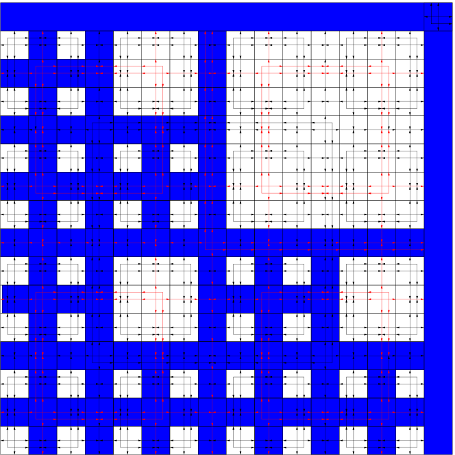
Figure 3.2. Tsirelson’s SFT with entropy dimension $\frac{\log 3}{\log 2}$

Now for a formal description of a more general scheme: Let $2<p$ and $0<q<2p$ be integers. We introduce an extension $Y=Y_{p,q}$ of the SFT $X_{p}$, which has fractional entropy dimension. The tiles will be marked with an extra color which can be blue or white, subject to the restriction specified below.

Choose a subsets

$$B_{h},B_{v}\subset\{0,2,\ldots,p-1\},$$

with $|B_{h}|+|B_{v}|=q$. Impose the restriction that a node $(W,x,y)$ can be marked blue iff $x\in B_{h}$ and $y\in B_{v}$. Further impose the restriction that arrows originating at a blue node must be marked blue, and that whenever an arrow head meets an arrow tail either both must be blue or both not blue. Finally, impose the restriction that whenever a blue arrowhead meets a perpendicular arrow, this arrow must also be blue.

It follows that a node can be blue only if the central node of any cluster containing this node is indexed by $(x,y)\in A^{2}$. Thus, the number of blue nodes in an $n$-cluster is at most $b_{n}=\sum_{k=1}^{n}q^{k}$, so $\log b_{n}\sim n\log q$. Now we allow an extra marking in $\{0,1\}$ for each blue nodes, without any further restrictions. There will be in total $s_{n}=p^{2}\sum_{j=1}^{b_{n}}2^{j}$ $n$-clusters, and so $\log\log s_{n}\sim\log b_{n}\sim n\log q$. Since any admissible $k\ \times k$ configuration in $Y$ is contained in a $(\log_{p}k+1)$-cluster, it follows that

$$\log\log N_{k}(Y)\sim\log\log s_{\log_{p}k}\sim\frac{\log q}{\log(p-1)}\log k.$$

Thus, $Y$ has entropy dimension $\log q/\log(p-1)$.

3.4. SFT with polynomial growth type $2+\frac{\log M}{\log p}$

A different kind of extension for the SFT $X_{p}$ defined in 3.1 will yield an SFT $X_{p,M}\subset\left(S_{p}\times M\right)^{\mathbb{Z}^{2}}$ which has polynomial growth-type $2+\frac{\log M}{\log p}$ for any non-negative integer $M$. The local restrictions will guarantee that the extra marking in $(M)$ is constant within each level, and independent between levels: A white node has the same $(M)$-color as the arrows pointing towards it and away from it, and any arrow has the same $(M)$-marking as its predecessor (at distance $1$ or $2$). An $n$-cluster will have $M^{n}$ possible $(M)$-markings, so $\log N_{p^{k}}(X_{p,T})\sim k(\log M+2\log p)$.

It follows that $P(X_{p,m})=2+\frac{\log M}{\log p}$.

4. The Zheng-Weihrauch hierarchy of real numbers

In order to state our main result, we briefly recall from [16] Weihrauch and Zheng’s hierarchy of real numbers. Denote by $\Gamma_{\mathbb{Q}}$ the set of computable functions $f:\mathbb{N}^{k}\to\mathbb{Q}$ (there exist a Turing machine $\mathcal{R}_{f}$ which terminates with output $f(n_{1},\ldots,n_{k})$, given the input $(n_{1},\ldots,n_{k})\in\mathbb{N}^{k}$). For $n\geq 1$, the classes of real numbers $\Sigma_{n},\Pi_{n}$ and $\Delta_{n}$ are defined as follows:

1. $$\Sigma_{n}:=\{x\in\mathbb{R}:\leavevmode\nobreak\ (\exists f\in\Gamma_{\mathbb{Q}})x=\sup_{i_{1}}\inf_{i_{2}}\ldots\Theta_{i_{n}}f(i_{1},\ldots,i_{n})\}$$

   $$\Pi_{n}:=\{x\in\mathbb{R}:\leavevmode\nobreak\ (\exists f\in\Gamma_{\mathbb{Q}})x=\inf_{i_{1}}\sup_{i_{2}}\ldots\overline{\Theta}_{i_{n}}f(i_{1},\ldots,i_{n})\}$$

2. $\Delta_{n}:=\Sigma_{n}\cap\Pi_{n}$.

In the above $\Theta$ and $\overline{\Theta}$ stand for $\sup$ or $\inf$ according to the parity of $n$.

It is known that for any $n\geq 0$, the inclusions $\Pi_{n}\subset\Sigma_{n+1}$ and $\Sigma_{n}\subset\Pi_{n+1}$ are proper.

In particular, we will be interested in the first few classes in this hierarchy, and some of their equivalent characterizations proved in [16]:

• $x\in\Sigma_{1}$ ($\Pi_{1}$) iff $x=\sup_{n\in\mathbb{N}}f(n)$ ($x=\inf_{n\in\mathbb{N}}f(n)$)

• $x\in\Sigma_{2}$ ($\Pi_{2}$) iff $x=\sup_{n\in\mathbb{N}}\inf_{m\in\mathbb{N}}g(n,m)$ ($x=\inf_{n\in\mathbb{N}}\sup_{m\in\mathbb{N}}g(n,m)$) iff $x=\liminf_{n\to\infty}f(n)$ ($x=\limsup_{n\to\infty}f(n)$).

• $x\in\Delta_{1}$ iff $x=\lim_{n\to\infty}f(n)$ effectively. This means $|f(n)-x|\leq 2^{-n}$.

• $x\in\Delta_{2}$ iff $x=\lim_{n\to\infty}f(n)$.

where $f:\mathbb{N}\to\mathbb{Q}$ and $g:\mathbb{N}^{2}\to\mathbb{Q}$ are computable functions.

This arithmetical hierarchy of real numbers recently already made an appearance in symbolic dynamics. The main result of [7] is that for $d\geq 2$, the class of entropies of ${\mathbb{Z}^{d}}$ SFT’s is $[0,+\infty)\cap\Pi_{1}$. This was followed by a subsequent result of Hochman [6]: For $d\geq 3$, the class of entropies of ${\mathbb{Z}^{d}}$ cellular automata is $[0,+\infty]\cap\Delta_{2}$.

For our purposes, it will be convenient to associate a binary function with a real number in $\Pi_{3}$ (and $\Delta_{2}$, $\Sigma_{2}$):

Lemma 4.1.

1. $x\in[0,1]$ is in $\Pi_{3}$ iff $x$ is the upper-density for some set of integers whose complement is recursively enumerable. In other words, there exists a computable function $g:\mathbb{N}\times\mathbb{N}\to\{0,1\}$ such that

   $$x=\limsup_{n\to\infty}\frac{1}{n}\sum_{k=1}^{n}\inf_{j}g(k,j).$$

2. $y\in[0,1]$ is in $\Sigma_{2}$ iff it is the lower-density of some set of integers whose complement is recursively enumerable. In other words,

   $$y=\liminf_{n\to\infty}\frac{1}{n}\sum_{k=1}^{n}\inf_{j}f(k,j).$$

   For some computable $f:\mathbb{N}\times\mathbb{N}\to\{0,1\}$.

3. $z\in[0,1]$ is in $\Delta_{2}$ iff it is the density of some set of integers whose complement is recursively enumerable. In other words,

   $$z=\lim_{n\to\infty}\frac{1}{n}\sum_{k=1}^{n}\inf_{j}f(k,j).$$

   For some computable $f:\mathbb{N}\times\mathbb{N}\to\{0,1\}$.

Proof.

We prove the part about $x\in\Pi_{3}\cap[0,1]$, as the proofs of the other parts are completely analogous. By [16], for $x$ as above, we have

$$x=\limsup_{n\to\infty}\inf_{j}G(n,j),$$

for some recursive function $G:\mathbb{N}\times\mathbb{N}\to\mathbb{Q}\cap[0,d]$. By replacing $G(n,j)$ with $\min_{k\leq j}G(n,j)$, is a , we can assume that $G$ is monotone in the second variable.

Let $t_{n}=2^{n^{2}}$. We will construct a recursive function $g:\mathbb{N}\times\mathbb{N}\to\{0,1\}$, so that for all sufficiently large integers $n$ and $j$,

(4.1) $$|\frac{1}{t_{n}}\sum_{k=1}^{t_{n}}g(k,j)-G(n,j)|<\frac{1}{n}$$

and for all $l\in(t_{n},t_{n+1})$,

(4.2) $$\frac{1}{l}\sum_{k=1}^{l}g(k,j)=\theta G(n,j)+(1-\theta)G(n+1,j)+\epsilon,$$

for some $\theta\in(0,1)$ and $\epsilon\in(-\frac{1}{n},+\frac{1}{n})$.

This lemma will clearly follow from this.

Here is one way to define the function $g$:

For $(n,j)\in\mathbb{N}^{2}$, let $K_{n,j}:=\lfloor nf(n+1,j)\rfloor$. We thus have $|G(n,j)-K_{n,j}/n|<\frac{1}{n}$. For $t_{n}<k\leq t_{n+1}$, define $g(k,j)=1$ if $(k\mod n)\in\{1,\ldots,K_{n,j}\}$ and $g(k,j)=0$ otherwise. Thus,

$$|\frac{1}{t_{n+1}}\sum_{k=1}^{t_{n+1}}g(k,j)-G(n+1,j)|\leq$$

$$|\frac{1}{t_{n+1}}\sum_{k=1}^{t_{n}}g(k,j)|+\frac{1}{t_{n+1}}\sum_{q=0}^{\frac{t_{n+1}-t_{n}}{n}}|\sum_{r=0}^{n-1}g(nq+r,j)-G(n,j)|+\frac{t_{n}}{t_{n+1}}|G(n,j)|\leq$$

$$\frac{t_{n}}{t_{n+1}}+\frac{n}{t_{n+1}}+\frac{d\cdot t_{n}}{t_{n+1}}<\frac{1}{n}.$$

The last inequality holding for large $n$’s.

A similar estimate shows that equation (4.2) holds.

∎

5. An arithmetical characterization of entropy dimensions of SFTs

5.1. Statement of main theorem

We now have the necessary definitions to state our main result about entropy dimensions of SFTs:

Theorem 5.1.

For any $d\geq 2$,

1. The class of upper entropy dimensions of ${\mathbb{Z}^{d}}$ SFT’s is $[0,d]\cap\Pi_{3}$.

2. The class of lower entropy dimensions of ${\mathbb{Z}^{d}}$ SFT’s is $[0,d]\cap\Sigma_{2}$.

3. The class of entropy dimensions of ${\mathbb{Z}^{d}}$ SFT’s is $[0,d]\cap\Delta_{2}$.

Each of the three statement of theorem 5.1 above splits into two parts. The first part states a necessary restriction on the range of the entropy dimension: For any SFT the upper entropy dimension is a number in $[0,d]\cap\Pi_{3}$. The second part of the statement is a sufficiency claim about this restriction: For any real number $x\in[0,d]\cap\Pi_{3}$ there exists a $\mathbb{Z}^{d}$-SFT $X$ with $\overline{D}(X)=x$.

5.2. Justification of the arithmetical restrictions

For $j\geq k$, let $N_{k,j}(X)$ be the number of $k$-blocks appearing in locally admissible $j$-blocks. It follows that $N_{k}(X)=\inf_{j\geq k}N_{k,j}(X)$. The function $f(k,j)=\frac{\log\log N_{k,j}(X)}{\log k}$ is computable for any SFT $X$. Thus, the upper and lower/ upper entropy-dimensions of any SFT $X$ are of the form $\limsup_{k\to\infty}\inf_{j}f(k,j)$ and $\liminf_{k\to\infty}\inf_{j}f(k,j)$, for a computable function $f:\mathbb{N}^{2}\to\mathbb{Q}$. When the upper and lower entropy dimensions are equal, they are of the form $\lim_{k\to\infty}\inf_{j}f(k,j)$. By [16] numbers of these forms are $\Pi_{3}$, $\Sigma_{2}$ and $\Delta_{2}$ respectively.

The restriction that the entropy dimension of a ${\mathbb{Z}^{d}}$ subshift is in the range $[0,d]$, follows from the fact that for any ${\mathbb{Z}^{d}}$ subshift $X\subset S^{\mathbb{Z}^{d}}$ $N_{k}(X)\leq|S|^{k^{d}}$.

5.3. Construction of SFT with given entropy-dimensions - outline

The proof of the sufficiency part of the claims is constructive in nature: We describe an algorithm, which given a “concrete description” of a number in one of the above classes, returns a $\mathbb{Z}^{d}$-SFT with the appropriate upper/lower entropy dimension.

To simplify the presentation as much as possible, we prove the result for $d=2$. The generalization of the proof to higher dimensions introduces no new difficulties.

By lemma 4.1, this amounts, given a computable function $g:\mathbb{N}^{2}\to\{0,1\}$ to the construction of a $\mathbb{Z}^{2}$ SFT $X$ with

$$\overline{D}(X)=\limsup_{n\to\infty}\frac{2}{n}\sum_{k=1}^{n}\inf_{j}g(j,k)=:\alpha_{1},$$

and

$$\underline{D}(X)=\liminf_{n\to\infty}\frac{2}{n}\sum_{k=1}^{n}\inf_{j}g(j,k)=:\alpha_{2}$$

Here is an overview of this construction: We assume that the function $g$ is given in terms of a Turing Machine $\mathcal{M}$ which computes its value. The SFT $X_{g}$ to be constructed will be set up from $2$ “layers”: a base layer and a control layer. The base layer of $X_{g}$ is essentially of the form $Y_{\alpha_{1},\alpha_{2}}$ from the example in 3.2 above. The control layer is an extension of a $p$-adic SFT from 3.1, where each admissible point represents arbitrarily long partial time-space diagrams of a Turing machine related to $\mathcal{M}$. A maximal sub-configurations of the control-layer which represents a single time-space diagram  is a board. The local restrictions will be set up so that in each of the time-space diagrams represented on a board, the input of the machine corresponds to segments of the base-layer of the point. Admissibility of the point will imply that the machine execution represented in any board does not terminate.

The basic strategy for the construction above was perviously utilized in [7] to construct an SFT with given entropy in $\Pi_{1}\cap[0,\infty)$. Although we bring a self-contained description of construction here, a reader will probably benefit from familiarity with the construction of [7].

The term “boards” in this context, as well as the idea of representing partial time-space diagrams of Turing machine executions goes back to at least to Robinson [12], in his proof of Berger’s theorem.

In some ways controlling the entropy-dimension requires more care than just controlling the topological entropy: We must take care that the growth of the control layer, which represents a time-space diagram  of a Turing machine do not effect the entropy-dimension. We overcome this problem by arranging that boards are very “sparse”, and so will have a negligible effect on the growth of $N_{k}(X_{g})$. For this we use boards which are much sparser then those used in [12] and [7]: In our current construction boards of level $\geq n$ takes up only $o(n^{2})$ cells in a $p^{n}\times p^{n}$ square configuration. Specifically, our boards come in levels, such that boards of level $k$ are translates of a set of the form:

$$\left\{(p^{i},p^{j})\in\mathbb{Z}^{2}:\leavevmode\nobreak\ 0<i,j<k\right\}\cup\{(0,p^{j}):\leavevmode\nobreak\ 0<j<k\}\cup\{(p^{j},0):\leavevmode\nobreak\ 0<j<k\}.$$

This introduces a further difficulty: Machine executions represented in the control layer can only access limited and sparse data from the base layer in order to preform the desired computation. We must balance things so that this “limited data” is sufficient.

Let us turn to the details:

5.4. Sparse representations of Turing machine time-space diagrams

Recall that a Turing machine $\mathcal{M}$ is given by a finite set of Machine states $\Sigma_{S}$ and finite number of tape characters $\Sigma_{T}$, along with a transition function $F:\Sigma_{S}\times\Sigma_{T}\to\Sigma_{S}\times\Sigma_{T}\times\{\leftarrow,\rightarrow\}$, indicating the target state, output character and direction of movent of the machine’s head. A time-space diagram for $\mathcal{M}$ is an array in

$$\left(\Sigma_{S}\cap(\Sigma_{S}\times\Sigma_{T}\times\{\leftarrow,\rightarrow\}\right)^{\mathbb{Z}^{2}},$$

where rows represent a tape configuration and columns represent the evolution of time, in a manner which is consistent with the transition function $F$. Adding to each cell a marking of the direction to the head of the machine in its row (left, or right unless), and including trivial time-space diagram  where the machine’s head never appears, the set of all time-space diagrams for a given Turing machine $\mathcal{M}$ is an SFT.

We now specify our implementation of “boards”:

To begin, we define an SFT $\widehat{X}_{p}$ which extends $X_{p}$ for $p\geq 4$. There will be additional markings on the tiles of $\widehat{X}_{p}$. We call the new labels in $\{r,g,y\}^{2}$, hinting the traffic light colors red, green and yellow. One color label will correspond to the horizontal location and the other corresponds to the vertical location of the node. We will refer to these extra markings as horizontal and vertical traffic-light markings. Boards will consists of nodes with green horizontal and vertical labels. Recall that the position of each node in $X_{p}$ corresponds to a pair of $p$-adic integers. The SFT $\widehat{X}_{p}$ will have the property that yellow (horizontal/vertical) labels appear in nodes whose (horizontal/vertical) position corresponds to a $p$-adic integer which is equal to $(p-1)p^{j}+2p^{k}\mod p^{j+1}$ for some $j\in\mathbb{N}$ and $k<j$. Green (horizontal/vertical) labels will appear in nodes whose (horizontal/vertical) position corresponds to a $p$-adic integer which is equal to $(p-1)p^{j}\mod p^{j+1}$ for some $j\in\mathbb{N}$, and will indicate the bottom and left edges of a board.

The implementation of this is based on a slight generalization of the construction in subsection 3.3. We state this in the following lemma:

Lemma 5.2.

Given $p\geq 2$, a finite set $C$ and a function $A:(p)^{2}\times C\to C$, there is an SFT extension $\widehat{X}_{p}$ of $X_{p}$ such that for ever $x\in\widehat{X}_{p}$ every level-$n$ node with labels $(i,j)\in(p)^{2}$ has a label in $c\in C$, so that $c=A(i,j,c^{\prime})$ where $c^{\prime}\in C$ is the label of the central node of the $n+1$-cluster containing this node.

Proof.

The tiles of $\widehat{X}_{p}$ will be those tiles of $X_{p}$, with an additional marking in $C$ for every tile. The constraints on the additional markings are as follows: an arrow with position labels $(i,j)$ and $C$-marking $c$ can only meet an arrow tail with $C$-marking $c$ or a perpendicular arrow with $C$-marking $c^{\prime}$ satisfying $c=A(i,j,c^{\prime})$. ∎

In our specific example $C=\{r,g,y\}^{2}$, and the function $A$ is of the form $A(i,j,(c_{i},c_{j}))=(F(i,c_{i}),F(j,c_{j}))$ with $F:(p)\times C\to C$ defined by:

1. $F(p-1,c)=g\leavevmode\nobreak\ \forall c\in C$

2. $F(0,g)=g$

3. $F(2,g)=y$

4. $F(i,c)=r\leavevmode\nobreak\ \forall c\in C,i\in(p)\setminus\{0,2,p-1\}$

5. $F(2,y)=r$

It follows from these rules that in any $n$-cluster, the traffic-light markings are determined for those nodes contained in a cluster whose central node has a (vertical/ horizontal) $p$-marking different then $0$ or $2$ contained in more then one cluster which has (vertical/ horizontal) $p$-marking with value $2$. Thus, in a in a $p^{n}\times p^{n}$ configuration of $\widehat{X}_{p}$ which projects onto an $n$-cluster there are only $O(n)$ cells which are not determined. It follows that $N_{k}(\widehat{X}_{p})$ has polynomial bounded-growth.

Level $1$-nodes which have yellow or green traffic-light markings are considered free. Cells with green vertical (respectively horizontal) green traffic-light markings mark the bottom (respectively left) boundary of a board.

In any $n$-cluster, the traffic-light markings are determined for those rows and columns containing a digit different then $\{0,1\}$ or more then $1$ digit which is $1$. Thus,in a in a $p^{n}\times p^{n}$ configuration of $\widehat{X}_{p}$ which projects onto an $n$-cluster there are only $O(n)$ cells which are not determined. It follows that $N_{k}(\widehat{X}_{p})$ has polynomial bounded-growth.

As in [12] and [7], for $x\in\widehat{X}_{p}$, an infinite board is an infinite set $A\subset\mathbb{Z}^{2}$ for which $x\mid_{A}$ represents an infinite time-space diagram  (possibly a trivial one).

The following lemma, summarizes the rest of the “sparse-boards” SFT construction:

Lemma 5.3.

Given integers $p,q\geq 2$ and a Turing machine $\mathcal{M}$ with state set $\Sigma_{S}$ and tape alphabet $\Sigma_{T}$ with $S_{q}\subset\Sigma_{T}$, there exists an extension of $Z=Z_{\mathcal{M},p,q}$ of $\widehat{X}_{p}\times X_{q}$ with the following properties:

1. There are factor maps $\pi_{p}:Z\to\widehat{X}_{p}$ and $\pi_{q}:Z\to X_{q}$.

2. For any point $z\in Z_{\mathcal{M},p,q}$, any board $B$ in $\pi_{p}(z)$ represents a time-space diagram  of $\mathcal{M}$’s execution, with the bottom row of $B$ representing an a configuration of $\mathcal{M}$ in the initial state, with the tape initialized according to the corresponding cells of $\pi_{q}(Z)$.

3. Any any $z\in Z$, no board represents an execution of $\mathcal{R}$ which reaches the terminating state.

4. $N_{k}(Z)$ has polynomial growth.

Proof.

Starting from the SFT $\widehat{X}_{p}\times X_{q}$ we extend it so that every board of level $k$ and will represent a $(k+1)\times(k+1)$ time-space diagram of the Turing machine $\mathcal{M}$: Coordinates belonging both to a free column and a free row will represents cells in this diagram. Free cells will transmit the time-space diagram  information horizontally and vertically whenever there are no obstruction signals, as in [12]. We superimpose the restriction that level $1$-nodes with green horizontal traffic-light markings correspond to the left boundary of the time-space diagram  and tiles with green vertical traffic-light markings correspond to the lower boundary of the time-space diagram . In particular, a level-$1$ node with green horizontal and vertical traffic-light markings represents a Turing machine head in the initial state. We also superimpose restrictions that cells of the bottom row of a board (these are level-$1$ nodes with green vertical traffic-light markings) correspond to the tape initialized according to the corresponding cells of $X_{q}$. The extension of $\widehat{X}_{p}\times X_{q}$ defined in such a way is called is $Z$.

It remains to estimate $N_{k}(Z)$: We already know that $N_{k}(X_{q})=O(k^{2})$ and that $N_{k}(\widehat{X}_{p})$ is bounded by a polynomial. Thus, for a $k\times k$ cube, there are $O(k^{4})$ possibilities for projecting admissible $Z$-configurations onto $X_{p}\times X_{q}$. Once these projections are fixed, it only remains to determine the contents of the time-space diagrams represented in the boards of this configurations. Observe that a time-space diagram of any Turing machine is completely determined by its bottom row. Thus, for all boards of level $\leq\log_{p}k$, the time-space diagrams are determined by the projection onto $X_{q}$ of a slightly larger configuration of size $pk\times pk$. It follows that there are $O(pk^{2})=O(k^{2})$ such configurations. The only part of the configuration which is yet undetermined are those space-time diagrams corresponding to boards of levels $>\log_{p}k$. A most one such board can intersect a $k\times k$ configuration, and no more then $(\log_{p}k)^{2}$ cells of such board can intersect a $k\times k$ square. Thus, the number of possibilities for this space time diagram is bounded from above by $|S|^{\log_{p}k}$ where $S$ is the tape and state alphabet of the Turing machine. This number is polynomial in $k$.

∎

5.5. Completing the construction

By now we have described most of the elements involved in our construction. We now complete the construction. Mainly, we address the problem of preforming the computation of $g$ based on “sparse inputs”:

Lemma 5.4.

Let $g:\mathbb{N}^{2}\to\{0,1\}$ be a recursive function.There exist an SFT $X_{g}$, such that for any $n\in\mathbb{N}$,

$$\max_{x\in X_{g}}|\{(i,j):\leavevmode\nobreak\ 1\leq i,j\leq 2^{k}\leavevmode\nobreak\ x_{i,j}\mbox{ is a blue node}\}|=\prod_{k=1}^{n}4^{a_{k}},$$

where $a_{n}=\inf_{j}g(n,j)$. In addition, $X_{g}$ has the property that $N_{k}(X_{g})$ is bounded by a polynomial in $k$.

Proof.

Choose some odd integer $p>2$ and let $q=2^{p}$.

We build $X_{g}$ as an extension of an SFT of the form $Z_{\mathcal{M},p,q}$ described in lemma 5.3. Recall that $Z_{\mathcal{M},p,q}$ is an extension of $X_{p}\times X_{q}$. Extend this further, by allowing each cross in $X_{q}$ to contain an extra variable $\alpha\in\{0,1\}$. There will be local restrictions which force all $\alpha$ variables corresponding to crosses of the same level to have the same value. As in the example of 3.2, allow nodes and arrows of the $X_{q}$ layer to be blue, enforcing the restriction that blue arrow head must meet blue arrow tail or a blue perpendicular arrow. Also, impose the restriction that a node in $X_{q}$ can be blue only if both its horizontal and vertical labels are even, or if its $\alpha$-variable is equal to $1$. The mechanism of lemma 5.3 will be used to enforce the condition that the $\alpha$-variable is can be set to $1$ only in nodes of levels $n$ for which $a_{n}=1$. This is implemented as follows:

Let $\mathcal{R}$ be a Turing machine which performs the following: First $\mathcal{R}$ evokes the following procedure, which is intended to compute the level $k$ corresponding to the input:

Input: $(x_{n})_{n\in\mathbb{N}}$

1. If $x_{1}$ is not a cross, run indefinitely.

2. Otherwise, find the first $m>1$ such that the horizontal marking of $x_{m+1}$ is not equal to the horizontal marking of $x_{1}$. Set $k=\lceil m\frac{\log p}{\log q}\rceil$.

This procedure indeed finds the desired level $k$, since the condition on $m$ implies that

$$p^{m}<q^{k}\leq p^{m+1},$$

and so

$$m\log p<k\log q\leq(m+1)\log p.$$

Next, $\mathcal{R}$ tries to read the value of the variable $\alpha$ from the input. It is possible if the time-space diagram is on a board in $X_{p}$ which is aligned with the correct parity of the $X_{2}$ layer. Then, if $\alpha=0$, $\mathcal{R}$ runs indefinitely. Otherwise, the machine $\mathcal{R}$ loops over $j=1,2,\ldots$ and terminate iff $g(k,j)=0$ for some $j\in\mathbb{N}$. Clearly, for a cross in level $n$, $\alpha$ can be equal to $1$ only if $a_{n}=1$, and there exists a configuration for which indeed $\alpha=1$ for every cross of level $n$ with $n=1$. ∎

To complete the proof of theorem 5.1, extend the SFT $X_{g}$ to an SFT $Y_{g}$ as follows: Each blue cross an independent head/tail marking. By following the analysis of the example in 3.2, we conclude that

$$\overline{D}(Y_{g})=\limsup_{n\to\infty}\frac{2}{n}\sum_{k=1}^{n}a_{n},$$

and

$$\underline{D}(Y_{g})=\liminf_{n\to\infty}\frac{2}{n}\sum_{k=1}^{n}a_{n}$$

6. Further remarks on growth-type invariants

6.1. Growth-type invariants for topological dynamical systems

The definition of entropy-dimension given in the beginning of this paper is a particular case of a definition given by de Carvalho in [3], which applies to a general action of ${\mathbb{Z}^{d}}$-topological dynamical systems:

Let $(X,T)$ be a ${\mathbb{Z}^{d}}$-dynamical system, e.i $X$ is a compact topological space, $T_{n}:X\to X$ is a homeomorphism for each $n\in{\mathbb{Z}^{d}}$, so that $T_{n}\circ T_{m}=T_{n+m}$ for $n,m\in{\mathbb{Z}^{d}}$. For an open cover $\alpha$, denote by $N(\alpha)$ the cardinality of the smallest sub-covering of $\alpha$. The (upper) entropy dimension of the system is defined by:

$$\overline{D}(X,T)=\inf\left\{s>0:\leavevmode\nobreak\ \sup_{\alpha}\limsup_{n\to\infty}\frac{1}{n^{s}}\log N(\bigvee_{k\in Q_{n}}T_{n}\alpha)=0\right\}$$

Where $Q_{n}=\{1,\ldots,n\}^{d}$, and $\alpha$ ranges over open covers of $X$.

In case $X\subset S^{\mathbb{Z}^{d}}$ is a subshift and $\{T_{n}:\leavevmode\nobreak\ n\in{\mathbb{Z}^{d}}\}$ are the shift maps, the open covering of $X$ by cylinders $\alpha_{0}=\{[s]_{0}:\leavevmode\nobreak\ s\in S\}$ satisfies

$$\limsup_{n\to\infty}\frac{1}{n^{s}}\log N(\bigvee_{k\in Q_{n}}T_{n}\alpha_{0})\geq\limsup_{n\to\infty}\frac{1}{n^{s}}\log N(\bigvee_{k\in Q_{n}}T_{n}\alpha)$$

for every open cover $\alpha$. Thus the $\sup$ over $\alpha$’s can be replaced by taking $\alpha_{0}$.

Now note that for any positive sequence $\{a_{n}\}_{n\geq 0}$, the following holds:

$$\limsup\frac{\log a_{n}}{\log n}=\inf_{\beta\geq 0}\left\{\beta\geq 0:\limsup\frac{a_{n}}{n^{\beta}}>0\right\}$$

The equivalence of the definitions follows from this.

In a similar manner, it is possible to define polynomial growth-type and other growth-type invariants for general dynamical systems.

6.2. Measure-theoretic entropy-dimensions and growth-type invariants

Measure-theoretic counterparts of growth-type invariants such as entropy-dimension have been studied by various authors [2, 5, 8]. In [3] it was shown that for any invariant measure on a topological system the measure-theoretic entropy-dimension is bounded from above by the topological entropy-dimension. Answering a question appearing in [3], Ahn Dou and Park [1] constructed topological systems with positive topological entropy dimension and zero measure-theoretic entropy dimension with respect to any invariant measure. We remark that for the SFTs constructed in the previous section the measure-theoretic entropy dimension is $0$ for any shift-invariant probability measure: For any non-trivial $g$, the density of the blue nodes is $0$ for any point $x\in X_{g}$. It follows that with respect to any invariant probability measure there are (almost) no blue nodes. Thus, the support of any invariant measure is a subshift with polynomial growth, hence the entropy dimension of these subshifts is $0$.

6.3. Growth-type invariants for effectively closed shifts

A subshift $X\subset S^{\mathbb{Z}^{d}}$ is said to be $\Pi_{1}^{0}$ if it is effectively closed - $X$ is the complement of the union of a recursive sequence of basic open neighborhoods. As observed in [14], any SFT is a $\Pi_{1}^{0}$ subshift. The same argument we gave in section 5 shows that for any $\Pi_{1}^{0}$ subshift the upper and lower entropy dimensions are $\Pi_{3}$ and $\Sigma_{2}$ respectively, and the same holds for the polynomial growth types.

6.4. Growth-types for Subactions of SFTs

For any ${\mathbb{Z}^{d}}$ dynamical system a subaction is an action of some subgroup of ${\mathbb{Z}^{d}}$. It is an immediate consequence of the definition that the entropy dimension of a system is greater or equal then the entropy dimension of any subaction.

For algebraic ${\mathbb{Z}^{d}}$-actions, the entropy dimension coincides with the entropy rank - the maximal rank of a subaction with positive entropy. In particular, algebraic SFTs always have integer entropy dimension, which is determined by the entropies of subactions. For algebraic SFTs, the entropy dimension is equal to the Krull dimension of the associated ring. It is also equal to the unique $k\leq d$ such that there is a $k$-dimensional sublattice of ${\mathbb{Z}^{d}}$ for which the action has positive, finite $k$-dimensional entropy. See [4] and related references for details.

For general (non-algebraic) SFTs The presence of a $k$-dimensional subaction with positive,finite entropy does not imply that the entropy dimension is $k$: In [11] it was shown that a certain endomorphism of the $\mathbb{Z}^{2}$-full-shift admits positive, finite entropy. The $\mathbb{Z}^{3}$-subshift obtained from all time-space diagrams of this endomorphism has a $1$-dimensional subaction with finite positive entropy, yet the entropy rank and the entropy dimension are $2$.

In [6] it was shown that any $\Pi_{1}^{0}$-subshift is a isomorphic to a subaction of some higher-dimensional Sofic shift (a factor of an SFT). This result gives useful information on the possibilities of growth-type invariants for subactions of Sofic shifts.

6.5. Polynomial growth types of SFTs

Since

$$\overline{P}(X)=\limsup_{k\to\infty}\inf_{j}\frac{\log N_{k,j}(X)}{\log k},$$

and

$$\underline{P}(X)=\liminf_{k\to\infty}\inf_{j}\frac{\log N_{k,j}(X)}{\log k},$$

with $N_{k,j}(X)$ defined as in section 5, it follows that the upper and lower polynomial growth types are necessarily $\Pi_{3}$ and $\Sigma_{2}$ respectively. Also since $N_{k}(X)$ is a strictly increasing sequence of integers for any infinite subshift, any infinite subshift has polynomial growth order at least $1$. The class of examples in 3.4 shows that the possible values of entropy dimensions are dense in $[2,\infty]$. By a trivial extension of a $\mathbb{Z}$-SFT it is easy to construct a ${\mathbb{Z}^{d}}$-SFT with polynomial growth order $1$.

Using a variation of the construction in section 5 combined with the idea of the example in 3.4, we can prove that any $x\in[4,\infty]$ which is $\Pi_{3}$ (or $\Sigma_{2}$) can be obtained as an upper (or lower) entropy dimension for some $\mathbb{Z}^{2}$ SFT.

To find SFTs with polynomial growth rate in $(1,2)$ seems to require different methods then these in the current paper, since the $p$-adic SFTs themselves have polynomial growth type $2$.

6.6. Number of Periodic Points for SFTs

Let $X$ be a ${\mathbb{Z}^{d}}$ subshift. For any $d$-dimensional lattice $L\subset{\mathbb{Z}^{d}}$, let $P_{L}(X)$ denote the number of fixed points of $X$ under $L$. Unlike $N_{k}(X)$, this is indeed an invariant of $X$. Furthermore, it is a computable invariant: There exists an algorithm which given a set of tiles and a lattice $L$ calculates $P_{L}(X)$ for the SFT associated with these tiles. A naive algorithm of this type will have running time which is exponential in $|\det L|$.

For $k\in\mathbb{N}$ set $P_{k}(X)=P_{k{\mathbb{Z}^{d}}}(X)$.

In dimension $1$, $P_{k}(X)=\mathit{trace}(A^{k})$ for a matrix $A$ associated with $X$. In dimension $d>1$, it is not likely to have a simple formula for $P_{k}(X)$.

It should be possible to prove a lower-bound for the computation time of $P_{k}(X)$ which is exponential in $\log k$:

The problem of determining if a given Turing machine runs into a loop of period $k$ has a lower bound which is exponential in $\log k$. Using SFT representation for time-space diagram  of Turing machines, one can reduce the loop-problem for a Turing machine into counting $L$-periodic points of certain SFTs.

A remarkable paper [9] of Kim, Ormes and Roush gives a simple necessary and sufficient conditions on an $n$-tuple of complex numbers to be the non-zero spectra of a matrix representing an SFT $X$. This gives a relatively simple characterization of the possible sequences $\{P_{k}(X)\}$ for one-dimensional SFTs.

It is interesting to understand the possible asymptotics for $\{P_{k}(X)\}$ when $X$ is an arbitrary multidimensional SFT.

References

• [1] Y.-h. Ahn, D.Β Dou, and K.Β K. Park. Entropy dimensions and variational principle. preprint.
• [2] F.Β Blume. Possible rates of entropy convergence. Ergodic Theory Dynam. Systems, 17(1):45–70, 1997.
• [3] M.Β deΒ Carvalho. Entropy dimension of dynamical systems. Portugal. Math., 54(1):19–40, 1997.
• [4] M.Β Einsiedler, D.Β Lind, R.Β Miles, and T.Β Ward. Expansive subdynamics for algebraic ${\mathbb{Z}}^{d}$-actions. Ergodic Theory Dynam. Systems, 21(6):1695–1729, 2001.
• [5] S.Β Ferenczi and K.Β K. Park. Entropy dimensions and a class of constructive examples. Discrete Contin. Dyn. Syst., 17(1):133–141, 2007.
• [6] M.Β Hochman. On the dynamics and recursive properties of multidimensional symbolic systems. Inventiones Mathematicae, to appear.
• [7] M.Β Hochman and T.Β Meyerovitch. A characterization of the entropies of multidimensional shifts of finite type. Annals of mathematics, to appear.
• [8] A.Β Katok and J.-P. Thouvenot. Slow entropy type invariants and smooth realization of commuting measure-preserving transformations. Ann. Inst. H. PoincarΓ© Probab. Statist., 33(3):323–338, 1997.
• [9] K.Β H. Kim, N.Β S. Ormes, and F.Β W. Roush. The spectra of nonnegative integer matrices via formal power series. J. Amer. Math. Soc., 13(4):773–806 (electronic), 2000.
• [10] D.Β A. Lind. The entropies of topological Markov shifts and a related class of algebraic integers. Ergodic Theory Dynam. Systems, 4(2):283–300, 1984.
• [11] T.Β Meyerovitch. Finite entropy for multidimensional cellular automata. Ergodic Theory Dynam. Systems, 28(1):61–83, 2008.
• [12] R.Β M. Robinson. Undecidability and nonperiodicity for tilings of the plane. Invent. Math., 12:177–209, 1971.
• [13] K.Β Schmidt. Algebraic ideas in ergodic theory, volumeΒ 76 of CBMS Regional Conference Series in Mathematics. Published for the Conference Board of the Mathematical Sciences, Washington, DC, 1990.
• [14] S.Β G. Simpson. Medvedev degrees of 2-dimensional subshifts of finite type. Ergodic Theory and Dynamical Systems, to appear.
• [15] B.Β Tsirelson. A strange two-dimensional symbolic system. unpublished notes from Tel Aviv University math colloquim, 1992.
• [16] X.Β Zheng and K.Β Weihrauch. The arithmetical hierarchy of real numbers. MLQ Math. Log. Q., 47(1):51–65, 2001.