Measuring spin and charge correlations via tunneling-current conductance fluctuations

Abstract

Scanning tunneling miscoscopy is one of the most powerful spectroscopic tools for single-electron excitations. We show that the conductance fluctuations, or noise in the conductance, of a tunneling current into an interacting electron system is dominated by density-density and spin-spin correlations. This allows one to probe two-particle properties (susceptibilities) and collective excitations by standard experimental tunneling methods. We demonstrate this theoretically, using a novel many-body calculation for the multi-center Kondo problem, including both direct and indirect exchange between magnetic atoms. An example of the two-particle correlations around a single magnetic adatom in the Kondo regime, as would be viewed by a scanning tunneling microscope, is given. The spatial dependance of the charge and spin correlations, including the formation of the Kondo cloud in the spin sector, are shown.

Noise spectroscopy, typically current noise, has become an exceedingly useful tool in the study of electronic systems. The intrinsic noise, i.e. the fluctuations of a signal due to inherent uncertainties, generated by an electronic system is not a simple set of random uncorrelated events but contains fundamental information about electron-electron correlations, that is not seen in the (averaged) signal itself. Perhaps, the most well-known demonstration of this was the experimental verification of fractionally charged quasi-particles in the quantum Hall regime, by shot-noise measurements KanePRL94a ; SaminadayarPRL97 . The study of current-current correlations, such as shot-noise or Johnson-Nyquist (thermal) noise, has a long history and has been a prevalent topic of both experimental and theoretical investigations, along with work in related areas, such as conductance fluctuations of mesoscopic wires, mostly by studying the effects of disorder LeePRL85 ; vanOudenaardenPRL97 ; vonOppenPRL97 . Here, we show that in the weak-local-tunneling limit the conductance fluctuations of an unpolarized (spin) current into an interacting system is dominated by density-density correlations or for a spin-polarized current by the spin-spin correlations. This allows one to extract two-particle characteristics from tunneling experiments along with single-particle quantities, such as the density of states or magnetization. Macroscopic two-particle properties, like the compressibility or magnetic susceptibility, are easily measurable. However, few if any techniques exists to measure these quantities at a local microscopic scale, with spatial and energy resolution. For instance, almost fifty-years after the discovery and theoretical explanation of the Kondo effect, the spatially localized spin correlations around a magnetic impurity—the Kondo cloud—has never been experimentally observed.

The atomic spatial resolution of a scanning tunneling microscope (STM) makes it a natural choice to study local fluctuations on the microscopic scale. This combination of an STM and noise spectroscopy has already been used to develop the field of electron spin resonance scanning tunneling microscopy (ESR-STM)ManassenPRL89 . With a similar experimental setup in mind we will limit ourselves to an STM system, along with making the common approximations, such as weak local tunneling and where the STM is assumed to be a weakly or non-correlated Fermi liquid with a featureless single-particle density of states. Although, the work presented here is with reference to an STM, the results are not limited to such systems and are valid anywhere such approximations can be made.

The total Hamiltonian is taken to be

$$H=H_{\rm STM}+H_{\rm sub}+H_{\rm tun},$$

where $H_{\rm sub}$ is the general interacting Hamiltonian of the substrate and $H_{\rm STM}=\sum_{{\bf k}\sigma}(\epsilon_{{\bf k}\sigma}-\mu-eV)a^{\dagger}_{{\bf k}\sigma}a_{{\bf k}\sigma}$ is the Hamiltonian of the STM. As usual, we assume that the STM is a noninteracting Fermi system with an energy independent density of states near the Fermi energy $\epsilon_{\rm F}=\mu$. This is an optimal condition for spectroscopic aims. The chemical potential of the STM is displaced by $eV$, where the charge of the electron is $-e$ and $V$ is the applied voltage. The tunneling is determined by $H_{\rm tun}=\sum_{{\bf k},{\bf k}^{\prime},\sigma}\big{[}{\rm T}a^{\dagger}_{{\bf k}\sigma}b_{{\bf k}^{\prime}\sigma}+{\rm H.c.}\big{]}$, with tunneling amplitude ${\rm T}$, which is assumed to be independent of momenta ${\bf k},{\bf k}^{\prime}$. The operators $b^{\dagger}_{{\bf k}^{\prime}\sigma}$ and $b_{{\bf k}^{\prime}\sigma}$ are the mode creation and annihilation operators for the substrate. The current operator is defined as $\hat{I}=-e\partial_{t}{\hat{N}}_{\rm STM}$, where ${\hat{N}}_{\rm STM}=\sum_{{\bf k}\sigma}a^{\dagger}_{{\bf k}\sigma}a_{{\bf k}\sigma}$ is the particle number operator for the STM. Assuming $\big{[}{\hat{N}}_{\rm STM},H_{\rm sub}\big{]}=0$, by Heisenberg’s equation of motion, $\hat{I}=ie\big{[}{\hat{N}}_{\rm STM},H_{\rm tun}\big{]}$ (with $\hbar=1$). Evaluating the commutator using $\big{\{}a_{{\bf k}\sigma},b^{\dagger}_{{\bf k}^{\prime}\sigma^{\prime}}\big{\}}=0$ leads to, within the tunneling Hamiltonian formalism, the common expression for the current operatorMahanbook

$${\hat{I}}=ie\sum_{\sigma}\sum_{{\bf k},{\bf k}^{\prime}}\big{[}{\rm T}a^{\dagger}_{{\bf k}\sigma}b_{{\bf k}^{\prime}\sigma}-{\rm H.c.}\big{]}.$$ (1)

To obtain the experimentally measured current, one needs to obtain the non-equilibrium expectation value of (1). We do this within the linear response (LR) regime, treating the tunneling as the perturbation and assuming the STM and substrate are separately in thermodynamic equilibrium. If the system is decoupled in the infinite past, $t=-\infty$, the current operator within LR is given as

$$\hat{I}_{\rm LR}(t)=\hat{I}+i\int\limits_{-\infty}^{t}dt^{\prime}\,\big{[}H_{\rm tun}(t^{\prime}),{\hat{I}}(t)\big{]},$$ (2)

where $\hat{O}(t)=e^{iH_{0}t}\hat{O}e^{-iH_{0}t}$ and $H_{0}=H_{\rm STM}+H_{\rm sub}$. The expectation value of (2) with respect to $H_{0}$, $\big{<}\hat{I}_{\rm LR}\big{>}_{H_{0}}={\rm Tr}\,\hat{I}_{\rm LR}e^{-\beta H_{0}}/{\rm Tr}\,e^{-\beta H_{0}}$, gives the current to leading order in the tunneling amplitude, $T$. Therefore, the linear conductance, in this approximation, is given by $G_{\rm LR}=\partial_{V}\big{<}\hat{I}_{\rm LR}\big{>}_{H_{0}}$. Assuming that the expectation value and derivative commute, a conductance operator can also be defined by $\hat{G}_{\rm LR}=\partial_{V}\hat{I}_{\rm LR}$ (see supplemental material for details). With an operator expression for the conductance, one can obtain the fluctuations or specifically the spectral density of the conductance, defined as

$$S({\bf r},\omega) =\frac{1}{2}\int dt\,e^{i\omega t}\big{<}\big{\{}\delta\hat{G}_{\rm LR}({\bf r},t),\delta\hat{G}_{\rm LR}({\bf r},0)\big{\}}\big{>}_{H_{0}},$$ (3)

where $\delta\hat{G}_{\rm LR}=\hat{G}_{\rm LR}-\big{<}\hat{G}_{\rm LR}\big{>}$. The low-temperture zero-frequency limit of (3) can be shown to be given by

$$S({\bf r},\omega=0) =\pi^{2}e^{4}|{\rm T}|^{4}\big{[}\rho_{\rm STM}(eV)\big{]}^{2}\chi^{\rm ch}_{\rm sub}({\bf r},\omega=0)$$

$$+32\pi^{2}e^{4}|{\rm T}|^{4}\big{[}m_{\rm STM}(eV)\big{]}^{2}\chi^{\rm sp}_{\rm sub}({\bf r},\omega=0),$$ (4)

with $\rho_{\rm STM}=\sum_{\sigma}\rho^{\sigma}_{\rm STM}$, $m_{\rm STM}=\rho^{\uparrow}_{\rm STM}-\rho^{\downarrow}_{\rm STM}$, and

$$\chi^{\rm ch}_{\rm sub}({\bf r},t) =\big{<}\delta\hat{n}({\bf r},t)\delta\hat{n}({\bf r},0)\big{>}_{H_{\rm sub}}$$ (5a)

$$\chi^{\rm sp}_{\rm sub}({\bf r},t) =\big{<}\hat{s}^{z}({\bf r},t)\hat{s}^{z}({\bf r},0)\big{>}_{H_{\rm sub}},$$ (5b)

where $\chi^{\rm ch}_{\rm sub}$ and $\chi^{\rm sp}_{\rm sub}$ are the local charge- and spin-susceptibilities respectively, with density and spin-density operators of the substrate $\hat{n}$ and $\hat{s}^{z}$. The compressibility (5a) is given in terms of the density variation; $\delta\hat{n}=\hat{n}-\left<\hat{n}\right>$. The extension of equation (Measuring spin and charge correlations via tunneling-current conductance fluctuations) to non-zero frequency is in principle straightforward, although relating the finite-frequency results to physically meaningful quantities is not. This is analogous to the standard current shot-noise result, where it is only the zero-frequency component of the noise that is directly proportional to the measured current. Equation (Measuring spin and charge correlations via tunneling-current conductance fluctuations) in itself may not be surprising as, loosely speaking, the conductance is determined by a single-particle correlation function (the density of states), thus for a conductance-conductance correlation one could expect two-particle quantities. As a result one can obtain local susceptibilities, as a function of position, using only a single STM or current probe.

It should also be noted that, in the weak tunneling limit the standard expression for the current noise, which is given by the current-current correlation function, leads to the well-known shot-noise relation. The zero-frequency shot noise is proportional to the current itself which goes as the tunneling amplitude squared, while (Measuring spin and charge correlations via tunneling-current conductance fluctuations) is proportional to $|{\rm T}|^{4}$. This seemingly contridictory result is explained by the fact that in general the complete characterization of fluctuations or noise of any signal is not determined solely by a second-order moment, such as a current-current correlation (variance), but by all higher moments as well. For instance one could obtain a similar result to equation (Measuring spin and charge correlations via tunneling-current conductance fluctuations) from the current signal itself, by a suitable choice of a current-current-current-current correlation (kurtosis). Also, in any real experimental measurement, the tunneling amplitude enters the tunneling current to all orders. These higher order terms, the so-called vertex corrections, to the tunneling are small, and they are typically neglected; although recent STM experimentsHirjibehedinScience06 ; HeinrichScience04 ; HeinrichScience02 have shown they can lead to detectable contributions. For example, the single-triplet transition (which appears in the spin-susceptibility but not in the single-particle density of states) of an atomic spin chain has been observed. As yet no full theoretical description of these effects exists, for one has to go beyond the standard tunneling Hamiltonian approximationsPrangePR63 to describe the experimental $\partial^{2}_{V}\big{<}\hat{I}(eV)\big{>}$ curves. Such a formulation, relating these vertex corrections to physical quantities, like spin or charge susceptibilities, is highly desirable and is of ongoing interest.

As can be seen from (Measuring spin and charge correlations via tunneling-current conductance fluctuations), for a non-magnetic STM, i.e $m_{\rm STM}=0$, the charge susceptibility (5a) determines the fluctuations, while for a spin-polarized STM (SP-STM), $m_{\rm STM}\neq 0$, the spin susceptibility (5b) would be expected to dominate. This is analogous to standard SP-STM measurements, where the magnetic structure of the substrate is easily resolved, even for relatively small spin polarization WortmannPRL01 ; HeinzeScience00 . Among the many possibilities, one could spatially resolve the low-energy spin correlations near one or more Kondo impurities, where the geometry of the nano-cluster, as well as the direct and indirect exchange processes between atoms are in strong competitionSavkinPRL05 with the Kondo correlations, see Fig. 1. Here, as a simple but intriguing example, we show that one can explore the localized spin correlations around a single magnetic atom, the so-called Kondo cloud. We now turn to a calculation of the local susceptibilities (5a) and (5b) for such a system.

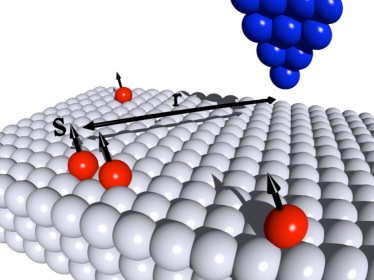
Figure 1: STM setup. Schematic of an STM and several magnetic impurities with spin ${\bf S}$ on a non-magnetic surface. Exchange between the magnetic atoms can be indirect, though the substrate, or if in close proximity, directly by the overlap of impurity wave functions. Normally, the Kondo effect is probed by tunneling into a single impurity or nano-cluster, i.e. ${\bf r}\approx 0$, where the formation of a Fano-lineshape in the current(conductance)-voltage curve is observed.

The Kondo effect has been extensively studied both theoretically and experimentally Hewson , more recently by using an STM to image single or multiple magnetic adatoms on a metallic surface LiPRL98 ; MadhavenScience98 ; KnorrPRL02 ; NagaokaPRL02 ; WahlPRL04 ; NeelPRL2007 , e.g. Fig.1. Experimentally, for the most part, attention has been restricted to measuring the formation of the Abrikosov-Suhl-Kondo resonance of the density of states, while in the Kondo regime. Theoretically many other quantities have been explored, such at the non-local correlations between the impurity and conduction electron, which is typically used to define and determine the Kondo screening length $\xi_{\rm K}$. To calculate the required bath correlation functions (5a) and (5b), in the presence of magnetic impurities, we used a numerically exact scheme, briefly outlined below (see supplementary information for details). In principle this formalism allows one to calculate all physical quantities including those of the impurities, the bath, and all $n$-particle correlations. Although straightforward and when applied recovers known results SantoroPRB91b ; PollweinZPhysB88 ; IshiiJLTP78 ; BordaPRB07b , to our knowledge it has not appeared in the literature. We believe this is the ideal method to apply to real experimental systems. Especially those involving multi-impurities, in close proximity, where exchange between atoms, direct and indirect, or even the overlapping and interference of individual Kondo clouds, becomes important.

The most general Hamiltonian of a noninteracting substrate with $n$-bands coupled to $N$-atomic impurities with amplitude $V^{n}_{{\bf k}\sigma,\alpha s}$, and including direct exchange $J_{\alpha,\alpha^{\prime}}$ between impurities is

$$H_{\rm sub}=\sum_{n}\sum_{\bf k,\sigma}(\epsilon^{n}_{{\bf k}\sigma}-\mu)b^{\dagger}_{n,{\bf k}\sigma}b_{n,{\bf k}\sigma}+\sum_{\alpha=1}^{N}\sum_{s}E_{\alpha s}c^{\dagger}_{\alpha s}c_{\alpha s}$$

$$+\frac{1}{2}\sum_{\alpha=1}^{N}\sum_{s_{1}\cdots s_{4}}U^{\alpha}_{s_{1}\cdots s_{4}}c^{\dagger}_{\alpha s_{1}}c^{\dagger}_{\alpha s_{2}}c_{\alpha s_{3}}c_{\alpha s_{4}}+\frac{1}{2}\sum_{\alpha\neq\alpha^{\prime}}^{N}J_{\alpha,\alpha^{\prime}}{\hat{\bf S}}_{\alpha}\cdot{\hat{\bf S}}_{\alpha^{\prime}}$$

$$+\sum_{\alpha=1}^{N}\sum_{n}\sum_{{\bf k},\sigma,s}\big{[}V^{n}_{{\bf k}\sigma,\alpha s}b^{\dagger}_{n,{\bf k}\sigma}c_{\alpha s}+{\rm H.c.}\big{]},$$ (6)

where $c^{\dagger}_{\alpha s}$ $(c_{\alpha s})$ is the electron creation (annihilation) operator for an impurity, with a complete set of quantum numbers $s$. Here ${\hat{\bf S}}_{\alpha}$ is the total spin of an adatom, $E_{\alpha s}$ are the bare energy levels, and $U^{\alpha}_{s_{1}\cdots s_{4}}$ the Coulomb interaction. In principle all of the above parameters, along with the dispersion of the metal $\epsilon^{n}_{{\bf k}\sigma}$, could be obtained from an ab initio calculation, e.g. density functional theory. With respect to the Hamiltonian, equation (Measuring spin and charge correlations via tunneling-current conductance fluctuations), the generating functional, with action $S_{A},$ for the entire system can be written as a functional integral over Grassmann variables, including source terms $A_{i}$ and $\bar{A}_{i}$ for the bath electrons and each impurity; ${Z}_{A}=\int D[\bar{c},c]D[\bar{b},b]e^{-S_{A}}$. Because the host metal is assumed to be noninteracting, i.e. Gaussian, the bath electrons can be integrated out exactly, leading to a reduced generating functional ${Z}_{A}\sim\int D[\bar{c},c]e^{-S^{\rm eff}_{A}}$, with an effective action (Hamiltonian) for the impurity sites. The propagator of the bath or any correlation function can be obtain by suitable functional differentiation of the effective action with respect to the sources. Doing so, the only unknown correlators are those of the impurities. The evaluation of which can be done using a variety of computationally fast and accurate impurity solvers. Here, we used the numerically exact continuous-time quantum Monte Carlo (CT-QMC) method of Ref. [RubtsovPRB05, ].

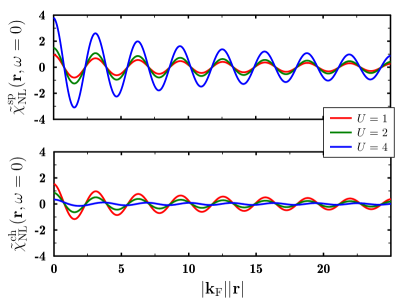
Figure 2: Non-local impurity-bath correlations. The zero-frequency non-local (NL) spin (top) and charge (bottom) correlations, defined as $\chi^{\rm sp}_{\rm NL}({\bf r},t)=\big{<}\hat{s}^{z}({\bf r},t)\hat{S}^{z}_{\rm imp}(0)\big{>}$ and $\chi^{\rm ch}_{\rm NL}({\bf r},t)=\big{<}\delta\hat{n}({\bf r},t)\delta\hat{N}_{\rm imp}(0)\big{>}$, between a magnetic impurity and the conduction electrons as a function of distance from the impurity. In the graph $\tilde{\chi}_{\rm NL}=\frac{2|{\bf k}_{\rm F}|^{2}|{\bf r}|^{2}}{\pi N_{\sigma}\Gamma}\chi_{\rm NL}$. All other relevant parameters are given in Table 1.

$\epsilon_{\rm F}$		$E_{c}$		$U$	$T_{\rm K}$	$\xi_{\rm K}$
6.0		-0.5		1.0	0.168	$\sim$ 70
6.0		-1.0		2.0	0.0865	$\sim$ 140
6.0		-2.0		4.0	0.0216	$\sim$ 555

Table 1: Parameters for the symmetric single-impurity spin-$1/2$ Anderson model in energy units of $\Gamma=\pi|V|^{2}N_{\sigma}({\epsilon}_{\rm F})$, where $\epsilon_{\rm F}$ and $N_{\sigma}({\epsilon}_{\rm F})$ are the Fermi energy and spin-resolved noninteracting density of states of the bath respectively. Lengths are in units of the inverse Fermi wavevector $|{\bf k}_{\rm F}|^{-1}$. The Kondo temperature $T_{\rm K}$ is obtained from the Bethe-Ansatz solution WiegmannJPhysC83a . The expected size of the Kondo screening cloud is of order $\xi_{\rm K}\approx\hbar v_{\rm F}/(k_{\rm B}T_{\rm K})$, where $v_{\rm F}$ is the Fermi velocity. Unless otherwise stated all calculations were done at an inverse-temperature of $(k_{\rm B}T)^{-1}=\beta=200$, well below the Kondo temperature for these parameters.

As an example of the usefulness and flexibility of the above formalism, we calculated the zero-frequency non-local charge and spin correlations between an impurity and the bath (Fig. 2), which has been extensively studied both analytically and numerically for equal timesIshiiJLTP78 ; PollweinZPhysB88 ; GubernatisPRB87 ; SorensenPRB96 ; BordaPRB07 , i.e. $t=0$. For simplicity and clarity, the real Hamiltonian (Measuring spin and charge correlations via tunneling-current conductance fluctuations) is approximated by the symmetric single-impurity spin-$1/2$ Anderson model Hewson , with an onsite $U$ and a 3D parabolic dispersion for the bath. We will also neglect the direct tunneling into the impurity. With this contribution our results would be modified only for ${\bf r}\approx 0$. In the low-energy or low-frequency regime, Fig. 2 clearly shows a separation of scales between spin and charge correlations as the on-site Coulomb energy $U$ is increased, as compared to the case of equal times (effectively high-energy), e.g. Ref. [GubernatisPRB87, ]. This is what one would expect as the dominate correlations of the Kondo effect are at low energy, while charge fluctuations of the impurity are suppressed with increasing $U$.

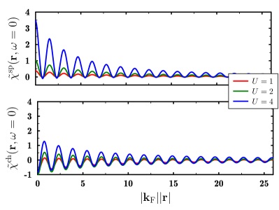
Figure 3: Local correlations of the bath. The zero-frequency local spin (top) and charge (bottom) susceptibilities, equations (5a) and (5b), of the bath for the single-impurity spin-$1/2$ Anderson model as a function of the distance from the impurity site. Here, $\tilde{\chi}=\big{[}\frac{2\Gamma|{\bf k}_{\rm F}||{\bf r}|}{\pi N_{\sigma}}\big{]}^{2}\chi$. All parameters are the same as in Fig. 2 and are given in Table 1.

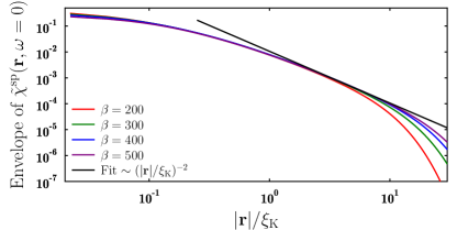
Figure 4: Envelope of spin-spin correlation. The envelope of the zero-frequency local spin susceptibility (equation (5b), shown in Fig. 2) for fixed $U=1$ and different temperatures $T$; $\beta=(k_{\rm B}T)^{-1}$. The horizontal axis has been rescaled by the Kondo length; $\xi_{\rm K}=\hbar v_{\rm F}/(k_{\rm B}T_{\rm K})$. All other parameters are given in Table 1.

In Fig. 3 the zero-frequency local charge and spin susceptibilities of the bath [equations (5a) and (5b)], which determine the conduction fluctuations, for different $U$ are shown. The oscillation period of both is $\pi/2$, the same as Friedel oscillations, but the spin correlation function is $\pi/2$ phase shifted from that of the charge. The envelope or decay of the spin correlations as a function of distance is shown in Fig. 4. For ${\bf r}\ll\xi_{\rm K}$ the correlations show a non-algebraic decay, which changes to a power-law for ${\bf r}\approx\xi_{\rm K}$, and ultimately, at finite temperature, the correlations are exponentially cut-off by the thermal length $\xi_{T}\sim\hbar v_{\rm F}/k_{\rm B}T$. The appearance of the thermal length can be seen for the largest values of ${\bf r}$ in Fig. 4, as the power-law changes over into an exponential. At zero-temperature the decay would remain a power-law for ${\bf r}\gg\xi_{\rm K}$. The simple physical interpretation of this is: at zero-temperature the magnetic impurity is almost fully screened by conduction electrons within $\xi_{\rm K}$, thus outside of this length scale correlations are weak and decay quite rapidly, but within $\xi_{\rm K}$ correlations of the bath, mediated by the impurity, remain non-trivial.

In conclusion we have shown that the conductance fluctuations of a tunneling current into an interacting system is determined by the charge and spin susceptibilities of the system. We have also shown that one application of this is to use an SP-STM to detect the Kondo screening length, $\xi_{\rm K}$, for a magnetic adatom on a metallic surface. Although the Kondo problem has been and continues to be one of the most intensively studied phenomena in condensed matter physics, there has yet to be an experimental conformation of this theoretical prediction concerning the screening cloud. We have furthermore developed a general method to exactly calculate $n$-point correlations for experimentally relevant setups consisting of multiple adatoms or correlated “sites”. Extension of these results to superconducting systems and quantum dot geometries is of future interest.

SUPPLEMENTARY INFORMATION

SI Conductance operator and spectral density

Quantum mechanically the fluctuations, or uncertainty, of an observable is related to the variance of its expectation value. To obtain an expression for the conductance fluctuations or more specifically the spectral density, one needs an operator for the conductance. This can be found by taking the derivative of the linear response expression of the tunneling current, equation (2), with respect to the applied voltage, $V$. Doing so gives

$$\hat{G}_{\rm LR}({\bf r},t) =ie^{2}|{\rm T}|^{2}\sum_{\sigma,\sigma^{\prime}}\int\limits_{-\infty}^{\infty}dt^{\prime}\,\Theta(t-t^{\prime})(t-t^{\prime})\Big{\{}\big{[}C_{\sigma^{\prime}}({\bf r},t^{\prime}),C^{\dagger}_{\sigma}({\bf r},t)\big{]}-\big{[}C_{\sigma}({\bf r},t),C^{\dagger}_{\sigma^{\prime}}({\bf r},t^{\prime})\big{]}\Big{\}}$$

$$-ie^{2}|{\rm T}|^{2}\sum_{\sigma,\sigma^{\prime}}\int\limits_{-\infty}^{\infty}dt^{\prime}\,\Theta(t-t^{\prime})(t+t^{\prime})\Big{\{}\big{[}C_{\sigma}({\bf r},t),C_{\sigma^{\prime}}({\bf r},t^{\prime})\big{]}+\big{[}C^{\dagger}_{\sigma}({\bf r},t),C^{\dagger}_{\sigma^{\prime}}({\bf r},t^{\prime})\big{]}\Big{\}},$$ (SI.1)

where $C_{\sigma}({\bf r})$ is defined in terms of the field operators of the STM and substrate; $C_{\sigma}({\bf r})=\Psi^{\dagger}_{\rm STM}({\bf r}\sigma)\Psi_{\rm sub}({\bf r}\sigma)$. Although the tunneling matrix elements, $\rm T$, in (SI) have different dimensions than that of (1), we will use the same symbol for simplicity. Upon taking the expectation value, the second term of (SI) generates anomalous Green’s functions that only contribute for a supercurrent. These terms are responsible for the Josephson effect and will not be considered here. For a non-superconducting system the expectation of (SI) recovers the well-known expression for the conductance in terms of the local single-particle density of states $\rho^{\sigma}({\bf r},\omega)$; $\big{<}\hat{G}_{\rm LR}\big{>}_{H_{0}}=2\pi e^{2}|{\rm T}|^{2}\sum_{\sigma}\rho^{\sigma}_{\rm STM}(\epsilon_{\rm F})\rho^{\sigma}_{\rm sub}({\bf r},eV)$.

The symmetrized spectral density that characterizes the frequency distribution of fluctuations of the conductance about its averaged value is defined as

$$S({\bf r},\omega) =\frac{1}{2}\int dt\,e^{i\omega t}\big{<}\big{\{}\delta\hat{G}_{\rm LR}({\bf r},t),\delta\hat{G}_{\rm LR}({\bf r},0)\big{\}}\big{>}_{H_{0}},$$ (SI.2)

where $\delta\hat{G}_{\rm LR}=\hat{G}_{\rm LR}-\big{<}\hat{G}_{\rm LR}\big{>}$. This expression for the spectral density assumes time-translational invariance, although the full expression for the conductance operator (SI) contains non time-translational invariant terms, these vanish for non-superconducting systems. Using (SI) and (SI.2), a lengthy, but straightforward, calculation (SI.2) gives the zero-frequency component of the noise as

$$S({\bf r},\omega=0) =8\pi^{2}e^{4}|{\rm T}|^{4}\big{[}\rho_{\rm STM}(eV)\big{]}^{2}\chi^{\rm ch}_{\rm sub}({\bf r},\omega=0)+32\pi^{2}e^{4}|{\rm T}|^{4}\big{[}m_{\rm STM}(eV)\big{]}^{2}\chi^{\rm sp}_{\rm sub}({\bf r},\omega=0).$$ (SI.3)

Equation (SI.3) is the starting point and motive for the remaining calculations and results of the article. Technically, only the vertex corrections of (5a) and (5b) are measured in (SI.3), but in the low-temperature limit, the single-particle contribution to these correlation functions is negligible and vanishes at zero temperature. Thus, we will work with the full correlation functions for simplicity and clarity.

SII Generating functional for N-correlated sites

In this section we show how one can, in a simple and straightforward manner, obtain arbitrary correlation functions of a system consisting of $N$-correlated sites in contact with a non-interacting bath. In essence this method reduces all correlations to correlations involving only the impurity operators. The remaining impurity problem can then be solved using a variety of techniques, such as numerical renormalization group or quantum Monte Carlo. Theoretically the number of impurities $N$ can be arbitrary, but in practice it is limited by the complexity of the system at hand, such as the number of bands of the substraight and orbitals of the adatoms. In the simplest case, for two-particle properties, an upper bound of four or five Anderson impurities could be incorporated using the CT-QMC impurity solver used in this work.

The partition function $Z={\rm Tr}\,e^{-\beta H}$ with respect to the $N$-impurity Hamiltonian (Measuring spin and charge correlations via tunneling-current conductance fluctuations) can be written as a functional integral over Grassmann fields (by inserting complete sets of fermionic coherent states) as

$$Z=\prod_{\alpha=1}^{N}\int{D}[\bar{b},{b}]{D}[\bar{c}_{\alpha},{c}_{\alpha}]e^{-S}$$ (SII.1)

with an action $S$ in Fourier-space

$$S =\sum_{n}\sum_{{\bf k}\sigma}\sum_{i\omega_{m}}\bar{b}^{n}_{{\bf k}\sigma}(i\omega_{m})\big{[}i\omega_{m}-(\epsilon^{n}_{{\bf k}\sigma}-\mu)\big{]}{b}^{n}_{{\bf k}\sigma}(i\omega_{m})+\sum_{\alpha,s}\sum_{i\omega_{m}}\bar{c}_{\alpha s}(i\omega_{m})(i\omega_{m}-E_{\alpha s}){c}_{\alpha s}(i\omega_{m})$$

$$+\sum_{n,\alpha,s}\sum_{{\bf k}\sigma}\sum_{i\omega_{m}}\big{[}V^{n}_{{\bf k}\sigma,\alpha s}\bar{b}^{n}_{{\bf k}\sigma}(i\omega_{m}){c}_{\alpha s}(i\omega_{m})+V^{*n}_{{\bf k}\sigma,\alpha s}\bar{c}_{\alpha s}(i\omega_{m}){b}^{n}_{{\bf k}\sigma}(i\omega_{m})\big{]}+S_{\rm int}[\bar{c}_{\alpha s}(i\omega_{m}),{c}_{\alpha s}(i\omega_{m})],$$ (SII.2)

where $i\omega_{m}$ are fermionic Matsubara frequencies and $S_{\rm int}$ is the term of the action (Hamiltonian) that corresponds to the interactions of the $N$ impurities. The actual form of which is immaterial, as long as it is a local interaction. By introducing Grassmann source terms, $A$ and $\bar{A}$ for each impurity and the bath electrons, the generating functional $Z_{A}$ for the system is given by

$$Z_{A}=\prod_{\alpha=1}^{N}\int{D}[\bar{b},{b}]{D}[\bar{c}_{\alpha},{c}_{\alpha}]e^{-S}\exp \bigg{\{}\sum_{\alpha,s}\sum_{i\omega_{m}}\big{[}\bar{A}_{\alpha s}(i\omega_{m}){c}_{\alpha s}(i\omega_{m})+{A}_{\alpha s}(i\omega_{m})\bar{c}_{\alpha s}(i\omega_{m})\big{]}$$

$$+\sum_{n}\sum_{{\bf k}\sigma}\sum_{i\omega_{m}}\big{[}\bar{A}^{n}_{{\bf k}\sigma}(i\omega_{m}){b}^{n}_{{\bf k}\sigma}(i\omega_{m})+{A}^{n}_{{\bf k}\sigma}(i\omega_{m})\bar{b}^{n}_{{\bf k}\sigma}(i\omega_{m})\big{]}\bigg{\}}.$$ (SII.3)

Because we have assumed a non-interacting bath and local interactions of the impurities, the bath electrons remain Gaussian and with the identity

$$\int D[\bar{\eta},\eta]\exp\Big{[}{-\iint dxdx^{\prime}\bar{\eta}(x)M(x,x^{\prime})\eta(x^{\prime})+\int dxJ(x)\bar{\eta}(x)}{\xi}(x)+\int dxJ^{*}(x)\bar{\xi}(x)\eta(x)\Big{]}$$

$$=\det[M(x,x^{\prime})]\exp\Big{[}\iint dxdx^{\prime}J^{*}(x){\bar{\xi}}(x)M^{-1}(x,x^{\prime}){\xi}(x^{\prime})J(x^{\prime})\Big{]},$$ (SII.4)

can be exactly integrated out of the generating functional (SII), leading to

$$Z_{A}=\det\big{[}i\omega_{m}-(\epsilon^{n}_{{\bf k}\sigma}-\mu)\big{]}\prod_{\alpha=1}^{N}\int{D}[\bar{c}_{\alpha},{c}_{\alpha}]e^{-S_{\rm eff}}\exp\Bigg{\{}\sum_{\alpha,s}\sum_{i\omega_{m}}\big{[}\bar{A}_{\alpha s}(i\omega_{m}){c}_{\alpha s}(i\omega_{m})+{A}_{\alpha s}(i\omega_{m})\bar{c}_{\alpha s}(i\omega_{m})\big{]}$$

$$+\sum_{n,\alpha,s}\sum_{{\bf k}\sigma}\sum_{i\omega_{m}}\frac{V^{n}_{{\bf k}\sigma,\alpha s}{c}_{\alpha s}(i\omega_{m})\bar{A}^{n}_{{\bf k}\sigma}(i\omega_{m})}{i\omega_{m}-(\epsilon^{n}_{{\bf k}\sigma}-\mu)}+\sum_{n,\alpha,s}\sum_{{\bf k}\sigma}\sum_{i\omega_{m}}\frac{{A}^{n}_{{\bf k}\sigma}(i\omega_{m})V^{*n}_{{\bf k}\sigma,\alpha s}\bar{c}_{\alpha s}(i\omega_{m})}{i\omega_{m}-(\epsilon^{n}_{{\bf k}\sigma}-\mu)}+\sum_{n}\sum_{{\bf k}\sigma}\sum_{i\omega_{m}}\frac{A^{n}_{{\bf k}\sigma}(i\omega_{m})\bar{A}^{n}_{{\bf k}\sigma}(i\omega_{m})}{i\omega_{m}-(\epsilon^{n}_{{\bf k}\sigma}-\mu)}\Bigg{\}},$$ (SII.5)

where the effective action of the impurities is, in matrix notation,

$$S_{\rm eff}=-\sum_{s,s^{\prime}}\sum_{i\omega_{m}}{\bf\bar{c}}^{T}_{s}(i\omega_{m}){\bf{\cal G}_{0}^{-1}}(i\omega_{m}){\bf{c}}_{s^{\prime}}(i\omega_{m})+S_{\rm int}[\bar{c}_{\alpha s}(i\omega_{m}),{c}_{\alpha s}(i\omega_{m})]$$ (SII.6)

with

$${\bf\bar{c}}_{s}(i\omega_{m})=\left(\begin{array}[]{c}\bar{c}_{s\alpha=1}(i\omega_{m})\\ \vdots\\ \bar{c}_{s\alpha=N}(i\omega_{m})\end{array}\right),\hskip 28.45274pt{\bf{c}}_{s}(i\omega_{m})=\left(\begin{array}[]{c}{c}_{s\alpha=1}(i\omega_{m})\\ \vdots\\ {c}_{s\alpha=N}(i\omega_{m})\end{array}\right),$$

${\bf\bar{c}}^{T}$ being the transpose of the column vector, and

$$\big{[}{\bf{\cal G}_{0}^{-1}}(i\omega_{m})\big{]}_{\alpha s,\alpha^{\prime}s^{\prime}}=(i\omega_{m}-E_{\alpha s})\delta_{\alpha,\alpha^{\prime}}\delta_{s,s^{\prime}}-\Delta_{\alpha s,\alpha^{\prime}s^{\prime}}(i\omega_{m}),$$

where the hybridization or Weiss field is

$$\Delta_{\alpha s,\alpha^{\prime}s^{\prime}}(i\omega_{m})=\sum_{n,{\bf k}\sigma}\frac{V^{n}_{{\bf k}\sigma,\alpha s}V^{*n}_{{\bf k}\sigma,\alpha^{\prime}s^{\prime}}}{i\omega_{m}-(\epsilon^{n}_{{\bf k}\sigma}-\mu)}.$$

The determinant that appears in (SII) can be analytically evaluated, but it is actually never referenced in a calculation of a correlation function, as it is canceled by an identical term appearing in an overall normalization factor.

Using (SII), arbitrary correlation functions can be obtained by suitable functional differention. As can be seen, bath correlators (apart from trivial non-interacting terms) are found from impurity correlators simply by attaching “tails” of the form $\frac{V^{n}_{{\bf k}\sigma,\alpha s}}{i\omega_{m}-(\epsilon^{n}_{{\bf k}\sigma}-\mu)}$ or $\frac{V^{*n}_{{\bf k}\sigma,\alpha s}}{i\omega_{m}-(\epsilon^{n}_{{\bf k}\sigma}-\mu)}$. For example the single-particle Green’s function of the bath is

$$G^{n,n^{\prime}}_{{\bf k}\sigma,{\bf k}^{\prime}\sigma^{\prime}}(i\omega_{m},i\omega_{m^{\prime}})=\frac{1}{Z_{A}\big{|}_{A=0}}\frac{\delta^{2}Z_{A}}{\delta A^{n}_{{\bf k}\sigma}(i\omega_{m})\delta\bar{A}^{n^{\prime}}_{{\bf k^{\prime}}\sigma^{\prime}}(i\omega_{m^{\prime}})}\Bigg{|}_{A=0}$$

$$=\frac{1}{i\omega_{m}-(\epsilon^{n}_{{\bf k}\sigma}-\mu)}\delta_{{\bf k},{\bf k^{\prime}}}\delta_{\sigma,\sigma^{\prime}}\delta_{i\omega_{m},i\omega_{m^{\prime}}}\delta_{n,n^{\prime}}-\sum_{\alpha,\alpha^{\prime}}\sum_{s,s^{\prime}}\frac{V^{n}_{{\bf k}\sigma,\alpha s}}{i\omega_{m}-(\epsilon^{n}_{{\bf k}\sigma}-\mu)}\big{<}c_{\alpha,s}(i\omega_{m})\bar{c}_{\alpha^{\prime},s^{\prime}}(i\omega_{m^{\prime}})\big{>}\frac{V^{*n^{\prime}}_{{\bf k}^{\prime}\sigma^{\prime},\alpha^{\prime}s^{\prime}}}{i\omega_{m^{\prime}}-(\epsilon^{n^{\prime}}_{{\bf k}^{\prime}\sigma^{\prime}}-\mu)},$$ (SII.7)

which is just the multi-impurity generalization of the well-known $T$-matrix expression, commonly found by equation of motion methods. Similarly the two-particle Green’s function of the bath is given by

$$G^{n_{1},n_{2},n_{3},n_{4}}_{{\bf k}_{1}\sigma_{1},{\bf k}_{2}\sigma_{2},{\bf k}_{3}\sigma_{3},{\bf k}_{4}\sigma_{4}}(i\omega_{1},i\omega_{2},i\omega_{3},i\omega_{4})=$$

$$G^{n_{1},n_{2}}_{{\bf k}_{1}\sigma_{1},{\bf k}_{2}\sigma_{2}}(i\omega_{1},i\omega_{2})G^{n_{3},n_{4}}_{{\bf k}_{3}\sigma_{3},{\bf k}_{4}\sigma_{4}}(i\omega_{3},i\omega_{4})-G^{n_{1},n_{4}}_{{\bf k}_{1}\sigma_{1},{\bf k}_{4}\sigma_{4}}(i\omega_{1},i\omega_{4})G^{n_{3},n_{2}}_{{\bf k}_{3}\sigma_{3},{\bf k}_{2}\sigma_{2}}(i\omega_{3},i\omega_{2})$$

$$+\sum_{\stackrel{{\scriptstyle\alpha_{1},\alpha_{2},\alpha_{3},\alpha_{4}}}{{s_{1},s_{2},s_{3},s_{4}}}}\frac{V^{n_{1}}_{{\bf k}_{1}\sigma_{1},\alpha_{1}s_{1}}}{i\omega_{1}-(\epsilon^{n_{1}}_{{\bf k}_{1}\sigma_{1}}-\mu)}\frac{V^{*n_{2}}_{{\bf k}_{2}\sigma_{2},\alpha_{2}s_{2}}}{i\omega_{2}-(\epsilon^{n_{2}}_{{\bf k}_{2}\sigma_{2}}-\mu)}{\Delta}^{\alpha_{1},\alpha_{2},\alpha_{3},\alpha_{4}}_{s_{1},s_{2},s_{3},s_{4}}(i\omega_{1},i\omega_{2},i\omega_{3},i\omega_{4})\frac{V^{n_{3}}_{{\bf k}_{3}\sigma_{3},\alpha_{3}s_{3}}}{i\omega_{3}-(\epsilon^{n_{3}}_{{\bf k}_{3}\sigma_{3}}-\mu)}\frac{V^{*n_{4}}_{{\bf k}_{4}\sigma_{4},\alpha_{4}s_{4}}}{i\omega_{4}-(\epsilon^{n_{4}}_{{\bf k}_{4}\sigma_{4}}-\mu)},$$ (SII.8)

where

$$\Delta^{\alpha_{1},\alpha_{2},\alpha_{3},\alpha_{4}}_{s_{1},s_{2},s_{3},s_{4}}(i\omega_{1},i\omega_{2},i\omega_{3},i\omega_{4})=\sum_{\stackrel{{\scriptstyle\alpha^{\prime}_{1},\alpha^{\prime}_{2},\alpha^{\prime}_{3},\alpha^{\prime}_{4}}}{{s^{\prime}_{1},s^{\prime}_{2},s^{\prime}_{3},s^{\prime}_{4}}}}G^{\alpha_{1},\alpha^{\prime}_{1}}_{s_{1},s^{\prime}_{1}}(i\omega_{1})G^{\alpha_{2},\alpha^{\prime}_{2}}_{s_{2},s^{\prime}_{2}}(i\omega_{2}){\Gamma}^{\alpha^{\prime}_{1},\alpha^{\prime}_{2},\alpha^{\prime}_{3},\alpha^{\prime}_{4}}_{s^{\prime}_{1},s^{\prime}_{2},s^{\prime}_{3},s^{\prime}_{4}}(i\omega_{1},i\omega_{2},i\omega_{3},i\omega_{4})G^{\alpha^{\prime}_{3},\alpha_{3}}_{s^{\prime}_{3},s_{3}}(i\omega_{3})G^{\alpha^{\prime}_{4},\alpha_{4}}_{s^{\prime}_{4},s_{4}}(i\omega_{4})$$ (SII.9)

is the non-trival part of the impurity two-particle Green’s function, i.e.,

$$G^{\alpha_{1},\alpha_{2},\alpha_{3},\alpha_{4}}_{s_{1},s_{2},s_{3},s_{4}}(i\omega_{1},i\omega_{2},i\omega_{3},i\omega_{4})=G^{\alpha_{1},\alpha_{2}}_{s_{1},s_{2}}(i\omega_{1},i\omega_{2})G^{\alpha_{3},\alpha_{4}}_{s_{3},s_{4}}(i\omega_{3},i\omega_{4})-G^{\alpha_{1},\alpha_{4}}_{s_{1},s_{4}}(i\omega_{1},i\omega_{4})G^{\alpha_{3},\alpha_{2}}_{s_{3},s_{2}}(i\omega_{3},i\omega_{2})$$

$$+\sum_{\stackrel{{\scriptstyle\alpha^{\prime}_{1},\alpha^{\prime}_{2},\alpha^{\prime}_{3},\alpha^{\prime}_{4}}}{{s^{\prime}_{1},s^{\prime}_{2},s^{\prime}_{3},s^{\prime}_{4}}}}G^{\alpha_{1},\alpha^{\prime}_{1}}_{s_{1},s^{\prime}_{1}}(i\omega_{1})G^{\alpha_{2},\alpha^{\prime}_{2}}_{s_{2},s^{\prime}_{2}}(i\omega_{2}){\Gamma}^{\alpha^{\prime}_{1},\alpha^{\prime}_{2},\alpha^{\prime}_{3},\alpha^{\prime}_{4}}_{s^{\prime}_{1},s^{\prime}_{2},s^{\prime}_{3},s^{\prime}_{4}}(i\omega_{1},i\omega_{2},i\omega_{3},i\omega_{4})G^{\alpha^{\prime}_{3},\alpha_{3}}_{s^{\prime}_{3},s_{3}}(i\omega_{3})G^{\alpha^{\prime}_{4},\alpha_{4}}_{s^{\prime}_{4},s_{4}}(i\omega_{4}),$$ (SII.10)

here $\Gamma$ is the reducible vertex of the impurity problem.

References

• (1) Kane, C. L. and P. A. Fisher, M. Nonequilibrium noise and fractional charge in the quantum Hall effect. Phys. Rev. Lett. 72, 724 (1994).
• (2) Saminadayar, L., Glattli, D. C., Jin, Y. and Etienne, B. Observation of the $e/3$ fractionally charged Laughlin quasiparticle. Phys. Rev. Lett. 79, 2526 (1997).
• (3) Lee, P. A. and Stone, A. D. Universal conductance fluctuations in metals. Phys. Rev. Lett. 55, 1622 (1985).
• (4) van-Oudenaarden, A., Devoret, M. H., Visscher, E. H. , Nazarov, Yu. V. and Mooij, J.E. Conductance flucuations in a metallic wire interrupted by a tunneling junction. Phys. Rev. Lett. 78, 3539 (1997).
• (5) von-Oppen, F. and Stern, A. Electron-electron interaction, conductance fluctuations and current noise. Phys. Rev. Lett. 79, 1114 (1997).
• (6) Manassen, Y., Hamers, R. J., Demuth, J. E. and Castellano, A. J. Direct observation fo the precession of individual paramagnetic spins on oxidized silicon surfaces. Phys. Rev. Lett. 62, 2531 (1989)
• (7) Mahan, G. Many Particle Physics (Plenum Publishers, New York, 2000 )
• (8) Hirjibehedin, C. F., Lutz, C. P. and Heinrich, A. J. Spin coupling in engineered atomic structures. Science 312, 1021 (2006).
• (9) Heinrich, A. J., Gupta, J. A., Lutz, C. P. and Eigler, D. M. Single-atom spin-flip spectroscopy. Science 306, 466 (2004).
• (10) Heinrich, A. J., Lutz, C. P., Gupta, J. A. and Eigler, D. M. Molecule cascades. Science 298, 1381 (2002).
• (11) Prange, R. E. Tunneling from a many-particle point of view. Phys. Rev. 131, 1083 (1963).
• (12) Wortmann, D., Heinze, S., Kurz, Ph., Bihlmayer, G. and Blügel, S. Resolving complex atomic-scale spin structures by spin-polarized scanning tunneling microscopy. Phys. Rev. Lett. 86, 4132 (2001).
• (13) Heinze, S., Bode, M., Kubetzka, A., Pietzsch, O., Nie, X., Blügel, S. and Wiesendanger, R. Real-space imaging of two-deimensional antiferromagnetism on the atomic scale. Science 288, 1805 (2000).
• (14) Savkin, V. V., Rubtsov, A. N., Katsnelson, M. I. and Lichtenstein, A. I. Correlated adatom trimer on a metal surface: a continuous-time quantum Monte Carlo study. Phys. Rev. Lett. 94, 026402 (2005).
• (15) Hewson, A. C. The Kondo Problem to Heavy Fermions (Cambridge University Press, Cambridge England, 1993).
• (16) Li, J., Schneider, W., Berndt, R. and Delley, B. Kondo scattering observed at a single magnetic impurity. Phys. Rev. Lett. 80, 2893 (1998).
• (17) Madhavan, V., Chen, W., Jamneala, T., Crommie, M. F. and Wingreen, N. S. Tunneling into a single magnetic atom: spectroscopic evidence of the Kondo resonance. Science 24, 567 (1998).
• (18) Knorr, N., Schneider, M. A., Diekhöner, L., Wahl, P. and Kern, K. Kondo effect of single cobalt adatoms on copper surfaces. Phys. Rev. Lett. 88, 096804 (2002).
• (19) Nagaoka, K., Jamneala, T., Grobis, M. and Crommie, M. F. Temperature dependence of a single Kondo impurity. Phys. Rev. Lett. 88, 077205 (2002).
• (20) Wahl, P., Diekhöner, L., Schneider, M. A., Vitali, L., Wittich, G. and Kern, K. Kondo temperature of magnetic impurities at surfaces. Phys. Rev. Lett. 93, 176603 (2004).
• (21) Neél, N., Kröger, J., Limot, L., Palotas, K., Hofer, W. A. and Berndt, R. Conductance and Kondo effect of a controlled single atom contact. Phys. Rev. Lett. 98, 016801 (2007).
• (22) Santoro, G. E. and Giuliani, G. F. Impurity spin susceptibility of the Anderson model: a perturbative approach. Phys. Rev. B 44, 2209 (1991).
• (23) Pollwein, W., Höhn, T. and Keller, J. Spin-polarization around a Kondo impurity. Z. Phys. B 73 , 219 (1988).
• (24) Ishii, H. Spin correlations in dilute magnetic alloys. J. Low Temp. Phys. 32, 457 (1978).
• (25) Borda, L., Fritz, L., Andrei, N. and Zaránd, G. Theory of inelastic scattering from quantum impurities. Phys. Rev. B 75, 235112 (2007),
• (26) Rubtsov, A. N., Savkin, V. V. and Lichtenstein, A. I. Continuous-time quantum Monte Carlo method for fermions. Phys. Rev. B 72, 035122 (2005).
• (27) Wiegmann, P. B. and Tsvelick, A. M. Exact solution of the Anderson model: I. J. Phys. C: Solid State Phys. 16, 2281 (1983).
• (28) Gubernatis, J. E., Hirsch, J. E. and Scalapino, D. J. Spin and charge correlations around an Anderson magnetic impurity. Phys. Rev. B 35, 8478 (1987).
• (29) Sørensen, E. and Affleck, I. Scaling theory of the Kondo screening cloud. Phys. Rev. B 14, 9153 (1996).
• (30) Borda, L. Kondo screening clound in a one-dimensional wire: numerical renormalization group study. Phys. Rev. B 75, 041307(R) (2007).