Poisson-Boltzmann for oppositely charged bodies: an explicit derivation

Abstract

The interaction between charged bodies in an ionic solution is a general problem in colloid physics and becomes a central topic in the study of biological systems where the electrostatic interaction between proteins, nucleic acids, membranes is involved. This problem is often described starting from the simple one-dimensional model of two parallel charged plates. Several different approaches to this problem exist, focusing on different features. In many cases, an intuitive expression of the pressure exerted on the plates is proposed, which includes an electrostatic plus an osmotic contribution. We present an explicit and self-consistent derivation of this formula for the general case of any charge densities on the plates and any salt solution, obtained in the framework of the Poisson-Boltzmann theory. We also show that, depending on external constraints, the correct thermodynamic potential can differ from the usual PB free energy. The resulting expression predicts, for asymmetric, oppositely charged plates, the existence of a non trivial equilibrium position with the plates separated by a finite distance. It is therefore crucial, in order to study the kinetic stability of the corresponding energy minimum, to obtain its explicit dependence on the plates charge densities and on the ion concentration. An analytic expression for the position and value of the corresponding energy minimum has been derived in 1975 by Ohshima [Ohshima H., Colloid and Polymer Sci. 253, 150-157 (1975)] but, surprisingly, this important result seems to be overlooked today. We retrieve the expressions obtained by Ohshima in a simpler formalism, more familiar to the physics community, and give a physical interpretation of the observed behavior.

I Introduction

Poisson-Boltzmann theory is a statistical mean field theory that characterizes coarse-grained quantities such as the average particle distribution function and the electrostatic potential together with thermodynamic variables in systems composed of many charged and point like particles at thermal equilibrium. Despite the technical advances in the dilute and strong coupling regime Lau1 ; Orl2 ; Orl3 , the statistical modeling of real solutions – often in an intermediate regime – is still an open problem Orl1 . The PB approximation remains a good reference theory for describing the essential features of electrolyte solutions at thermal equilibrium. It allows to model plasmas in the equilibrium regime, colloidal suspensions through the famous Cell Model Deserno , or polyelectrolytes in solution. Moreover, the increasing interest for the biological mechanisms at the sub-cellular scale leads the community to deal with the electrostatic interaction of biological objects in solution, as for the case of protein-protein interaction protprot , protein-DNA interaction von07 , DNA-membrane interaction Joanny , etc.

In the case where one is interested in the effective interaction between two charged bodies surrounded by mobile charges, it is frequently useful, given the difficulty of the equations that have to be solved, to rely on a one dimensional problem to capture the physics of the system Parsegian . This essentially amounts to focus on the interaction between two parallel charged plates in solution. Besides, approximated methods have been developed in the past century to correct the 1D problem as to take into account the geometric effects in the interaction of two mesoscopic bodies, thus increasing all the more the interest of one dimensional models verwey ; heli1 ; heli2 ; Tamashiro ; Zypman .

In general, the main quantities to be derived in the one dimensional case are (i) an expression for the free energy of the system in the framework of the Poisson-Boltzmann approximation, (ii) a differential equation for the mean electrostatic potential and, in order to evaluate the actual interaction between the two plates, (iii) an explicit expression for the pressure exerted on each surface.

Various derivations of the Poisson-Boltzmann approximation actually exist. A good review of many ways to obtain the Poisson-Boltzmann equation has been presented by Lau Lau including a saddle point approximation in a path integral formulation (see also Orl1 ). Less straightforward derivations are also available via the Density Functional Theory (DFT) hansen or exact equations hierarchy Carnie . Finally a less formal procedure has been proposed by Deserno et al., in the field of colloid physics, to obtain mean field quantities for charged systems Deserno .

Most presentations, despite their different approaches, lead to a same formula for the pressure, which amounts to the sum of a purely electrostatic plus a purely osmotic contribution. One merit of the Poisson-Boltzmann approximation is indeed that this formula exactly matches the boundary-density theorem at the Wigner-Seitz cell boundary Marcus as well as the contact value theorem on the charged plates Wen82 . The first question addressed in this paper is thus whether or not this intuitive expression for the inter-plate pressure can be directly and exactly derived from the Poisson-Boltzmann free energy, without need for additional arguments and for any boundary conditions. After having introduced the system and its Poisson Boltzmann free energy in Section II, we derive in Section III the expected expression for the pressure and show that a particular caution should be taken in the choice of the right statistical ensemble when different “external” constraints are imposed to the plates, as e.g. at constant potential or at constant charge conditions.

The pressure formula predicts the presence of a non trivial equilibrium distance for plates of opposite and asymmetric charge densities. This has been shown in the pioneering work of Parsegian and Gingell Parsegian who used the linear Debye-Hükel theory in the case of high salt concentrations, and more recently, by Lau and Pincus Lau99 in the framework of the nonlinear Poisson-Boltzmann equation restricted to the case of no added salt.

The consequences of such an equilibrium on the effective behaviour of charged bodies in solution can only be assessed by a study of the corresponding energy profile, i.e. a comparison of the energy well depth to the thermal energy. If the energy gain at the minimum is small with respect to $k_{B}T$, the two charged bodies will not stabilize in the bound complex and will behave as in the absence of electrostatic interaction. Quite surprisingly, this aspect of the problem is rarely addressed in the contemporary literature. Some authors Ben-Yaakov discuss in details how the equilibrium distance (the limit between attraction and repulsion) depends on the plate charges and on the salt conditions, but do not address the question of the depth of the free energy well. Nevertheless, very nice analytic expressions for both the position and the energy values at the equilibrium position have been obtained in 1975 by Ohshima Ohs75 . The paper by Ohshima deals with the more complex case of two parallel plates of given thickness and dielectric constant, thus leading to a rather complex notation. Nonetheless, the important results of Ref. Ohs75 are worth being reproduced today at least in the more usual case of two charged surfaces, in that they represent an exact and synthetic description of their interaction whatever their charges and the ionic strength of the solution.

In order to illustrate the system behavior in the simple but crucial case of monovalent solutions, in Section IV we first solve explicitly the Poisson-Boltzmann problem and obtain the pressure and energy profiles. Then, we focus on the origin of the energy minimum and derive an expression for its position and depth in the framework of the Poisson-Boltzmann theory. We check the agreement between the analytic expression and the behaviour obtained by direct numerical integration of the Poisson-Boltzmann equation. Finally, we discuss the physical origin of the results by investigating the role of the different parameters, as the plate charges and the salt ions and counter-ions.

II The Poisson-Boltzmann free energy of the two plates system

We are interested in the thermodynamic properties of a system composed of a fixed distribution of charges and of $N$ point-like mobile ions in a solution at temperature $T$. The valence, mass, position and momentum of the ion indexed by “$i$” are denoted by $z_{i}$, $m_{i}$, $r_{i}$ and $p_{i}$, respectively. The Hamiltonian of the system can be written as follows:

$$H(\{\mathbf{r}\},\{\mathbf{p}\}) = H_{kin}+H_{pot}=$$

$$=\sum_{i=1}^{N}\frac{p_{i}^{2}}{2m_{i}} + \frac{1}{2}\sum_{i=1}^{N}z_{i}e\phi(\mathbf{r}_{i})+\frac{1}{2}\int e\sigma(\mathbf{r})\phi(\mathbf{r})d^{3}r$$ (1)

where $\sigma$ is the fixed volumic charge distribution in unit of the elementary charge $e$ and $\epsilon=\epsilon_{0}\epsilon_{r}$ is the dielectric constant of the solvent. The function $\phi(\mathbf{r})$ is the electrostatic potential,

$$\phi(\mathbf{r}) \equiv \sum_{j=1}^{N}\frac{z_{j}e}{4\pi\epsilon|\mathbf{r}-\mathbf{r}_{j}|}+\int\frac{\sigma(\mathbf{r}\>^{\prime})e}{4\pi\epsilon|\mathbf{r}-\mathbf{r}\>^{\prime}|}d^{3}r^{\prime}$$ (2)

$$= \sum_{\alpha=1}^{p}\int\frac{ez_{\alpha}n_{\alpha}(\textbf{r}^{\prime})}{4\pi\epsilon|\mathbf{r}-\mathbf{r^{\prime}}|}d^{3}r^{\prime}+\int\frac{\sigma(\mathbf{r}\>^{\prime})e}{4\pi\epsilon|\mathbf{r}-\mathbf{r}\>^{\prime}|}d^{3}r^{\prime}\,,$$

where we introduced the ion density of the species $\alpha$, $n_{\alpha}(\mathbf{r})\equiv\sum_{i=1}^{N_{\alpha}}\delta(\mathbf{r}-\mathbf{r}_{i})$, and $\sum_{\alpha=1}^{p}N_{\alpha}=N$.

Figure 1: A schematic view of the system considered throughout the paper. The two semi-infinite planes of charge density $\sigma_{0}$ and $\sigma_{L}$, positioned respectively at $x=0$ and $x=L$, are immersed in the ionic solution. An ion reservoir freely exchanges ions with the system.

We will then consider a system composed of two uniformly charged plates separated by a distance $L$ and the electrolyte solution between them (see Fig. 1). The fixed charge distribution is then

$$\sigma(x)=\sigma_{0}\delta(x)+\sigma_{L}\delta(x-L)$$ (3)

where $\sigma_{0}$ and $\sigma_{L}$ correspond to the surface charge densities of the two plates positioned respectively at $x=0$ and $x=L$. The system is in contact with an infinite salt reservoir. Only the $x$ coordinate is relevant due to the translation invariance along the $z$ and $y$ directions. In the following, we will focus on the volume delimited by a given finite surface $A$ of the two facing plates.

As usual, we can obtain the free energy of the system from the system partition function $Z$, as $F\equiv-k_{B}T\ln Z$. The kinetic part $Z_{kin}$ can be easily calculated Huang and reads $Z_{kin}=\prod_{\alpha=1}^{p}(\Lambda_{\alpha}^{-3N_{\alpha}}/{N_{\alpha}!})$, where $\Lambda_{\alpha}\equiv{h}\,{({2\pi m_{\alpha}k_{B}T})}^{-1/2}$ is the de Broglie thermal wavelength. The potential part of the partition function is not that simple to compute, because the electrostatic part of the Hamiltonian is a function of the position of all ions and cannot reduce to a product of uncorrelated functions. The simplest method to solve the problem is to rely on a mean field approximation. The Gibbs-Bogoliubov inequality allows one to find an upper bound for the Helmoltz free energy from an average of the Hamiltonian with a trial distribution $P_{0}(\mathbf{x})$ plus a Shannon type entropy built from the same distribution $P_{0}(\mathbf{x})$. For a given surface $A$, one gets therefore the following expression for the free energy functional per unit surface – that is the Poisson Boltzmann free energy functional:

$$\frac{F_{PB}[\{n^{0}\}]}{A} = \lim_{h\to 0}\;\frac{1}{2}\int_{-h}^{L+h}\rho^{0}(x)\phi^{0}(x)dx$$

$$+ k_{B}T\sum_{\alpha=1}^{p}\int_{-h}^{L+h}\left\{n_{\alpha}^{0}(x)\left(\ln\left(\Lambda_{\alpha}^{3}n_{\alpha}^{0}(x)\right)-1\right)\right\}dx\,,$$

where we have introduced $n^{0}_{\alpha}(x)\equiv N_{\alpha}P_{0}(x)$ following the normalization relation $N_{\alpha}\equiv A\int n_{\alpha}^{0}(x)dx$, and the global charge density $\rho^{0}$ defined by

$$\rho^{0}(x)=\sum_{\alpha=1}^{p}z_{\alpha}en^{0}_{\alpha}(x)+e\sigma(x)\,.$$ (5)

We recognize, in the first term of this functional, the electrostatic part of the energy of the system, while the second term corresponds to the entropic contribution of an ideal gas of ions.

We should therefore minimize the functional ${F_{PB}[\{n^{0}\}]}/{A}$ with respect to the relevant functions $n_{\alpha}^{0}$. In order to take into account properly the boundaries at $x=0$ and $x=L$ we introduced a parameter $h$ for the calculations and then take the limit for $h\to 0$. The minimization should be performed under the condition of conservation of the whole number of ions of type $\alpha$ in the system: this leads to define a generalized free energy functional per unit area,

$$f_{PB}=\frac{F_{PB}[\{n^{0}\}]}{A}-\lim_{h\to 0}\sum_{\alpha=1}^{p}\mu_{\alpha}\int_{-h}^{L+h}n^{0}_{\alpha}(x)dx$$ (6)

where $\mu_{\alpha}$ is a Lagrange multiplier that corresponds to the electrochemical potential of the ion type $\alpha$ in the reservoir.

The minimization leads to the following relation between the mean field ion distributions $\overline{n}_{\alpha}$ minimizing $f_{PB}$ and the corresponding mean field potential $\overline{\phi}(x)$:

$$\overline{n}_{\alpha}(x)=\Lambda_{\alpha}^{-3}e^{\beta\mu_{\alpha}}e^{-\beta ez_{\alpha}\overline{\phi}(x)}\,.$$ (7)

The reader will recognize in this result an explicit expression of the Boltzmann law, here rigorously re-obtained in the framework of the mean field approach.

Together with Eq. (2), giving the electric field as a function of the charge distribution in the system, the previous Equation (7) constitute the solution of the problem. Eq. (7) allows to obtain a simpler expression for the potential $\overline{\phi}(x)$ in terms of the free and fixed charge distributions in the system. Recalling that the electric potential and the charge density are linked by the Poisson equation, i.e.

$$\Delta\phi^{0}(\mathbf{r})=-\frac{\rho^{0}(\mathbf{r})}{\epsilon}\,$$ (8)

and combining with Eq. (7), we obtain indeed an ordinary differential equation for the adimensional mean field potential $\overline{\psi}(x)~{}=~{}\beta e\overline{\phi}(x)$. The resulting Poisson-Boltzmann (PB) equation reads in our one-dimensional case:

$$\frac{d^{2}\overline{\psi}(x)}{dx^{2}}=-4\pi\ell_{B}\sum_{\alpha=1}^{p}z_{\alpha}\overline{n}_{\alpha}(x),\;\;\;x\in\lim_{h\to 0}[+h,L-h]$$ (9)

with the boundary conditions

$$\lim_{h\to 0}\left.\frac{d\overline{\psi}}{dx}\right|_{+h}=-4\pi\ell_{B}\sigma_{0}\,,$$

$$\lim_{h\to 0}\left.\frac{d\overline{\psi}}{dx}\right|_{L-h}=4\pi\ell_{B}\sigma_{L}\,.$$ (10)

where $\ell_{B}\equiv{e^{2}}/{4\pi\epsilon k_{B}T}$ denotes the Bjerrum length and where we used electroneutrality of the considered system toget the boundary condition.

Before going on, we should note that it is possible to get a constant of motion $C$ by multiplying (9) by $\frac{d\overline{\psi}}{dx}$ and then integrating in the $[+h,L-h]$ range. One gets

$$\frac{1}{2}\left(\frac{d\overline{\psi}}{dx}\right)^{2}-4\pi\ell_{B}\sum_{\alpha=1}^{p}\overline{n}_{\alpha}(x)=C\,.$$ (11)

This result will have a crucial role in the definition of the pressure between the two plates as we will see in the next section.

In order to compute a general expression for the pressure from a thermodynamic definition, we have now to evaluate the PB functional free energy at ${n}_{\alpha}^{0}(x)=\overline{n}_{\alpha}(x)$. The result, written in an equivalent but more practical form, will be identified with the system free energy. Indeed, at the $h\to 0$ limit, the integrals of any non diverging function in the two external regions vanish. Thus, after an integration by parts for the electrostatic contribution, we obtain for the PB free energy expressed in terms of the adimensional field $\overline{\psi}$:

$$\beta f_{PB}[\{\overline{n}\},\sigma]=\lim_{h\to 0}\left\{\frac{1}{8\pi\ell_{B}}\right.\int_{+h}^{L-h}\left(\frac{d\overline{\psi}}{dx}\right)^{2}dx$$ (12)

$$\hskip 17.07164pt+\sum_{\alpha=1}^{p}\int_{+h}^{L-h}\overline{n}_{\alpha}(x)\left.\left[\ln\left(\Lambda^{3}_{\alpha}\overline{n}_{\alpha}\right)-1-\beta\mu_{\alpha}\right]dx\right\}\,,$$

where we used Eqs. (10).

III Determination of the pressure

We can now address the problem of finding an explicit expression for the pressure $\Pi$ on the plates, according to the Poisson-Boltzmann theory. In the case of two constant charged densities on the plates, i.e. two plates whose charge densities are fixed once for ever, the plates self energy is independent of $L$ and the usual derivation of the pressure from the free energy can therefore be used:

$$\Pi\equiv-A\,\left.\frac{\partial{f}_{PB}[\{\overline{n}_{\alpha}\}]}{\partial V}\right|_{\sigma}=-\left.\frac{\partial{f}_{PB}[\{\overline{n}_{\alpha}\}]}{\partial L}\right|_{\sigma}$$ (13)

To facilitate the calculation, let introduce the adimensional variable $\xi={x}/{L}$, Lau and define a rescaled electric field ${\cal E}$ for the adimensional potential, ${\cal E}\equiv-\frac{\partial\overline{\psi}}{\partial x}$. We then get directly from (9)

$$\sum_{\alpha=1}^{p}z_{\alpha}\overline{n}_{\alpha}=\frac{1}{4\pi\ell_{B}}\frac{1}{L}\frac{\partial{\cal E}}{\partial\xi}\,.$$ (14)

The entropic part of (12) can be written as

$$s_{PB}[\{\overline{n}\},\sigma] = \lim_{h\to 0}\int_{+h}^{1-h}\Big{(}-\frac{\overline{\psi}}{4\pi\ell_{B}}\frac{1}{L}\frac{\partial{\cal E}}{\partial\xi}-\sum_{\alpha=1}^{p}\overline{n}_{\alpha}\Big{)}L\,d\xi$$ (15)

by using Eq. (7). We can now take the derivative of Eq. (15) with respect to $L$, and get

$$\frac{\partial}{\partial L}s_{PB}[\{\overline{n}\},\sigma] = \lim_{h\to 0}\int_{+h}^{1-h}\left[-\frac{1}{4\pi\ell_{B}}\left(\frac{\partial\overline{\psi}}{\partial L}\frac{d{\cal E}}{d\xi}+\overline{\psi}\frac{\partial}{\partial L}\frac{\partial{\cal E}}{\partial\xi}\right)\right.$$

$$\left.\hskip 39.83368pt-L\frac{\partial}{\partial L}\Big{(}\sum_{\alpha=1}^{p}\overline{n}_{\alpha}\Big{)}-\Big{(}\sum_{\alpha=1}^{p}\overline{n}_{\alpha}\Big{)}\right]d\xi$$

Finally, using again Eq. (7) and recalling that $\overline{n}_{\alpha}$ are functions of $x=\xi L$, the derivative of the entropic term in the free energy, Eq. (LABEL:eqnderiv), becomes

$$\lim_{h\to 0}\int_{+h}^{1-h}\Big{(}-\frac{1}{4\pi\ell_{B}}\overline{\psi}\frac{\partial}{\partial L}\frac{\partial{\cal E}}{\partial\xi}-\sum_{\alpha=1}^{p}\overline{n}_{\alpha}\Big{)}\,d\xi$$

In the same way, we calculate the partial derivative of the electrostatic part of Eq. (12). Grouping the previous results and using Eq. (11), one gets for the pressure:

$$\Pi=-\frac{k_{B}T}{4\pi\ell_{B}}C+\lim_{h\to 0}\frac{k_{B}T}{4\pi\ell_{B}}\left[\overline{\psi}\frac{\partial{\cal E}}{\partial L}\right]_{\xi=+h}^{\xi=1-h}$$ (17)

In the present case of constant charge densities on the plates, the electric field at the boundaries is independent of $L$ and then the second term of Eq. (17) vanishes. The final expression for the pressure is therefore:

$$\Pi=-\frac{k_{B}T}{4\pi\ell_{B}}C=-\frac{k_{B}T}{8\pi\ell_{B}}\left(\frac{d\overline{\psi}}{dx}\right)^{2}+k_{B}T\sum_{\alpha=1}^{p}\overline{n}_{\alpha}(x)$$ (18)

The latter result is quite intuitive since it represents the sum of the electrostatic stress and the osmotic pressure. It is indeed widely used in the literature. However, in the general case of non constant plate charge densities, the second term in Eq. (17) is a priori non zero. Such a term arises for instance when the potential on the plates is kept constant. Feynman Feynman already pointed out this issue in it’s famous course on electromagnetism for the case of the pressure between the two parallel plates of a capacitor. If, for a given distance $L$ between the plates and a given potential difference, we try to evaluate the pressure by differentiating the energy of the capacitor $CU^{2}/2$ with respect to $L$, then we get two different results whether the differentiation is done at constant charge or at constant potential. Of course the two derivations should give the same result since they refer to the same state of the system. The explanation of this apparent paradox is actually quite simple: when differentiating at fixed potential we include implicitly the energy supplied by the generator to keep the potential difference constant while varying $L$. Since this work only modifies the self energy of the plates and not their interaction, we have to subtract this part from the result. We retrieve in this way the correct result of the constant charge case.

In our case, one can easily realize that, at the boundaries, the expression $\overline{\psi}\,\partial{\cal E}/\partial L$ is equivalent to $\overline{\psi}\,\partial\sigma/\partial L$ and thus corresponds to the energy used to bring charges to the plates when varying the distance $L$. Then, the second term that arises in Eq.(17) is exactly the analogous of the generator term in the capacitor problem, and appears only because, using Gibbs terminology, we don’t work in the correct statistical ensemble. Indeed Eq.(13) represents a very useful and systematic procedure to get an expression for the pressure provided that the ensemble or equivalently the effective potential is chosen carefully. For instance, in the case of constant potential on the plates we have to make a functional Legendre transform to get the relevant thermodynamic potential:

$$g_{PB}[\{\overline{n}\},\{\overline{\psi}\}_{b}]=f_{PB}[\{\overline{n}\},\sigma]-\lim_{h\rightarrow 0}\int_{-h}^{L+h}\overline{\psi}(x)\sigma(x)dx$$ (19)

where $\{\overline{\psi}\}_{b}$ denotes the electrostatic potential at the boundaries. In this case Eq. (13) must be replaced by:

$$\Pi\equiv-\left.\frac{\partial g_{PB}[\{\overline{n}_{\alpha}\}]}{\partial L}\right|_{\{\overline{\psi}\}_{b}}.$$ (20)

Since the derivative of the additional term in $g_{PB}$ exactly balances the second term of Eq. (17), we finally retrieve the general result (18). For a different but equivalent discussion, see also Ref.Tri01 .

IV Existence and characterization of the energy minimum for asymmetric charged plates

IV.1 Zero pressure distance $L_{min}$

It can be interesting to illustrate the implications of Eq. (18) for the case of two charged bodies in a 1:1 solution. The extension to a multivalent solution is straightforward , but the simpler case is more instructive. First of all, we note that the expression Eq. (18) represents only the pressure due to the inhomogeneous electrolyte solution between the plates and we have therefore to add the pressure contribution that comes from the homogeneous electrolyte solution surrounding the system. Note that, since it has been assumed that our system is electrically neutral, this osmotic contribution is homogeneous in the surrounding space. Let $n_{b,1}=n_{b,-1}=n_{b}$ be the bulk concentrations for the positive and negative monovalent ions. We thus introduce the excess pressure $P$ that satisfies

$$P = \Pi(x)-\Pi_{\infty}=$$ (21)

$$= -\frac{k_{B}T}{8\pi\ell_{B}}\left(\frac{d\overline{\psi}}{dx}\right)^{2}+k_{B}T\sum_{\alpha}(\overline{n}_{\alpha}(x)-n_{b})\,$$

and vanishes when $L$ increases toward infinity. The reservoir ions are here assumed to behave like an ideal gas, coherently with the mean field approximation.

Now, $P$ is a function of $L$, that can be obtained by solving the PB Equation (9) for each $L\>\in\>\>]0;+\infty[$.

We then numerically analysed the sign of $P$ as a function of $L$ and of the plate charge ratios $r=\sigma_{L}/\sigma_{0}$. For $r>0$ (charges of same sign) the plates always repel each other, which is a general consequence of the PB theory Parsegian . For the particular case $r=-1$ the interaction is instead always attractive. Interestingly, in the more general case of $r<0$, and $r\neq-1$, there always exists one and only one equilibrium distance $L_{min}(r)$ between the plates for which we observe a transition between attraction and repulsion (i.e. a vanishing $P$). The transition occurs at a distance that depends on the charge densities of the plates, and a pronounced repulsion always appears at short distances, despite the fact that the plates are oppositely charged.

Such transitions were already predicted in linearized treatments of the problem Parsegian in 1972. More recently, the non linear case has been reconsidered Ben-Yaakov , although an exact derivation of the transition distance as a function of the plates charges and salt concentration had already been obtained by Ohshima Ohs75 in 1975.

Following the main lines of Ref. Ohs75 , it is possible to obtain an analytic expression for the equilibrium position explicitly dependent on the plate charge densities and on the salt concentration, for the case of a monovalent solution. We perform this calculation explicitly in Appendix A. We obtain the following expression for the position of the energy minimum $L_{min}$:

$$L_{min}=\lambda_{D}\Big{|}\ln{\Big{(}\frac{|\sigma^{\prime}_{0}|(2+\sqrt{{\sigma^{\prime}_{L}}^{2}+4})}{|\sigma^{\prime}_{L}|(2+\sqrt{{\sigma^{\prime}_{0}}^{2}+4})}\Big{)}}\Big{|}$$ (22)

where we have introduced the Debye length, $\lambda_{D}=1/\sqrt{8\pi\ell_{B}\;n_{b}}$ and the adimensional charge densities ${\sigma^{\prime}}_{0}=4\pi\ell_{B}\lambda_{D}\sigma_{0}$ and ${\sigma^{\prime}}_{L}\;=\;\;\;4\pi\ell_{B}\lambda_{D}\sigma_{L}$. A similar expression for the distance at which $P=0$ is given in Ref. Ben-Yaakov , Eq. (9) .

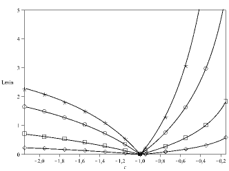
Figure 2: Comparison between the estimation for the position of the energy minimum of Eq. (22) (solid lines) and the values of $L_{min}$ obtained on the basis of the direct resolution of the Poisson-Boltzmann model (points). We chose $\sigma_{0}=-0.05\,e/$nm². Lengths are given in nm, and as functions of the ratio $r=\sigma_{L}/\sigma_{0}$, for different salt concentrations: $0.001$ M (asterisks), 0.01 M (circles), 0.1 M (squares), 1 M (diamonds).

In Fig. 2 we compare the previous expression Eq. (22) for $L_{min}$ with the corresponding values directly obtained from the numerical solution of the PB equation, for different salt concentrations and charge density ratios. The minimum positions $L_{min}$ are numerically estimated directly from the energy profiles. As expected, the formula of Eq. (22) exactly agrees with the numerical results.

Two limiting regimes can now be considered. Let introduce the Gouy-Chapman lengths for both plates, $\lambda_{0}=|1/2\pi\ell_{B}\sigma_{0}|$ and $\lambda_{L}=|1/2\pi\ell_{B}\sigma_{L}|$. In low salt conditions, $\lambda_{D}\gg\lambda_{0}$ and $\lambda_{D}\gg\lambda_{L}$. As a consequence, the position of the energy minimum is approximately given by

$$L_{min}\simeq 2\lambda_{D}\Big{|}\frac{1}{|{\sigma^{\prime}}_{L}|}-\frac{1}{|{\sigma^{\prime}}_{0}|}\Big{|}=|\lambda_{L}-\lambda_{0}|\;\;\;\;{\rm(low\;\;\;salt),}$$ (23)

In this limit, $L_{min}$ becomes therefore independent of the salt concentration and is only a function of the plates charge densities, i.e. of the ratio $r$ for the cases considered here since $\lambda_{0}$ is always kept fixed. In Fig. 3, we report the local ion distribution in the inter-plate space as a function of $x/L$ for a given choice of the plate charges and for different bulk ion concentrations $n_{b}$. At low salt (Fig. 3 a), the concentration of the counter-ions of the most charged plate is much larger than the salt concentration. In this case, the short range repulsion is therefore mainly due to the counter-ions of the most charged plate. We stress that the solid and dotted curves in Figure 2 also correspond to this low salt regime.

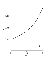
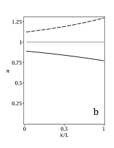
Figure 3: Positive (solid line) and negative (dashed line) ion distributions in the inter-plate space, at the equilibrium distance $L=L_{min}$, for the case of two charged plates with charge densities $\sigma_{0}=-0.05\,e/$nm² and $\sigma_{L}=0.1\,e/$nm², and for two different salt concentrations $n_{b}$: 0.001 M (low salt, a) and 1 M (high salt, b). The thick grey line indicates the value of the bulk ion concentration $n_{b}$.

Inversely, at high salt, $\lambda_{D}\ll\lambda_{0}$ and $\lambda_{D}\ll\lambda_{L}$, and the equilibrium is

$$L_{min}\simeq\lambda_{D}\;\;\Big{|}\ln{|\frac{{\sigma^{\prime}}_{0}}{{\sigma^{\prime}}_{L}}|}\Big{|}=\lambda_{D}\;\;\Big{|}\ln{|\frac{{\sigma}_{0}}{{\sigma}_{L}}|}\Big{|}\;\;\;\;{\rm(high\;\;\;salt).}$$ (24)

In this limit the estimated equilibrium length $L_{min}$ is then proportional to the Debye length, i.e. to $n_{b}^{-1/2}$. As shown in Fig. 3 b, the short range repulsion is indeed essentially due to the salt ions whose osmotic effect is modulated by the charges on the plates. The dashed and dot-dashed curves in Figure 2 correspond to the high salt regime. In this high salt regime, a good approximated expression for the equilibrium position can also be obtained in the framework of the linearised PB equation, as expected. We checked indeed that the resulting expression Parsegian matches well the curves in Fig. 2 for any ratios $r$ at high salt concentrations (data not shown). Instead, the linear PB approximation cannot reproduce the observed behavior at low salt, whereas the expression of Eq. (22) remains exact.

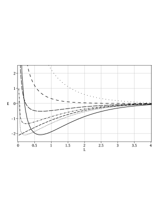
Figure 4: The interaction energy per unit surface $E$ ($k_{B}T/$100 nm²) for the interaction of a plate of charge density $\sigma_{0}=-0.05\,e/$nm² at $x=0$ with different plates of charge densities $\sigma_{L}$, as a function of the distance $L$ (nm) between them. The ratio $r=\sigma_{L}/\sigma_{0}$ between the densities varies from $-2$ to $1$ according to the figure legend. The plates are immersed in a 0.1 M monovalent solution.

How the $P=0$ condition should be interpreted in terms of electrostatic and osmotic contributions? The mechanism leading to an equilibrium position is not difficult to understand, starting from the expression of the excess pressure, Eq. (21). As already observed, the pressure is proportional to the constant of motion $C$ and is therefore constant in the inter-plate space $x\in[0,L]$. Let then consider the pressure $P$ exerted on one plate, e.g. at $x=0$. In this limit, the electrostatic term in Eq. (21) simply reads $-{k_{B}T}\;\sigma_{0}^{2}\;/2$, and is therefore independent of $L$. On the contrary, the osmotic term depends on the ion concentration and is therefore a function of $L$. We then note that the expression for the ion density, Eq. (7) can be rewritten in terms of the bulk concentrations and of the reduced potential as

$$\overline{n}_{\alpha}(x)={n}_{b}e^{-z_{\alpha}\overline{\psi}(x)}\,.$$ (25)

The equilibrium condition $P=0$, when calculated both on the left and right plates, can thus be written as a condition for the mean field potential at the boundaries that reads

$$\cosh{\overline{\psi}_{0}(L_{eq})}=\frac{\pi\ell_{B}\sigma_{0}^{2}}{n_{b}}+1\,.$$ (26)

$$\cosh{\overline{\psi}_{L}(L_{eq})}=\frac{\pi\ell_{B}\sigma_{L}^{2}}{n_{b}}+1\,.$$ (27)

where we introduced $\overline{\psi}_{0}(L)=\overline{\psi}(x=0)$ and $\overline{\psi}_{L}(L)=\overline{\psi}(x=L)\;\;\forall\>L\>\in\>\>[0,\infty[$, and where $L_{eq}$ is a distance between the plates for which $P=0$.

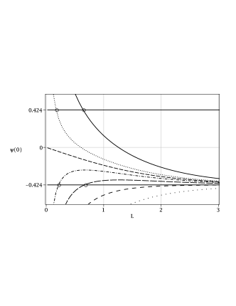
Figure 5: The adimensional mean field potential at $x=0$, $\overline{\psi}(0)$, as a function of the inter-plate distance $L$ (nm) and for the same ionic strength and charge density ratios of Fig. 4. The two horizontal lines correspond to the two roots $\pm$ arccosh${\left(\pi\ell_{B}\sigma_{0}^{2}/{n}_{b}\,+\,1\right)}$ of the left plate equilibrium condition, Eq. (26). The circles emphasize the non trivial solutions leading to an equilibrium position.

From now on we will focus on the case of asymmetrically and oppositely charged plates, $r<0$. In Figure 5 we compare the adimensional potential $\overline{\psi}_{0}(L)$ to the two roots $\pm$arccosh${\left(\pi\ell_{B}\sigma_{0}^{2}/{n}_{b}\,+\,1\right)}$ of Eq. (26). A trivial solution to Eqs. (26) and (27) corresponds to the limit $L\rightarrow\infty$, where $P=0$ by construction. In this limit, and typically for $L\gg\lambda_{0}+\lambda_{L}$, each plate charge is neutralized by its cloud of counterions as if the other plate didn’t exist. At a large enough distance $x$ from the plates, therefore, the ionic atmosphere behaves as an ideal gas and its pressure contribution $\Pi(x)$ exactly compensates the reservoir pressure $\Pi_{\infty}$. We also note that, in this case, according to (25), the sign of $\overline{\psi}_{0}$ and $\overline{\psi}_{L}$ at infinity are opposite for oppositely charged plates.

Let now look for another, finite solution of Eqs. (26) and (27) leading to $L_{eq}=L_{min}$. For this case, we only have to determine the sign of $\overline{\psi}_{0}(L_{min})$ and $\overline{\psi}_{L}(L_{min})$. It easy to see that the only possible solution is that the counterions of one plate prevail on both plates, so that the signs are both equal. It is the potential of the less charged plate that will change its sign at a given distance $L$ between infinity and $L_{min}$. In Figure  5 we show indeed that the sign of the adimensional potential $\overline{\psi}_{0}$ changes for $r<-1$ whereas it remains the same when $r>-1$. The opposite arises for $\overline{\psi}_{L}$ (data not shown).

The physical interpretation of the observed equilibrium is thus straightforward. The most charged plate carries its cloud of condensed counterions when approaching the less charged one. The counterions of the less charged plate are more easily released in the bulk when the two ion clouds overlap. This process continues until the electroneutrality constraint precludes a further release of ions, this leading the ion concentration, and therefore the repulsive osmotic pressure, to increase. The equilibrium is then obtained at the distance $L_{min}$ where electrostatic attraction and osmotic repulsion exactly balance.

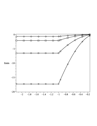
Figure 6: Comparison between the estimation of the energy minimum of Eq. (28) (solid lines) and the values of the energy at the minimum position $L_{min}$ obtained by direct integration of the Poisson-Boltzmann model, for different salt concentrations: $0.001$ M (asterisks), 0.01 M (circles), 0.1 M (squares), 1 M (diamonds). We have udes again $\sigma_{0}=-0.05\,e/$nm². In order to use more natural units, energies are given in units of $k_{B}T/$ 100 nm².

IV.2 Energy value $E_{min}$ at the minimum

We have shown that the pressure always vanishes at a given inter-plate distance for oppositely, asymmetric charged plates. Nevertheless, if the presence of a vanishing pressure always corresponds in principle to an equilibrium position between the plates, it does not guarantee by itself that this equilibrium position will be stable enough to be relevant from a thermodynamic point of view. Indeed, in order to assess the real existence of a stable equilibrium, we need to estimate the corresponding energy gain. We stress again that, if the energy gain at the minimum is small with respect to $k_{B}T$, the two charged bodies will behave as in the absence of electrostatic interaction (the energy going to zero at large distances). On the contrary, a deep minimum will make the bodies stabilize at a non-zero equilibrium distance.

The explicit calculation of the whole function $P(L)$ allows us to evaluate the energy profile $E(L)$ and compare the depth of the potential well to the thermal energy $k_{B}T$. The energies per unit area are shown in Fig. 4 (bottom), for the same charge densities as considered above. In order to use more natural units, energies are given in units of $k_{B}T/$ 100 nm². As expected, an energy minimum always exists for $r<0$ and $r\neq-1$. Interestingly, while for $0<r<1$ the energy minimum depth shows a relevant dependence on the second plate charge density $\sigma_{L}$, this dependence disappears for $r<-1$ where the depth becomes constant.

A more systematic investigation of the energy minimum depth for varying charge densities and salt conditions is shown in Figure 6. The value of the energy per a unit area of 100 nm² for different ionic strengths is given as a function of the ratio of the plates charge densities $r$, again for $\sigma_{0}$ fixed at $-0.05\,e/$nm². In low salt, the energy minimum depends on the ratio $r$ and on the salt concentration, and it reaches its maximum value for $r=-1$, i.e. when the position of the minimum degenerates to $L=0$. Energy depths are up to roughly $10$ $k_{B}T$ per 100 nm². Figure 6 also confirms that the minimum depth becomes constant for $r<-1$, and coincides in this case with its (maximum) value at the singular value $r=-1$.

In his paper, Ohshima Ohs75 also obtains an analytic expression for the energy at the minimum. An equivalent calculation, adapted to our formalism, is presented in Appendix B. The final result reads

$$\beta E_{min}=8n_{b}\lambda_{D}\;\left\{\sqrt{|{\sigma^{\prime}}_{m}|^{2}+4}-2-|{\sigma^{\prime}}_{m}|\;\mathrm{arcsinh}|\frac{{\sigma^{\prime}}_{m}}{2}|\right\}\,,$$ (28)

where ${\sigma^{\prime}}_{m}$ is the adimensional charge parameter related to the smallest plate charge density, i.e. ${\sigma^{\prime}_{m}}=\min{({\sigma^{\prime}_{0}},{\sigma^{\prime}_{L}})}$. In Figure 6 we compare the previous expression for the value of the energy depth with the results obtained by direct integration of the Poisson-Boltzmann equation. The two results show a perfect agreement. Together with Equation (22), the last result allows to a rapid and precise estimate of the equilibrium position and strength, and represent therefore a powerful tool in order to study the effective interaction between charged bodies in solution.

Figure 7: Sketch for the calculation of the interacting area for the case of two identical spheres. The area of each dashed spherical surface is $S=\frac{\pi}{4}(d^{2}+4h^{2})$.

Nevertheless, we have to stress finally that Equation (28), as well as Figures 4 and 6, only give the energy per unit area (fixed to 100 nm² in the Figures). To obtain the total energy between two charged bodies in solution and compare it to the thermal energy, the surface and geometry of the bodies should be taken into account. This roughly amounts to multiply the energy by an effective interaction area, but the estimation of this area is not easy in that it depends on the bodies shape. Indeed, the variation of the interaction with the distance should be included in the calculation of the effective interaction area. A typical choice is the use of the Derjaguin approximation Der34 ; Whi83 , that calculates the interaction energy $U$ between two curved surfaces by integrating the interaction energy per unit area between two flat plates $E(L)$ as

$$U\simeq\int_{A}E(L)dA\simeq f([R_{1}],[R_{2}])\int_{D_{min}}^{\infty}E(L)dL\,,$$ (29)

where $D_{min}$ is the distance of closest approach between the two curved surfaces, $dA$ is the differential area of the surfaces facing each other, $[R_{1}]$ and $[R_{2}]$ represent the sets of principal radii of curvature of the surfaces 1 and 2, respectively, at the distance of closest approach, and $f([a1],[a2])$ is a function of the radii of curvature of the surfaces. A very rough estimate should consider that the interaction between the two surfaces becomes negligible when their distance becomes larger than the screening Debye length $\lambda_{D}$. In a $0.1$ M solution, the Debye length is of the order of 1 nm. For the case of two spherical colloids of 100 nm diameter, (it varies from approximately 0.3 nm for an 1 M solution to 10 nm for 0.01 M). If the two spheres are in contact (i.e. for $L=0$), a simple geometric construction (depicted schematically in Fig. 7) allows to calculate the surface area on each sphere that is separate by less than a Debye length from the facing one, this leading to a surface of the order of 300 nm² (roughly 1 % of the whole sphere surface). As a consequence, the depth of the energy well would reach approximately $\sim$20 $k_{B}T$ in these conditions, and be thus large enough to ensure its stability at ordinary thermal conditions. Note however, that the two spheres will not be in contact anymore at equilibrium, but at a distance close to $L_{min}$, which can vary from $0$ to approximately $2$ nm depending on the value of the ratio $r$. When this distance becomes comparable to $\lambda_{D}$, the interaction area decreases considerably. Therefore, the actual interaction surface will be in general reduced to a value that depends on the two lengths $L_{min}$ and $\lambda_{D}$, and should be calculated case by case. Note that, in this sense, the shape of the two interacting bodies is bound to play a crucial role, in that it can modify considerably the distances between the facing surfaces and consequently the effective interaction area.

V Summary and conclusion

In this paper we derived, within the genuine framework of the Poisson-Boltzmann approximation, the main quantities of interest for the interaction between two charged surfaces in solution.

Interestingly, such a rigorous derivation brings up an extended formula for the interplate pressure, formally differing from the usual expression (giving the sum of electrostatic and osmotic contributions) by an extra-term. While in the considered case of fixed charges boundary conditions, this additional term vanishes and we recover the standard expression for the pressure, the question arises whether it leads to a modified result when different boundary conditions are considered. We recalled that the Poisson-Boltzmann free energy is properly used as the reference thermodynamic potential only at fixed charges. To show how the choice of the thermodynamic potential depends on the boundary conditions, we explicitely solved the problem in the fixed potential case, and show how to recover the physical meaningful pressure in that case. These precisions on the interplay between boundary conditions and thermodynamic ensemble have been obtained here thanks to a detailed and deductive derivation from the very basis of the Poisson-Boltzmann approach. Let us stress once again that shortcutting the details of the mathematical derivation potentially leads to underappreciate the role of the boundary conditions.

We then explicitely solved the problem in the simple case of a 1:1 salt solution and observed a very rich behavior as a function of the ratio of the plates charge densities and of the salt concentration, with a non trivial equilibrium position arising in large intervals of these parameters. The distance at which the osmotic and electrostatic pressures are in equilibrium is finely tuned by the system parameters. Such equilibrium position can stabilize two asymmetrically charged bodies at a nonzero distance, provided that the corresponding free energy gain is large enough compared to the thermal noise. At a given temperature, the stability of the complex can therefore be assessed only by explicitly calculating the depth of the corresponding energy well. We obtained a readily available answer to this problem by deriving analytic expressions for the position and depth of the energy well, by a reactualized version of the overlooked derivation of Ohshima Ohs75 .

In order to compare the energy values with the thermal energy, an estimation of the interaction area is also necessary. As an example, we gave an estimation for the typical case of spherical colloids, and found that the interaction energy well is typically of the order of several $k_{B}T$, this leading to a quite deep minimum. This estimation is only a rough approximation because, for a given problem either in biological or colloidal systems, the behavior of the two interacting bodies is strongly dependent not only on salt conditions and on the bodies charge but also on their shape. The relevance of the minimum is consequently rather delicate to compute and model-dependent.

APPENDICES

A Determination of the minimum position.

Starting from Eq. (12) and taking into account the contribution of the surrounding ions as in Eq. (21), one can obtain a suitable form for the excess free energy that will allow one to evaluate its amplitude at a given position $x$. We start by writing the excess free energy as

$$\beta\mathcal{F}_{PB}[\sigma,\{\overline{n}\}] = \int_{0}^{L}\left[\frac{1}{8\pi\ell_{B}}\left(\frac{d\overline{\psi}}{dx}\right)^{2}-\sum_{\alpha=1}^{2}\overline{n}_{\alpha}(x)\right]\;dx$$ (A1)

$$+\,2n_{b}\,L\,+\,\sum_{\alpha=1}^{2}\int_{0}^{L}\overline{n}_{\alpha}[-z_{\alpha}\overline{\psi}(x)]\;dx$$

where the $2n_{b}\,L$ term arises from the $\Pi_{\infty}$ contribution. Now, using (11) and (9) one finds:

$$\beta\mathcal{F}_{PB}[\sigma\{\overline{n}\}] = 2n_{b}\left\{\left(\frac{1}{2}C^{\prime}+1\right)L+\int_{0}^{L}\overline{\psi}(x)\sinh\overline{\psi}(x)\;dx\right\}$$ (A2)

$$= 2n_{b}\left\{\left(\frac{1}{2}C^{\prime}+1\right)L+\lambda_{D}^{2}\left[\overline{\psi}(x)\frac{d\overline{\psi}}{dx}\right]_{0}^{L}\right.$$

$$\hskip 56.9055pt-\left.\lambda_{D}^{2}\int_{0}^{L}\left(\frac{d\overline{\psi}}{dx}\right)^{2}dx\right\}$$

where we have introduced the Debye length, $\lambda_{D}=1/\sqrt{8\pi\ell_{B}\;n_{b}}$, $C^{\prime}=C/(4\pi\ell_{B}n_{b})$ and we performed an integration by part for the last equation.

In order to calculate $L_{min}$, it is convenient to introduce the following adimensional parameters:

$$\eta=x/\lambda_{D}$$ (A3)

$$\gamma(\eta)=\overline{\psi}(x)$$ (A4)

$$\theta(\eta)=\frac{d\gamma}{d\eta}\,.$$ (A5)

In terms of these variables, the Poisson-Boltzmann equation just writes

$$\frac{d\theta}{d\eta}=\sinh\gamma$$ (A6)

with the boundary conditions

$$\theta(0)=-{\sigma^{\prime}}_{0}=-4\pi\ell_{B}\lambda_{D}\sigma_{0}$$

$$\theta(\eta_{L})={\sigma^{\prime}}_{L}\;=\;\;\;4\pi\ell_{B}\lambda_{D}\sigma_{L}$$ (A7)

and the equivalent of Eq. (11), giving the constant of motion for the system, reads $\theta^{2}=2\cosh\gamma+C^{\prime}$. From this equation one gets

$$\frac{(\theta^{2}-C^{\prime})^{2}}{4}=\cosh^{2}\gamma=1+\sinh^{2}\gamma$$ (A8)

$$\frac{(\theta^{2}-C^{\prime})^{2}}{4}-1=\left(\frac{d\theta}{d\eta}\right)^{2}$$

$$\Rightarrow \left|\frac{d\eta}{d\theta}\right|=\frac{1}{\sqrt{(\theta^{2}-C^{\prime})^{2}/4-1}}$$

By integrating $\eta$ from $0$ to $\eta_{L}$, with $\left|d\eta\right|=d\eta$, we thus obtain

$$\int_{\theta(0)}^{\theta(\eta_{L})}\left|\frac{d\eta}{d\theta}\right|\;d\theta=\int_{0}^{\eta_{L}}d\eta\frac{d\theta}{|d\theta|}\,.$$

We are interested here in the case of oppositely charged plates, where the energy minimum does exist. We have therefore to consider different cases. Let assume for the moment that $|{\sigma^{\prime}}_{0}|>|{\sigma^{\prime}}_{L}|$. If now ${\sigma^{\prime}}_{0}<0$ and ${\sigma^{\prime}}_{L}>0$, then $\theta(0)$ and $\theta(\eta_{L})$ have both positive values and $|d\theta|=-d\theta$. We then have

$$\eta_{L}=\int_{|{\sigma^{\prime}}_{L}|}^{|{\sigma^{\prime}}_{0}|}\left|\frac{d\eta}{d\theta}\right|\;d\theta\hskip 28.45274pt{\sigma^{\prime}}_{0}<0,\;\;{\sigma^{\prime}}_{L}>0\,.$$ (A9)

On the other hand, if ${\sigma^{\prime}}_{0}>0$ and ${\sigma^{\prime}}_{L}<0$, then $\theta(0)$ and $\theta(\eta_{L})$ have both negative values and $|d\theta|=d\theta$. We thus obtain

$$\eta_{L}=-\int_{-|{\sigma^{\prime}}_{L}|}^{-|{\sigma^{\prime}}_{0}|}\left|\frac{d\eta}{d\theta}\right|\;d\theta\hskip 28.45274pt{\sigma^{\prime}}_{0}>0,\;\;{\sigma^{\prime}}_{L}<0\,.$$ (A10)

Nevertheless, since $\left|\ d\eta/d\theta\right|$ is only a function of $\theta^{2}$ we can make the change of variable $\Theta=-\theta$ in Eq.(A10) and retrieve the result (A9). Therefore, we always have

$$\eta_{L}=\int_{|{\sigma^{\prime}}_{L}|}^{|{\sigma^{\prime}}_{0}|}\frac{2}{\sqrt{(\theta^{2}-C^{\prime}+2)(\theta^{2}-C^{\prime}-2)}}\;d\theta$$ (A11)

If now $L={L_{min}}$, then $P=0$, i.e. $\Pi=\Pi_{\infty}=2k_{B}Tn_{b}$, and therefore $C^{\prime}=-2$. At the equilibrium position, Eq.(A11) becomes then

$$\eta_{L_{min}}=\int_{|{\sigma^{\prime}}_{L}|}^{|{\sigma^{\prime}}_{0}|}\frac{2}{\theta\sqrt{\theta^{2}+4}}\;d\theta=\int_{|{\sigma^{\prime}}_{L}|/2}^{|{\sigma^{\prime}}_{0}|/2}\frac{1}{\alpha\sqrt{\alpha^{2}+1}}d\theta$$

where we introduced $\alpha=\theta/2$. As a primitive function of $1/(x\sqrt{x^{2}+1})$ is $\ln\left(x/(1+\sqrt{x^{2}+1})\right)$, we get for the case $|{\sigma^{\prime}}_{0}|>|{\sigma^{\prime}}_{L}|$

$$\eta_{L_{min}}=\ln\left(\frac{|{\sigma^{\prime}}_{0}|(2+\sqrt{|{\sigma^{\prime}}_{L}|^{2}+4})}{|{\sigma^{\prime}}_{L}|(2+\sqrt{|{\sigma^{\prime}}_{0}|^{2}+4})}\right)\,.$$ (A12)

The extension to the opposite case of $|{\sigma^{\prime}}_{0}|<|{\sigma^{\prime}}_{L}|$ is straightforward, this leading to the following final formula for the position of the energy minimum $L_{min}=\lambda_{D}\eta_{L_{min}}$:

$$L_{min}=\lambda_{D}\Big{|}\ln{\Big{(}\frac{|\sigma^{\prime}_{0}|(2+\sqrt{{\sigma^{\prime}_{L}}^{2}+4})}{|\sigma^{\prime}_{L}|(2+\sqrt{{\sigma^{\prime}_{0}}^{2}+4})}\Big{)}}\Big{|}\,.$$

B Determination of the energy value at the minimum.

Following the main lines of the calculation presented in Ohs75 , we here look for an analytic expression for the energy at the minimum. In our framework, the interaction energy computed numerically directly from the integration of the excess pressure writes formally (by definition of the integration):

$$\beta E(L)=\beta(\mathcal{F}(L)-\mathcal{F}(\infty))$$ (B1)

where $\mathcal{F}(L)$ is given by (A2). By using the dimensionless parameters defined in the previous section, we have

$$\beta\mathcal{F} = \left\{(K(L)+J(L)-I(L)\right\}2n_{b}\lambda_{D}\,,$$ (B2)

with

$$K(L) = (\frac{1}{2}C^{\prime}+1)\eta_{L}\,,$$

$$J(L) = \Big{[}\gamma(\eta)\theta(\eta)\Big{]}_{0}^{\eta_{L}}\,,$$

$$I(L) = \int_{0}^{\eta_{L}}\theta^{2}\;d\eta\,.$$

We will now, first, calculate the three contributions to $\mathcal{F}(L_{min})$, and then the corresponding contributions to $\mathcal{F}(\infty)$.

Let start by calculating $I(L_{min})$. From the definition, we have

$$I(L_{min}) = \int_{0}^{\eta_{L_{min}}}\theta^{2}\left(\frac{d\eta}{d\theta}d\theta\right)=-\int_{|{\sigma^{\prime}}_{0}|}^{|{\sigma^{\prime}}_{L}|}\theta^{2}\left|\frac{d\eta}{d\theta}\right|d\theta$$ (B3)

$$= \int_{|{\sigma^{\prime}}_{L}|}^{|{\sigma^{\prime}}_{0}|}\frac{2\theta}{\theta^{2}+4}d\theta$$

$$= 2(\sqrt{|{\sigma^{\prime}}_{0}|^{2}+4}-\sqrt{|{\sigma^{\prime}}_{L}|^{2}+4})$$

where we used the fact that, on the $[0,\eta_{L}]$ range, $d\eta/d\theta=-|d\eta/d\theta|$.

To calculate $J(L_{min})$ we recall that when $L=L_{min}$ we have $\cosh\gamma(0)={{\sigma^{\prime}}}_{0}^{2}/2+1$. By using the relation $(\cosh x-1)/2=\sinh^{2}({x}/{2})$, we then get $\sinh^{2}\gamma(0)/2={{\sigma^{\prime}}}_{0}^{2}/4$, and thus

$$|\sinh\frac{\gamma(0)}{2}|=\frac{1}{2}|{{\sigma^{\prime}}}_{0}|$$ (B4)

In the same way we have

$$|\sinh\frac{\gamma(\eta_{L_{min}})}{2}|=\frac{1}{2}|{\sigma^{\prime}}_{L}|\,.$$ (B5)

We can now easily calculate $J(L_{min})$ starting from

$$J(L_{min}) = \gamma(\eta_{L_{min}})\,\theta(\eta_{L_{min}})-\gamma(0)\,\theta(0)$$

$$= \gamma(\eta_{L_{min}})\,|{\sigma^{\prime}}_{L}|+\gamma(0)\,{\sigma^{\prime}}_{0}\,.$$

Now, at $L_{min}$, $\gamma(\eta_{L_{min}})$ and $\gamma(0)$ have the same sign, which is governed by the most charged plate. Let again focus on the case where ${\sigma^{\prime}}_{0}<0$ and $|{\sigma^{\prime}}_{0}|>|{\sigma^{\prime}}_{L}|$, as used in our illustrations. In this case, the sign of $\gamma(\eta_{L_{min}})$ and $\gamma(0)$ is the same as the sign of ${\sigma^{\prime}}_{0}$ (cf. Figure 4), this leading to

$$J(L_{min})=-2\,|{\sigma^{\prime}}_{L}|\;\mathrm{arcsinh}|\frac{{\sigma^{\prime}}_{L}}{2}|-2\,|{\sigma^{\prime}}_{0}|\;\mathrm{arcsinh}|\frac{{\sigma^{\prime}}_{0}}{2}|$$ (B6)

We easily obtain that $K(L_{min})=0$ since $C^{\prime}=-2$ for $L=L_{min}$.

The overall result for $\mathcal{F}(L_{min})$ reads therefore

$$\beta\mathcal{F}(L_{min})=4n_{b}\lambda_{D}\;\left\{-|{\sigma^{\prime}}_{L}|\;\mathrm{arcsinh}|\frac{{\sigma^{\prime}}_{L}}{2}|\right.$$ (B7)

$$-|{\sigma^{\prime}}_{0}|\;\mathrm{arcsinh}|\frac{{\sigma^{\prime}}_{0}}{2}|\left.-(\sqrt{|{\sigma^{\prime}}_{0}|^{2}+4}-\sqrt{|{\sigma^{\prime}}_{L}|^{2}+4}\,)\right\}\,.\hskip 22.76219pt$$

Let now calculate $\mathcal{F}(\infty)$. We have to be quite cautious to compute $I(\infty)$. Indeed, we have

$$I(\infty)=\lim_{\eta_{L}\rightarrow\infty}\int_{0}^{\eta_{L}}\theta^{2}\left(\frac{d\eta}{d\theta}d\theta\right)\,,$$

and the point is that $d\eta/d\theta$ has not the same sign all over the range $[0,\infty[$. Actually because of the infinite distance between the two plates, each plate tends to behave as a single plate in this limit, and thus there exists a distance for which $\theta=0$. So, $\theta$ will be initially equal to $|{\sigma^{\prime}}_{0}|$, then decrease to zero and increase again to $|{\sigma^{\prime}}_{L}|$. We have therefore:

$$I(\infty) = -\int_{|{\sigma^{\prime}}_{0}|}^{0}\theta^{2}\left|\frac{d\eta}{d\theta}\right|\,d\theta+\int_{0}^{|{\sigma^{\prime}}_{L}|}\theta^{2}\left|\frac{d\eta}{d\theta}\right|\,d\theta$$ (B8)

$$= -\left[2\sqrt{\theta^{2}+4}\right]_{|{\sigma^{\prime}}_{0}|}^{0}+\left[2\sqrt{\theta^{2}+4}\right]^{|{\sigma^{\prime}}_{L}|}_{0}$$

$$= -8+2\sqrt{|{\sigma^{\prime}}_{0}|^{2}+4}+2\sqrt{|{\sigma^{\prime}}_{L}|^{2}+4}\,.$$

Besides, we have for $J(\infty)$:

$$J(\infty) = \gamma(\infty)|{\sigma^{\prime}}_{L}|-\gamma(0)|{\sigma^{\prime}}_{0}|$$

$$= 2\,|{\sigma^{\prime}}_{L}|\;\mathrm{arcsinh}|\frac{{\sigma^{\prime}}_{L}}{2}|-2\,|{\sigma^{\prime}}_{0}|\;\mathrm{arcsinh}|\frac{{\sigma^{\prime}}_{0}}{2}|$$

because it’s only the reduced potential $\gamma$ corresponding to the plate with the lowest charge (in absolute value) that changes its sign between $L_{min}$ and $L_{\infty}$ (cf. again Figure 4).

When there is an infinite distance between the plates we also have $C^{\prime}=-2$ (intuitively because there is no more interaction between the plates) and thus $K(\infty)=0$. We then have:

$$\beta\mathcal{F}(\infty)=4n_{b}\lambda_{D}\;\left\{|{\sigma^{\prime}}_{L}|\mathrm{arcsinh}|\frac{{\sigma^{\prime}}_{L}}{2}|\right.$$ (B10)

$$-|{\sigma^{\prime}}_{0}|\mathrm{arcsinh}|\frac{{\sigma^{\prime}}_{0}}{2}|\left.-(-4+\sqrt{|{\sigma^{\prime}}_{0}|^{2}+4}+\sqrt{|{\sigma^{\prime}}_{L}|^{2}+4})\right\}\,.$$

From the evaluation of Equation (B1) at $L=L_{min}$, we get then finally the following expression for the energy at the minimum in the case when ${\sigma^{\prime}}_{0}<0$ and $|{\sigma^{\prime}}_{0}|>|{\sigma^{\prime}}_{L}|$:

$$\beta E_{min}=8n_{b}\lambda_{D}\;\left\{\sqrt{|{\sigma^{\prime}}_{L}|^{2}+4}-2-|{\sigma^{\prime}}_{L}|\;\mathrm{arcsinh}|\frac{{\sigma^{\prime}}_{L}}{2}|\right\}\,.$$ (B11)

On the other hand, one can easily be convinced that inverting the roles of $|{\sigma^{\prime}}_{0}|$ and $|{\sigma^{\prime}}_{L}|$ leads to the same expression as Eq. (B11) where $|{\sigma^{\prime}}_{0}|$ and $|{\sigma^{\prime}}_{L}|$ are inverted. Therefore, the very general result writes (Eq. (28))

$$\beta E_{min}=8n_{b}\lambda_{D}\;\left\{\sqrt{|{\sigma^{\prime}}_{m}|^{2}+4}-2-|{\sigma^{\prime}}_{m}|\;\mathrm{arcsinh}|\frac{{\sigma^{\prime}}_{m}}{2}|\right\}\,,$$

where ${\sigma^{\prime}}_{m}$ is related to the smallest plate charge density, i.e. ${|\sigma^{\prime}_{m}|}=\min{({|\sigma^{\prime}_{0}|},{|\sigma^{\prime}_{L}|})}$.

References

- (1) Kung W. and Lau A. W. C. Charged plates beyond mean field: One loop corrections by salt density Fluctuations cond-mat/0603191 preprint (2006)
- (2) Borukhov I., Andelman D. and Orland H. Steric Effects in Electrolytes: A Modified Poisson-Boltzmann Equation Phys. Rev. Lett. 79 435 (1997)
- (3) Borukhov I., Andelman D. and Orland H. Adsorption of Large Ions from an Electrolyte Solution: A Modified Poisson-Boltzmann Equation Electrochimica Acta 46 221 (2000)
- (4) Netz R. R, and Orland H. Beyond Poisson Boltzmann: Fluctuations effects and correlation functions Eur. Phys. J. E, 1, 203-214 (2000)
- (5) Deserno M. et al. Cell model and Poisson Boltzmann theory: a brief introduction in Proceedings of the NATO Advanced Study Institute on Electrostatic Effects in Soft Matter and Biophysics, edited by C. Holm, P. Kékicheff and R. Podgornik (Kluwer, Dordrecht, 2001)
- (6) Tang, C., Iwahara, J. and Clore, G. M. Visualization of transient encounter complexes in protein protein association Nature 444 383-386 (2006)
- (7) von Hippel, H. Diffusion driven mechanism of protein translocation on nucleic acids. III. The E. coli lac repressor-operator interaction: kinetic measurements and conclusions Biochemistry 20 6961-6977 (2007)
- (8) Sens P. and Joanny J.-F. Counterion Release and Electrostatic Adsorption Phys. Rev. Lett. 84 4862-4865 (2000)
- (9) Parsegian V. and Gingell D. On the electrostatic interaction across a salt solution between two bodies bearing unequal charges Biophys. J. 12 1192-1204 (1972)
- (10) Verwey E. J. W. and Overbeek J. TH. G. Theory of the stability of Lyophobic Colloids (Elsevier, Amsterdam, 1948)
- (11) Bhattacharjee S., Elimelech M.and Borkovec M. DLVO Interaction between Colloidal Particles: Beyond Derjaguin’s Approximation CROATICA CHEMICA ACTA CCACAA 71 883-903 (1998)
- (12) Bhattacharjee S. and Elimelech M. Surface Element Integration: A novel Technique for Evaluation of DLVO Interaction between a particle and a flat plate Journ. Coll. and Inter. Sci. 193, 273-285 (1997)
- (13) Tamashiro M. N. and Schiessel H. Where the linearized Poisson-Boltzmann cell model fails: the planar case as a prototype study Phys. Rev. E, 68, 066106 (2003)
- (14) Zypman F. R. Exact expressions for colloidal plane-particle interaction forces and energies with applications to atomic force microscopy J. Phys. Condens. Matter 18 2795-2803 (2006)
- (15) Lau A. W-C. Fluctuation and correlations effects in electrostatics of Highly-Charged Surfaces PhD Thesis (Oct. 2000)
- (16) Hansen J-P. and McDonald I. R. Theory of Simple Liquids (Academic Press, London, Third Edition, 2006)
- (17) Carnie S. L. and Torrie G. M. The Statistical Mechanics of the Electrical Double Layer Adv. Chem. Phy. 56 141 (1984)
- (18) Marcus R. A. Calculation of Thermodynamic Properties of Polyelectrolytes J. Chem. Phys. 23 1057 (1955)
- (19) Wennerström H., Jönsson B. and Linse P. The cell model for polyelectolyte systems J. Chem. Phys. 76 4665 (1982)
- (20) Lau A. and Pincus P. Binding of oppositely charged membranes and membrane reorganization Eur. Phys. J. B 10 175 (1999)
- (21) Ben-Yaakov D., Burak Y., Andelman D. and Safran S. A. Elecrostatic interactions of asymmetrically charged membranes Europhys. Lett., 79 48002 (2007)
- (22) Ohshima H. Diffuse double layer interaction between two parallel plates with constant surface charge density in an electrolyte solution III: Potential energy of double layer interaction Colloid and Polymer Sci. 253 150-157 (1975)
- (23) Huang K. Statistical Mechanics (Wiley, New-York, Second Edition, 1987)
- (24) Feynman R. P., Leighton R. B. and Sand M. The Feynman Lectures on Physics, Volume 2 (Addison-Wesley, Pearson PLC, 2006)
- (25) Trizac E. Electrostatically Swollen Lamellar Stacks and Adiabatic Pair Potential Charged Platelike Colloids in an Electrolyte Langmuir 17 4793-4798 (2001)
- (26) Bohinc K., Iglic, A. and May S. Interaction between macroions mediated by divalent rod-like ions Europhys. Lett. 68 494-500 (2004)
- (27) Derjaguin B. V. Untersuchungen uber die Reibung utid Adhusion Kolloid-Z. 69 155 (1934)
- (28) White L. R. On the Deryaguin approximation for the interaction of macrobodies J. Colloid Interface Sci. 95 286 (1983)