The NOAO NEWFIRM Pipeline
Abstract
The NOAO NEWFIRM Pipeline produces instrumentally calibrated data products and data quality measurements from all exposures taken with the NOAO Extremely Wide-Field Infrared Imager (NEWFIRM) at the KPNO Mayall 4-meter telescope. We describe the distributed nature of the NEWFIRM Pipeline, the calibration data that are applied, the data quality metadata that are derived, and the data products that are delivered by the NEWFIRM Pipeline.
Department of Astronomy, University of Maryland, MD, USA
National Optical Astronomy Observatory, Tucson, AZ, USA
1. Introduction
The NOAO Extremely Wide-Field Infrared Imager (NEWFIRM) is a 1 to 2.4 micron IR camera for both the Kitt Peak and CTIO 4m telescopes. The instrument is equipped with broad and narrow band filters. The focal plane of NEWFIRM consists of four 2048 by 2048 detectors laid out in a 2 by 2 mosaic. The field of view is 27.6’ by 27.6’ (including a 35” wide gap between the detectors). The pixel size is 0.4”.
The data taken with NEWFIRM are processed by the NOAO NEWFIRM pipeline. This pipeline consists of two distinct components. The first is the Quick Reduce Pipeline (QRP), which produces reduced data in near-real time at the telescope. The second component is the Science Pipeline (SP). It produces uniformly reduced, high-quality data at the end of an observing block. The products of the SP will be made available to the observer and through the NOAO archive.
Both QRP and SP apply all basic calibration steps, such as dark subtraction, flat fielding, and sky subtraction. WCS solutions are also determined for each exposure by matching stars against the 2MASS catalog (Skrutskie et al., 2006). The stars in common with 2MASS are also used to determine a first-order photometric calibration. The QRP, as its final data product, combines data for the same pointing to create deep dither stacks. The SP continues, and uses these first stacks to create object masks, which are then used to mask out objects in the individual exposures for an improved second-pass sky subtraction and deep dither stacks. In addition, the SP also deals with the persistence seen in the NIR detector, large-field mosaicked images, and data quality metrics for calibration and science data.
2. A Distributed Pipeline System
Both the QRP and the SP make use of the NOAO High-Performance Pipeline System (Scott et al. 2007). This system is designed to run on a cluster of computers, and it allows easy and efficient use of CPU resources in problems with inherent parallelism such as the processing of observations from mosaic cameras.
In the pipeline system, the data reduction process has been organized into a hierarchical structure of different individual pipelines. Each of these pipelines deals with one aspects of the reduction process e.g., constructing calibration data (such as darks, dome flats, or master sky flats), applying these calibration data, collecting the final data products, and controlling other pipelines. All of these pipelines, in turn, are subdivided into a set of modules, each of which carries out a small step of the data reduction process. These modules can be written in any language. Because the pipeline system uses IRAF, most modules are IRAF scripts.
All of the pipelines and associated modules can be configured to run on all available nodes (or any subset thereof), ensuring maximum use of available resources. Whenever a pipeline is to be started, a node selection algorithm is called to find the best node by considering issues such as load and minimizing network traffic. Distribution of the work across the nodes in the cluster also depends on the nature of the steps in the data reduction process, and processing may be distributed for example by detector or by multi-extension fits (MEF) files. An example of distribution by detector is the calculation of the master sky flats from a group of observations. In this case, the data from the 4 different NEWFIRM detectors are sent to 4 different nodes, each of which will process the data from one unique array. When applying calibration data to MEF files, however, it is more efficient to leave the individual arrays on the same node, because this significantly reduces transfer of data between nodes. In this case, the data are distributed across nodes by MEF files.
To make sure available resources are used efficiently, any node can run multiple instances of a pipeline. Thus, on a node with two CPUs, two instances of a pipeline that apply calibration data to science observations will run in parallel.
3. Calibration
Both the QRP and the SP apply the major calibrations to the raw data:
-
•
Apply a correction for the inherently nonlinear nature of the NIR detectors
-
•
Subtract the dark structure (from dark exposures)
-
•
Apply flat fields
-
•
Flag any bad and saturated pixels, and pixels affected by persistence)
-
•
Do a first-pass sky subtraction using sky images constructed from other images in the observing sequence (for sparse field data) or from an offset sky field (e.g., when observing large objects).
-
•
For object exposures, determine the world coordinate system and a rough photometric zeropoint by matching objects in the field against the 2MASS catalog
For the QRP, the emphasis is on speed of processing while still producing data that are reduced thoroughly and allow the users to evaluate the quality and depth of their data. The SP generates advanced data products by also including the following time-consuming steps:
-
•
2nd pass sky sky subtraction (masks are used to remove objects when exposures are combined to create sky images)
-
•
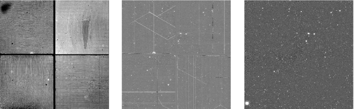
Detection and flagging of transient events (e.g., cosmic ray hits, satellite and airplane trails)
-
•
Object masking in offset-sky exposures for improved sky subtraction

4. Data Quality
The QRP and the SP verify, check, and characterize the data being processed throughout the reduction process, and the resulting metadata is stored. This is done for several reasons:
-
•
Immediately after ingesting the data, the fits files and headers are verified and data that cannot be processed are rejected. Examples are: corrupt or incomplete fits files, fits files with missing critical header keywords. When possible, missing keywords are reconstructed.
-
•
Statistics and other numerical characterizations of individual calibration exposures are compared against expected values and outliers are rejected.
-
•
Critical metrics that help users evaluate the quality of the data, such as seeing, photometric depth, sky level, and WCS are recorded. In the case of the QRP, these metrics are presented to the user both for the most recent data, and also for prior observations for trending purposes.
For the SP, a more exhaustive set of metrics is measured for calibration and science data. These metadata, derived from the raw data, intermediate steps, and the final pipeline data products are all stored in the pipeline metadata database. This database can be queried by the pipeline itself to carry information from one module to the next, but it also provides a means to investigate long term trends in the instrument’s performance.
5. Data products
After the exposures have been fully calibrated, the data are reprojected to the same orientation and pixel size, and to the closest tangent point on a predefined grid (thus ensuring that spatially close exposures have the same tangent point), these exposures are then combined into one stacked image, which could span a large field of view, go deep, or both. The original reduced image, the resampled one, and the stacked one are end products of the pipeline. In addition, the pipeline produces masks for each of these.
References
Scott, D., Pierfederici, F., Swaters, R. A., Thomas, B., & Valdes, F. G. 2007, Astronomical Data Analysis Software and Systems XVI, 376, 265
Skrutskie, M.F., et al. 2006, AJ, 131, 1163