Convergence and Tradeoff of Utility-Optimal CSMA

Abstract

It has been recently suggested that in wireless networks, CSMA-based distributed MAC algorithms could achieve optimal utility without any message passing. We present the first proof of convergence of such adaptive CSMA algorithms towards an arbitrarily tight approximation of utility-optimizing schedule. We also briefly discuss the tradeoff between optimality at equilibrium and short-term fairness practically achieved by such algorithms.

I Model and Algorithm

I-A Network model and optimization problem

Consider a wireless network composed by a set ${\cal L}$ of $L$ interfering links. Interference is modeled by a symmetric, boolean matrix $A\in\{0,1\}^{L\times L}$, where $A_{lk}=1$ link $l$ interferes link $k$. Define by ${\cal N}\subset\{0,1\}^{L}$ the set of feasible link activation profiles, or, schedules. A schedule $m\in{\cal N}$ is a subset of non-interfering active links. The transmitter of link $l$ can transmit at a fixed unit rate when active, and all links are saturated with infinite backlog.

Denote by ${\bm{\gamma}}=(\gamma_{l},l\in{\cal L})$ the long-term throughputs achieved by a scheduling algorithm, which determines which links are activated at each time. Let $U:\mathbb{R}^{+}\to\mathbb{R}$ be an increasing and strictly concave objective function. The following utility optimization problem over schedules has been extensively studied:

$$\max\quad \Sigma_{l\in{\cal L}}U(\gamma_{l}),\quad\hbox{s.t. }\forall l\in{\cal L},\gamma_{l}\leq\Sigma_{m:l\in m}\pi_{m}$$ (1)

$$\forall m\in{\cal N},\pi_{m}\geq 0,\Sigma_{m\in{\cal N}}\pi_{m}=1.$$

where $\pi_{m}$ is the long-term proportion of time when schedule $m$ is used. We denote by $\overline{{\bm{\gamma}}}=(\overline{\gamma}_{l},l\in{\cal L})$ the solution of (1). Most of the proposed distributed schemes to solve (1) make use of a dual decomposition of the problem into a rate control and a scheduling problem: A virtual queue is associated to each link; a rate control algorithm defines the rate at which packets are sent to the virtual queues, and a scheduling algorithm decides, depending on the level of the virtual queues, which schedule to use with the aim of stabilizing all virtual queues. The main challenge reduces to developing a distributed and efficient scheduling algorithm. Most of the proposed solutions are semi-distributed implementations of the max-weight scheduler introduced in [1], and require information about the queues to be passed around among the nodes or links (e.g., see a large set of references in [2]). This signaling overhead increases communication complexity and reduces effective throughput of the algorithms.

Recently, there have been proposals that do not use any message passing, and yet achieve high efficiency [3, 4, 5]. These algorithms are based on the random access protocol of CSMA (Carier Sense Multiple Access), and leverage simulated annealing techniques to solve the max-weight scheduling problem as first proposed in [6]. In this paper we provide the first rigorous proof that such adaptive CSMA algorithms indeed converge, using stochastic approximation tools with two time-scales. Then, we quantify the impact of inevitable collisions in CSMA protocols on the trade-off between their long-term efficiency and short-term fairness, the latter defined here as $\beta={1/\max\{E_{l},l\in{\cal L}\}}$, where $E_{l}$ is the average duration during which link $l$ do not transmit successfully. It turns out that a price to pay for the surprisingly good utility performance by these message-passing-free algorithms is short-term starvation.

I-B Adaptive CSMA algorithms

To access the channel, each transmitter $l\in\mathcal{L}$ runs a random back-off algorithm parametrized by two positive real numbers $(\lambda_{l},\mu_{l}),$ denoted as CSMA$(\lambda_{l},\mu_{l})$: after a successful transmission, the transmitter randomly picks a back-off counter according to some distribution of mean $\lambda_{l}$; it decrements the counter only when the channel is sensed idle; and it starts transmitting when the back-off reaches 0, and remains active for a duration $\mu_{l}$.

We first consider a continuous-time and then a discrete-time version of CSMA algorithms. In the ideal continuous-time setting (considered in this and the next sections), the back-off counter distribution is exponential, so that two interfering links cannot be activated simultaneously and collisions are avoided. In practice, back-offs are discrete, say geometrically distributed. In this discrete setting (studied in Section III), collisions may occur, degrade performance, and introduce tradeoff between long-term utility and short-term fairness.

If parameters $(\lambda_{l},\mu_{l}),l\in{\cal L}$ were fixed, the analysis of the dynamics of systems under continuous-time CSMA algorithms would be classical (e.g., [7] and references therein). In this case, in steady state the set of active links evolves according to a reversible Markov process whose stationary distribution, denoted by $\pi^{\bm{\lambda},\bm{\mu}}$, is defined by:

$$\forall m\in{\cal N},\pi^{\bm{\lambda},\bm{\mu}}(m)={\prod_{l\in m}\lambda_{l}\mu_{l}\over\sum_{m^{\prime}\in{\cal N}}\prod_{l\in m^{\prime}}\lambda_{l}\mu_{l}}.$$ (2)

We now describe how transmitters adapt their CSMA parameters. Time is slotted and transmitters update their parameters at the beginning of each slot. To do so, they maintain a virtual queue, denoted by $q_{l}[t]$ in slot $t$, for link $l$. The algorithm operates as follows (the algorithm presented here is an extension of those proposed in [3]):
Algorithm 1.

1. During slot $t$, the transmitter of link $l$ runs CSMA($\lambda_{l}[t],\mu$), and records the amount $S_{l}[t]$ of service received during this slot;

2. At the end of slot $t$, it updates its virtual queue and its CSMA parameters according to:

   $$q_{l}[t+1]=\bigg{[}q_{l}[t]+{b[t]\over W^{\prime}(q_{l}[t])}\big{(}U^{\prime-1}({W(q_{l}[t])\over V})-S_{l}[t]\big{)}\bigg{]}^{q^{\max}}_{q^{\min}},$$

   and set $\lambda_{l}[t+1]=\mu^{-1}\exp\{W(q_{l}[t+1])\}$.

At the beginning of each slot, each non-active transmitter picks a new random back-off counter to account for the CSMA parameter update. In Algorithm 1, $b:\mathbb{N}\to\mathbb{R}$ is a step size function; $W:\mathbb{R}^{+}\to\mathbb{R}^{+}$ is a strictly increasing and continuously differentiable function, termed weight function; $V$, $q^{\min}$, $q^{\max}(>q^{\min})$ are positive parameters, and $[\cdot]_{c}^{d}\equiv\max(d,\min(c,\cdot))$.

II Convergence Proof

The main difficulty in analyzing the convergence of Algorithm 1 lies in the fact that the updates in the virtual queues depend on random processes $(S_{l}[t],t\geq 0)$, whose transition rates in turn depend on the virtual queues. As we will demonstrate, it is possible to represent Algorithm 1 as a stochastic approximation algorithm with controlled Markov noise as introduced by Borkar [8].

We use the notation $\pi^{\bm{q}}$ to denote the distribution on ${\cal N}$ defined by:

$$\forall m\in{\cal N},\quad\pi^{\bm{q}}(m)={\exp(\sum_{l\in m}W(q_{l}))\over\sum_{m^{\prime}\in{\cal N}}\exp(\sum_{l\in m^{\prime}}W(q_{l}))}.$$ (3)

We also denote by $\bm{\gamma}[t]=(\gamma_{l}[t]={1\over t}\sum_{i=0}^{t-1}S_{l}[i],l\in{\cal L})$ the random variable representing the time-averaged service rates received by the various links over the interval $[0,t).$ The following theorem states the convergence of Algorithm 1, for diminishing step-sizes (similar but weaker results are readily obtained for constant, small step-sizes).

Theorem 1

Assume that $V\leq W(q^{\max})/U^{\prime}(1)$ and that $\sum_{t=0}^{\infty}b[t]=\infty,\quad\sum_{t=0}^{\infty}b[t]^{2}<\infty$. For any initial condition $\bm{q}[0]$, under Algorithm 1, we have the following convergence:

$$\lim_{t\to\infty}{\bm{q}}[t]=\bm{q}^{\star}\textrm{ and }\lim_{t\to\infty}\bm{\gamma}[t]=\bm{\gamma}^{\star},\textrm{ almost surely},$$

where $\bm{q}^{\star}$ and $\bm{\gamma}^{\star}$ are such that: $(\bm{\gamma}^{\star},\pi^{\bm{q}^{\star}})$ solves:

max $$V\Sigma_{l\in{\cal L}}U(\gamma_{l})-\Sigma_{m\in{\cal N}}\pi_{m}\log\pi_{m}$$ (4)

s.t. $$\gamma_{l}\leq\Sigma_{m\in{\cal N}:m_{l}=1}\pi_{m},\quad\Sigma_{m\in{\cal N}}\pi_{m}=1.$$ (5)

Furthermore, Algorithm 1 approximately solves (1) as:

$$\big{|}\Sigma_{l\in{\cal L}}\big{(}U(\overline{\gamma}_{l})-U(\gamma_{l}^{\star})\big{)}\big{|}\leq{\log|{\cal N}|/V}.$$ (6)

Proof. We first show that the network dynamics under the continuous-time random CSMA protocol can indeed be averaged and it asymptotically approaches to a deterministic trajectory (see Lemma 1). Resolving this bottleneck in understanding adaptive CSMA is the main contribution in this proof. Then we prove that the resulting averaged algorithm converges to the solution of (4).

Step 1. From the discrete-time sequence $(\bm{q}[t],t\geq 0)$, we define a continuous function $\bar{\bm{q}}(\cdot)$ as follows. Define for all $n$, $t_{n}=\sum_{i=1}^{n}b[i]$, and for all for all $t_{n}<t\leq t_{n+1}$,

$$\bar{q}_{l}(t)=q_{l}[n]+(q_{l}[n+1]-q_{l}[n])\times({t-t_{n}\over t_{n+1}-t_{n}}).$$ (7)

Lemma 1 (Convergence and averaging)

Denote by $\tilde{q}$ the solution of the following system of o.d.e.’s: for all $l$,

$${d\tilde{q}_{l}/dt}=\left(U^{\prime-1}\Big{(}{W_{l}(\tilde{q}_{l})/V}\Big{)}-\Sigma_{m\in{\cal N}:m_{l}=1}\pi^{\tilde{q}}(m)\right)\cdot{\bm{1}_{\{q^{\min}\leq\tilde{q}_{l}\leq q^{\max}\}}\over W^{\prime}(\tilde{q}_{l})},$$ (8)

with $\tilde{\bm{q}}(\tau)=\bar{\bm{q}}(\tau)$. Then we have: for all $T>0$,

$$\lim_{\tau\rightarrow\infty}\sup_{t\in[\tau,\tau+T]}\|\bar{\bm{q}}(t)-\tilde{\bm{q}}(t)\|=0\quad\text{a.s.}$$ (9)

Lemma 1 shows that the trajectory of the continuous interpolation $\bar{{\bm{q}}}$ of the sequence of the virtual queues ${\bm{q}}$ asymptotically approaches that of $\tilde{\bm{q}}$. Note that in the limiting o.d.e.’s, the service $S_{l}$ received on each link is averaged (as if the virtual queues were frozen), and this averaging property constitutes the key challenge in analyzing the convergence of Algorithm 1.

To prove Lemma 1, we attach to each link $l$ a variable $a_{l}[t],$ where $a_{l}[t]=1$ if the link is active at time $t$ (at the end of slot $t$), and $0$ otherwise. Now it can be easily seen that $\bm{Y}[t]=(\bm{S}[t],\bm{a}[t])$ is a non-homogeneous Markov chain whose transition kernel between times $t$ and $t+1$ depends on $\bm{q}[t]$ only (this can be checked as in [7]). Now the updates of the virtual queues in Algorithm 1 can be written as:

$$q_{l}[t+1]=q_{l}[t]+b[t]\times h(q_{l}[t],Y_{l}[t]),$$

where

$$h(q,Y)=\frac{1}{W^{\prime}(q)}(U^{\prime-1}(W(q)/V)-S_{l}))\cdot\bm{1}_{\{q^{\min}\leq q_{l}\leq q^{\max}\}}.$$

As a consequence, Algorithm 1 can be seen as a stochastic approximation algorithm with controlled Markov noise as defined in [8, 9]. To complete the proof of Lemma 1, we check the conditions as stated in [9].
1) The transition kernel of $\bm{Y}[t]$, parametrized by $\bm{q}[t]$, is continuous in $\bm{q}[t]$ (because the transition rates from one state to another are determined by the $\lambda_{l}[t]$’s, which are continuous in the $q_{l}[t]$’s). Note also that fixing $\bm{q}[t]=\bm{q}_{0}$, the obtained Markov chain $\bm{Y}[t]$ is ergodic (its state-space is finite) with stationary distribution $\pi^{\bm{q}_{0}}$.
2) $h$ is continuous and Lipschitz in the first argument, uniformly in the second argument. This can be easily checked, given the properties of the utility and weight functions $U$ and $W$ and observing that we restrict our attention to the compact $[q^{\min},q^{\max}]$.
3) Stability condition: $q_{l}[t]<q^{\max}$ for all $l\in{\cal L}$ and $t\geq 0$.
4) Tightness condition (corresponding to ($\dagger$) in [9][pp.71]): This is satisfied since $\bm{Y}[t]$ has a finite state-space (cf. conditions (6.4.1) and (6.4.2) in [9][pp.76]).

This completes the proof of Lemma 1. By Lemma 1, if there exists an equilibrium $\bm{q}^{\star}$ such that $\lim_{t\to\infty}\tilde{\bm{q}}(t)=\bm{q}^{\star}$, then we would also have: $\lim_{t\to\infty}{\bm{q}}[t]=\bm{q}^{\star}$ a.s. (see [10] for details).

Step 2. To complete the proof, we show that (8) may be interpreted as a sub-gradient algorithm (projected on a bounded interval) solving the Lagrange dual problem of (4). Let $D(\bm{\nu},\eta)$ denote the dual function of (4). Then we show that (8) is the sub-gradient algorithm of:

$$\mbox{min}~{}D(\bm{\nu},\eta),~{}\mbox{s.t.}~{}\nu^{\min}\leq\nu_{l}\leq\nu^{\max},~{}\forall l\in{\cal L}.$$ (10)

Here we include the upper-bound $\nu^{\max}$ (resp. lower-bound $\nu^{\min}$) that corresponds to the limitation of the $q_{l}$’s: $\nu^{\max}=W(q^{\max})$ (resp. $\nu^{\min}=W(q^{\min})$). The Lagrangian of (4) is given by:

$$L(\bm{\gamma},\bm{\pi};\bm{\nu},\eta)= \big{(}\Sigma_{l\in{\cal L}}V\log\gamma_{l}-\nu_{l}\gamma_{l}\big{)}+\big{(}\Sigma_{l\in{\cal L}}\nu_{l}\Sigma_{m\in{\cal N}:m_{l}=1}\pi_{m}$$

$$-\Sigma_{m\in{\cal N}}\pi_{m}\log\pi_{m}\big{)}+\eta\big{(}\Sigma_{m\in{\cal N}}\pi_{m}-1\big{)}.$$

Then the KKT conditions of (4) are given by:

$$VU^{\prime}(\gamma_{l})=\nu_{l},~{}\forall l\in{\cal L},$$ (11)

$$-1-\log\pi_{m}+\Sigma_{l:m_{l}=1}\nu_{l}+\eta=0,~{}\forall m\in{\cal N},$$ (12)

$$\nu_{l}\big{(}\gamma_{l}-\Sigma_{m\in{\cal N}:m_{l}=1}\pi_{m}\big{)}=0.$$ (13)

Now if $\nu_{l}=W(\tilde{q}_{l})$ for all $l$, (12) is solved for $\pi^{\tilde{\bm{q}}}$ (in view of (3)). The sub-gradient of (13) (when accounting for (11)) is:

$${d\nu_{l}/dt}=\left(U^{\prime-1}\Big{(}{\nu_{l}/V}\Big{)}-\Sigma_{m\in{\cal M}\atop:m_{l}=1}\pi_{m}^{\tilde{\bm{q}}}\right)\cdot\bm{1}_{\{\nu^{\min}\leq\nu_{l}\leq\nu^{\max}\}},$$ (14)

which is equivalent to (8), provided that the solution $\nu_{l}^{\star}$, $l\in{\cal L}$, of (10) without the constraints $\nu^{\min}\leq\nu\leq\nu^{\max}$ actually belongs to the interval $[\nu^{\min},\nu^{\max}]$. The latter condition is satisfied by simply combining $\gamma_{l}\leq 1$, (11), and the assumption $V\leq\nu^{\max}/U^{\prime}(1)$. Finally, since (10) is a strictly convex optimization problem, (14) converges to its unique equilibrium $\bm{\nu}^{\star}$. Finally, the inequality (6) is obtained comparing (1) and (4), because entropy $-\sum_{m}\pi_{m}\log\pi_{m}$ is always bounded by $\log|{\cal N}|$. The proof of Theorem 1 is completed. $\Box$

III Short-term fairness vs. long-term efficiency

In the previous section, we have analyzed the convergence of Algorithm 1 in the ideal, continuous-time setting of CSMA protocols with no collisions. In practical implementaions however, the back-off counters are discrete and collisions possible [5, 11]. To keep collision rates less than $\epsilon$, we scale down in Algorithm 1 the transmission probabilities to $\epsilon\lambda_{l}[t]$ and scale up the channel holding time to $\mu/\epsilon$. Denote by ${\bm{\gamma}}^{\star}_{\epsilon}$ the throughput vector obtained with this modified algorithm. Of course, we have $\lim_{\epsilon\to 0}{\bm{\gamma}}^{\star}_{\epsilon}={\bm{\gamma}}^{\star}$. More precisely, using standard perturbation analysis, one can show that for all $l$:

$${\gamma}^{\star}_{\epsilon,l}=\gamma_{l}^{\star}-C_{l}\epsilon+o(\epsilon).$$

The constants $C_{l}$ can be derived explicitly for networks with simple interference structures, but are more difficult to obtain for general networks. For example, in networks with full interference, i.e., where all links interfere each other, we can easily prove that $C_{l}$ is roughly equal to $\lambda_{l}^{\star}$, which in turn is equal to $\lambda^{\max}=\mu^{-1}\exp{W(q^{\max})}$ (indeed, in view of (2), the throughput on any link is just equal to $\lambda_{l}^{\star}\mu/(1+L\lambda_{l}^{\star}\mu)$, an increasing function of $\lambda^{\star}_{l}$). Combining the above observation and (6), the distance between ${\bm{\gamma}}^{\star}_{\epsilon}$ and the utility optimal vector $\bar{\bm{\gamma}}$, which represents the efficiency gap of the algorithm, scales as $k_{1}/V+\epsilon k_{2}({\bm{\lambda}}^{\star})$ when $\epsilon$ is small, where $k_{1}$ is a positive constant, and $k_{2}$ a constant that depends on ${\bm{\lambda}}^{\star}$). From the assumption on $V$ in Theorem 1, we deduce that the efficiency gap scales as $k_{1}/\log(\lambda^{\max}\mu)+\epsilon k_{2}({\bm{\lambda}}^{\star})$. For network with full interference, the gap scales as: ${k_{1}/\log(\lambda^{\max}\mu)}+\epsilon\lambda^{\max}$.

Let us now evaluate the short-term fairness index. Using cycle formula [12], at the equilibrium, the average of periods, during which link $l$ do not transmit successfully, is given by:

$$E_{l}={\mu\over\epsilon}\times{1-\gamma_{\epsilon,l}^{\star}\over\gamma_{\epsilon,l}^{\star}}={\mu\over\epsilon}\times\left({1-\gamma_{l}^{\star}\over\gamma_{l}^{\star}}+o(\epsilon)\right).$$

Then the short-term fairness index $\beta$ scales as $k_{3}\cdot\epsilon/\mu$, where $k_{3}$ is a positive constant.

Now if we want to guarantee an efficiency gap less than $\delta$, in view of the above analysis, we must have $\lambda^{\max}\mu\geq\exp(k_{1}/\delta)$. In the case networks with full interference, this further implies that: $\beta\leq{k_{3}\delta/\exp(k_{1}/\delta)}$. For networks with more general interference structure, analytically expressing the tradeoff between efficiency and short-term fairness is more difficult, but the conclusion remains similar: to approach optimality in sum utility in the long-run, some node will be denied channel access for longer time, and we must pay a price of short-term unfairness that grows very fast (the channel holding time must grow like $e^{1/\delta}/\delta$).

We illustrate this tradeoff numerically on a simple 3-link linear network, in which link 1 and link 3 both interfere with link 2 but link 1 and link 3 do not interfere. Figure 1 shows the efficiency (i.e., $1-\delta$) as a function of 1/(short-term fairness index). 10 experiments were carried out with different random seeds for each value in $x$-axis. In the practical setting with collisions, 85% efficiency, in terms of utility achieved, is quite good for random access without message passing, although this efficiency drops as short-term fairness improves exponentially.

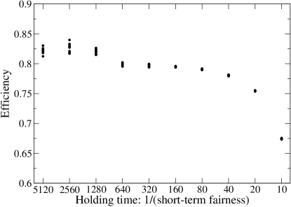
Figure 1: Efficiency vs. short-term fairness tradeoff in a 3-link linear network. Algorithm parameters: $b[t]=0.001$, $W(x)=x$, $V=1$, $\epsilon\lambda^{\max}=0.1$.

References

- [1] L. Tassiulas and A. Ephremides, “Stability properties of constrained queueing systems and scheduling for maximum throughput in multihop radio networks,” IEEE Transactions on Automatic Control, vol. 37, no. 12, pp. 1936–1949, December 1992.
- [2] Y. Yi, A. Proutiere, and M. Chiang, “Complexity in wireless scheduling: Impact and tradeoffs,” in Proceedings of ACM Mobihoc, 2008.
- [3] L. Jiang and J. Walrand, “A distributed algorithm for optimal throughput and fairness in wireless networks with a general interference model,” in Proc. of Allerton conference, September 2008.
- [4] S. Rajagopalan and D. Shah, “Distributed algorithm and reversible network,” in Proc. of CISS, March 2008.
- [5] J. Liu, Y. Yi, A. Proutiere, M. Chiang, and V. Poor, “Maximizing utility via random access without message passing,” Microsoft Research 2008-128, Tech. Rep., September 2008.
- [6] B. Hajek, “Cooling schedules for optimal annealing,” Mathematics of Operations Research, vol. 13, pp. 311–329, May 1988.
- [7] M. Durvy and P. Thiran, “Packing approach to compare slotted and non-slotted medium access control,” in Proc. of IEEE Infocom, 2006.
- [8] V. Borkar, “Stochastic approximation with controlled markov noise,” Systems and control letters, vol. 55, pp. 139–145, 2006.
- [9] ——, Stochastic Approximation, a Dynamical Systems Viewpoint. Hindustan Book Agency (Cambridge University Press), 2008.
- [10] M. Benaim, “A dynamical system approach to stochastic approximation,” SIAM J. on control and optimization, vol. 34, pp. 437–472, 1996.
- [11] J. Ni and R. Srikant, “Distributed CSMA/CA algorithms for achieving maximum throughput in wireless networks,” in Proc. of ITA, Feb 2009.
- [12] F. Baccelli and P. Bremaud, Elements of Queueing Theory. Springer Verlag, Applications of Mathematics, 1994.