Activation of the Blandford-Znajek mechanism in collapsing stars

Abstract

Collapse of massive stars may result in formation of accreting black holes in their interior. The accreting stellar matter may advect substantial magnetic flux onto the black hole and promote release of its rotational energy via magnetic stresses (the Blandford-Znajek mechanism). In this paper we explore whether this process can explain the stellar explosions and relativistic jets associated with long Gamma-ray-bursts. In particularly, we show that the Blandford-Znajek mechanism is activated when the rest mass-energy density of matter drops below the energy density of magnetic field in the very vicinity of the black hole (within its ergosphere). We also discuss whether such a strong magnetic field is in conflict with the rapid rotation of stellar core required in the collapsar model and suggest that the conflict can be avoided if the progenitor star is a component of close binary. In this case the stellar rotation can be sustained via spin-orbital interaction. In an alternative scenario the magnetic field is generated in the accretion disk but in this case the magnetic flux through the black hole ergosphere is not expected to be sufficiently high to explain the energetics of hypernovae by the BZ mechanism alone. However, this energy deficit can be recovered via additional power provided by the disk.

1 Introduction

The most popular model for the central engines of long Gamma-ray-burst (GRB) jets is based on the “failed supernova” scenario of stellar collapse, or “collapsar”, where the iron core of progenitor star forms a BH (Woosley, 1993). If the specific angular momentum in the equatorial part of progenitor exceeds that of the marginally bound orbit of the BH then the collapse becomes highly anisotropic. While in the polar region it may proceed more or less uninhibited, at least for a while, the equatorial layers form dense and massive accretion disk. The gravitational energy released in this disk can be very large, more then sufficient to overturn the collapse of outer layers and drive GRB outflows (MacFadyen & Woosley, 1999). A similar configuration can be produced via inspiraling of a BH or a neutron star into the companion star during the common envelope phase of a close binary (Tutukov & Iungelson, 1979; Frayer & Woosley, 1998; Zhang & Fryer, 2001). In any case, the observed duration of long GRBs, between 2 and 1000 seconds, imposes a strong constraint on the size of progenitors - their light crossing time should be significantly shorter then the burst duration. This implies that the progenitors must be compact stars stripped of their hydrogen envelopes. This conclusion agrees with the absence of hydrogen lines in the spectra of supernovae identified with GRBs (Moreover, since some of these supernovae are of Type Ic their progenitors may have lost their helium envelopes as well.). Massive solitary stars can lose their envelopes via strong stellar winds. However, this may lead to unacceptably low rotation rates by the time of stellar collapse (Heger et al., 2005). In the case of binary system the loss of envelope can be caused by the gravitational interaction with companion.

The currently most popular mechanism of powering GRB jets is the heating via annihilation of neutrinos and anti-neutrinos produced in the disk (MacFadyen & Woosley, 1999). The energy deposited in this way is a strong function of the mass accretion rate which must be above $\simeq 0.05M_{\odot}\mbox{s}^{-1}$ in order to agree with the observational constraints on the energetics of GRBs (Popham et al., 1999). Such high accretion rates can be provided in the collapsar scenario and the numerical simulations by MacFadyen & Woosley (1999) and Aloy et al. (2000) have demonstrated that sufficiently large energy deposition in the polar region above the disk may indeed result in fast collimated jets. However, we have to wait for simulations with proper implementation of neutrino transport before making final conclusion on the suitability of this model – the long and complicated history of numerical studies of neutrino-driven supernova explosions teaches us to be cautious. The first attempt to include neutrino transport in collapsar simulations was made by Nagataki et al. (2007) and they did not see neutrino-driven polar jets - the heating due to neutrino annihilation could not overcome the cooling due to neutrino emission. In any case, it is unlikely that this model can explain the bursts that are longer than $100$s as by this time the mass accretion rate is expected to drop significantly. For example the accretion rate in the simulations by MacFadyen & Woosley (1999) has already drifted below the critical $\dot{M}\simeq 0.05M_{\odot}\mbox{s}^{-1}$ by $t=20$s.

The two alternatives to the neutrino mechanism which are also frequently mentioned in connection with GRBs are the magnetic braking of the accretion disk (Blandford & Payne, 1982; Narayan et al., 1992; Meszaros & Rees, 1997; Proga et al., 2003; Uzdensky & MacFadyen, 2006) and the magnetic braking of the central black hole (Blandford & Znajek, 1977; Meszaros & Rees, 1997; Lee et al., 2000; McKinney, 2006; Barkov & Komissarov, 2008a, b).

A number of groups have studied the potential of magnetic mechanism in the collapsar scenario using Newtonian MHD codes and implementing the Paczynski-Witta potential in order to approximate the gravitational field of central BH (Proga et al., 2003; Fujimoto et al., 2006; Nagataki et al., 2007). In this approach it is impossible to capture the Blandford-Znajek effect and only the magnetic braking of accretion disk can be investigated. The general conclusion of these studies is that the accretion disk can launch magnetically-driven jets provided the magnetic field in the progenitor core is sufficiently strong. This field is further amplified in the disk, partly due to simple winding of poloidal component and partly due to the magneto-rotational instability (MRI), until the magnetic pressure becomes very large and pushes out the surface layers of the disk. In particular, Proga et al. (2003) studied the collapse of a star with a similar structure to that considered MacFadyen & Woosley (1999) and with purely monopole initial magnetic field of strength $B=2\times 10^{14}$G at $r=3r_{g}$. The corresponding total magnetic flux, $\Psi_{h}\simeq 10^{26}\mbox{G}\,\mbox{cm}^{2}$, is in fact within the observational constraints on the field of magnetic stars, including white dwarfs (Schmidt et al., 2003), Ap-stars (Ferrario & Wickramasinghe, 2005) and massive O-stars Donati et al. (2002). They used realistic equation of state and included the neutrino cooling but not the heating. The simulations lasted up to $t\simeq 0.28$s in physical time during which a Poynting-dominated polar jet has developed in the solution. The jet power seemed to show strong systematic decline, from $\simeq 10^{51}\mbox{erg}\,\mbox{s}^{-1}$ down to $\simeq 10^{50}\mbox{erg}\,\mbox{s}^{-1}$ or even less, which might signal transient phenomenon.

Sekiguchi & Shibata (2007) studied the collapse of rotating stellar cores and formation of BHs and their disks in the collapsar scenario using the full GRMHD approximation. Their simulations show powerful explosions soon after the accretion disk is formed and the free falling plasma of collapsing star begins to collide with this disk. However, they did not account for the neutrino cooling and the energy losses due to photo-dissociation of atomic nuclei so these explosions could be similar in nature to the “successful” prompt explosions of early supernova simulations (Bethe, 1990). Mizuno et al. (2004a, b) carried out GRMHD simulations in the time-independent space-time of a central BH. Their computational domain did not capture the BH ergosphere and thus they could not study the role of the Blandford-Znajek effect (Komissarov, 2004a, 2008). In addition, the energy gains/losses due to the neutrino heating/cooling were not included and the equation of state (EOS) was a simple polytrope. The simulations run for a rather short time, $\simeq 280r_{g}/c$ where $r_{g}=GM/c^{2}$, and jets were formed almost immediately, presumably due to the extremely strong initial magnetic field.

The original theory of the Blandford-Znajek mechanism was developed within the framework of magnetodynamics (the singular limit of RMHD approximation where the inertia of plasma particles is fully ignored). The pioneering numerical studies of this mechanism have shown that it can also operate within the full RMHD approximation, at least in the regime where the energy density of matter is much smaller compared to that of the electromagnetic field, and that it can be captured by modern numerical techniques (Komissarov, 2004b; Koide, 2004; McKinney & Gammie, 2004; Nagataki, 2009). However, no systematic numerical study has been carried out in order to establish the exact conditions for activation of the BZ mechanism.

The first simulations demonstrating the potential of the BZ mechanism in the collapsar scenario were carried out by McKinney (2006) who also used simple polytropic EOS and considered purely adiabatic case, but captured the effects of black hole ergosphere. The initial configuration included a torus with poloidal magnetic and a free-falling stellar envelope. The results show ultrarelativistic jets with the Lorentz factor up to 10 emerging from the black hole indicating that the Blandford-Znajek effect may play a key role in the production of GRB jets. Barkov & Komissarov (2008a, b) added a realistic EOS and included the energy losses due to neutrino emission (assuming optically thin regime) and photo-dissociation of nuclei. They also reported the development of relativistic outflows powered by the central black hole via the Blandford-Znajek mechanism (the magnetic braking of accretion disk did not seem to contribute much to the jet power though).

The black hole-driven magnetic stellar explosions and relativistic jets observed in these exploratory computer simulations invite a deeper analysis of this model. Obviously, such an outcome cannot be a generic feature of core-collapse supernovae. Indeed, only a very small fraction of SNe Ib/Ic seem to produce GRBs (Piran, 2005; Woosley & Bloom, 2006). So what are the relevant conditions and can they be reproduced as the results of stellar evolution? These are the main issues we address in this paper.

2 Blandford-Znajek mechanism and GRBs

The rotational energy of Kerr black hole is

$$E_{\mbox{\tiny rot}}=M_{h}c^{2}f_{1}(a)\,\simeq\,1.8\!\times\!10^{54}f_{1}(a)\left(\frac{M_{h}}{M_{\odot}}\right)\mbox{erg},$$ (1)

where

$$f_{1}(a)=1-\frac{1}{2}\left[\left(1+\sqrt{1-a^{2}}\right)^{2}+a^{2}\right]^{1/2},$$

$M_{h}$ is the BH mass and $a\in[0,1)$ is its dimensionless rotation parameter. For $M_{\mbox{\tiny bh}}=2M_{\sun}$ and $a=0.9$ this gives the enormous value of $E_{\mbox{\tiny rot}}\simeq 5\times 10^{53}$erg which is about fifty times higher than the rotational energy of a millisecond pulsar and well above of what is needed to explain the energy of GRBs and associated hypernovae. Even for a relatively slowly rotating black hole with $a=0.1$ this is still a respectable number, $2.3\!\times\!10^{51}$erg. Moreover, because in all versions of the collapsar model the black hole spin is aligned with the spin of accretion disk this energy reserver is continuously replenished via accretion. Thus, as far as the availability of energy is concerned the black hole model looks very promising indeed.

The energy release rate is usually estimated using the Blandford-Znajek power for the case of force-free monopole magnetosphere

$$\dot{E}_{\mbox{\tiny BZ}}=\frac{1}{6c}\left(\frac{\Omega_{h}\Psi_{h}}{8\pi}\right)^{2},$$ (2)

where $\Omega_{h}$ is the angular velocity of the BH and $\Psi_{h}$ is the magnetic flux threading one hemisphere of the BH horizon (Here it is assumed that the angular velocity of the BH magnetosphere $\Omega=0.5\Omega_{h}$.). This formula is quite accurate not only for slowly rotating black holes considered in Blandford & Znajek (1977) but also for rapidly rotating BHs (Komissarov, 2001). In application to the collapsar problem it gives us the following estimate

$$\dot{E}_{\mbox{\tiny BZ}}=1.4\times 10^{51}f_{2}(a)\Psi_{\mbox{\tiny h,27}}^{2}\left(\frac{M_{h}}{M_{\odot}}\right)^{-2}\,\mbox{erg}\,\mbox{s}^{-1},$$ (3)

where

$$f_{2}(a)=a^{2}\left(1+\sqrt{1-a^{2}}\right)^{-2},$$

and $\Psi_{\mbox{\tiny h,27}}=\Psi_{h}/10^{27}\mbox{G}\,\mbox{cm}^{2}$. One can see that the power of BZ-mechanism is rather sensitive to black hole’s mass and magnetic flux. Since, the black hole mass is likely to be $\geq 3M_{\odot}$ the observed energetics of hypernovae and long GRBs requires $\Psi_{\mbox{\tiny h,27}}\simeq 1$. This value is comparable with the maximal surface flux observed in magnetic stars, Ap stars, magnetic white dwarfs, and magnetars (e.g. Ferrario & Wickramasinghe, 2005). Thus, the magnetic field of GRB central engine may well be the original field of the progenitor star.

The estimates (1,3) show that braking of black holes alone can explain the energetics of GRBs and this is why this mechanism is often mentioned in the literature on GRBs. However, there is another issue to take into consideration. The equation (2) is obtained in the limit where the inertia of magnetospheric plasma and, to large degree, its gravitational attraction towards the black hole are ignored. In contrast, the mass density of plasma in the collapsing star may be rather high and has to be taken into account. For example, the magnetohydrodynamic waves may become trapped in the accretion flow and unable to propagate outwards. In such a case, it would not be possible to extract magnetically any of the black hole rotational energy and drive stellar explosion irrespectively of how high this energy is. Since the BZ mechanism can only operate within the black hole ergosphere (e.g. Komissarov, 2004a, 2008), the magnetohydrodynamic waves must at least be able to cross the ergosphere in the outward direction for its activation. This agrees with the conclusion reached in Takahashi et al. (1990) that the Alfven surface of a steady-state ingoing wind must be located inside the ergosphere to have outgoing direction of the total energy flux. Thus we should consider the following condition for activation of the BZ-mechanism in accretion flows: the Alfven speed has to exceed the local free fall speed at the ergosphere,

$$v_{a}>v_{f}.$$

In order to simplify calculations let us apply the Newtonian expressions for both speeds. The Alfven speed is

$$v_{a}^{2}=\frac{B^{2}}{4\pi\rho},$$

where $B$ is the magnetic field strength and $\rho$ is the plasma mass density, whereas the free-fall speed is

$$v^{2}_{f}=\frac{2GM_{h}}{r}.$$

At $r=2r_{g}=2GM/c^{2}$ the local criticality condition reads

$$\beta_{\rho}=\frac{4\pi\rho c^{2}}{B^{2}}<1.$$ (4)

That is the energy density of magnetic field has to exceed that of plasma in the vicinity the black hole.

For spherically symmetric flows the condition $v_{a}>v_{f}$ can be written as a constraint on the mass accretion rate, $\dot{M}$, and the flux of radial magnetic field, $\Psi$,

$$\frac{\Psi}{2\pi r\sqrt{\dot{M}v_{f}(r)}}>1.$$

Since $v_{f}\propto r^{-1/2}$ this condition is bound not to be satisfied at large $r$ but we only need to apply it at the ergosphere. Using $r\simeq 2r_{g}$ we then obtain

$$\kappa>\kappa_{c},$$ (5)

where

$$\kappa=\frac{\Psi_{h}}{4\pi r_{g}\sqrt{\dot{M}c}},$$ (6)

and $\kappa_{c}=1$. In fact, the critical value of $\kappa$ must depend on the black hole spin and tend to infinity for small $a$. The Newtonian analysis cannot capture this effect. The relativistic one, on the other hand, appears rather complicated (Camenzind, 1989; Takahashi et al., 1990). Fortunately, nowadays this issue can be investigated via numerical simulations. Another, interesting and important issue for time-dependent simulations is whether there is only one bifurcation separating solutions with switched-on and switched-off BZ mechanism or the transition is reacher and allows more complicated time-dependent solutions, e.g. quasi-periodic or chaotic ones.

3 Test simulations.

The first type of simulations presented in this paper are designed to test the validity of our arguments behind the criterion for activation of BZ-mechanism which we derived in Sec.2 using a combination of Newtonian and relativistic physics. For this purpose we consider a more or less spherical accretion of cold magnetized plasma with vanishing angular momentum onto a rotating black hole. In order to focus on the MHD aspects of the problem we ignore the microphysics important in the collapsar problem and consider plasma with simplified polytropic EOS.

The main details of our numerical method and various test simulations are described in Komissarov (1999, 2004b, 2006). The only really new feature here is the introduction of HLL-solver which is activated when our linear Riemann solver fails. This usually occurs in regions of relativistically high magnetization where the magnetic energy density exceeds that of matter by more than one order of magnitude or in strong rarefactions. This makes the scheme a little bit more robust though we are still forced to use a “density floor”, that is a lower limit on the value of mass-energy density of matter.

Both in the numerical scheme and throughout this section of the paper we utilize geometric units where $G=c=M_{h}=1$. The Kerr spacetime is described using the Kerr-Schild coordinates so the metric form reads

$$\begin{array}[]{rl}ds^{2}=&g_{tt}dt^{2}+2g_{t\phi}dtd\phi+2g_{tr}dtdr+\\ &g_{\phi\phi}d\phi^{2}+2g_{r\phi}d\phi dr+g_{rr}dr^{2}+g_{\theta\theta}d\theta^{2},\end{array}$$ (7)

where

$$g_{tt}=\zeta-1,\quad g_{t\phi}=-\zeta a\sin^{2}\!\theta,\quad g_{tr}=\zeta,$$

$$g_{\phi\phi}=\Sigma\sin^{2}\theta/A,\quad g_{r\phi}=-a\sin^{2}\theta(1+\zeta),\quad$$

$$g_{rr}=1+\zeta,\quad g_{\theta\theta}=A,$$

and

$$A = r^{2}+a^{2}\cos^{2}\!\theta,$$

$$\zeta = 2r/A,$$

$$\Sigma = (r^{2}+a^{2})^{2}-a^{2}\Delta\sin^{2}\!\theta,$$

$$\Delta = r^{2}+a^{2}-2r.$$

3.1 Setup

The initial solution has to describe both the flow and the magnetic field. In this case the flow is given by the steady-state solution for unmagnetised cold plasma (dust). At infinity it is spherically symmetric and has vanishing specific angular momentum and radial velocity. The components of 4-velocity of this flow in the coordinate basis of Kerr-Schild coordinates, $\{\partial_{\nu}\}$, are

$$\begin{array}[]{l}u^{t}=1+\zeta\eta/(1+\eta);\\ u^{\phi}=-a/(A(1+\eta));\\ u^{r}=-\zeta\eta;\\ u^{\theta}=0,\end{array}$$ (8)

where $\eta=\sqrt{(r^{2}+a^{2})/2r}$ and its rest mass density is

$$\rho=\rho_{+}\left(\frac{r_{+}}{r}\right)\frac{1}{\eta}$$ (9)

where $\rho_{+}$ is the rest mass density at the outer event horizon radius (see Appendix A).

The initial magnetic field is radial with monopole topology

$$\begin{array}[]{l}B^{\phi}=aB^{r}(A+2r)/(A\Delta+2r(r^{2}+a^{2}));\\ B^{r}=B_{0}\sin\theta/\sqrt{\gamma};\\ B^{\theta}=0.\end{array}$$ (10)

The azimuthal component is introduced in order to ensure that the electromagnetic fluxes of energy and angular momentum vanish (see Appendix B) and, thus, the initial magnetic configuration is more or less dynamically passive.

The two-dimensional axisymmetric computational domain is $(r_{0}\!<\!r\!<\!r_{1})\times(0\!<\!\theta\!<\!\pi)$, where $r_{0}=1+0.5\sqrt{1-a^{2}}$ and $r_{1}=500$. Notice that the inner boundary is inside of the outer event horizon, $r_{+}=1+\sqrt{1-a^{2}}$. This can be done because of the non-singular nature of the horizon in the Kerr-Schild coordinates. The computational grid is uniform in $\theta$, where it has 100 cells, and almost uniform in $\log r$, where it has 170 cells. The metric cell sizes are the same in both directions. The grid is divided into rings such that for any ring the metric size of its outer cells is twice that of its inner cells. The solution on each ring is advanced with its own time step, the outer ring time step being twice that of the inner ring. At the interface separating cells of different rings the conservation of mass, energy, and momentum and magnetic flux is ensured via simple averaging procedure.

At the inner boundary, $r=r_{0}$, we impose the “non-reflective” free-flow boundary conditions. The use of these conditions is justified by the fact that this boundary lies inside the outer event horizon in the region where all physical waves move inwards. At the outer boundary, $r=r_{1}$ we fix the flow parameters corresponding to the initial solution. In all runs the simulations are terminated well before any strong perturbation generated near the centre reaches this boundary. At the polar axis, $\theta=0,\pi$, the boundary conditions are dictated by the axial symmetry. Namely, quantities that do not vanish on the axis are reflected without change of sign, whereas quantities that vanish on the axis are reflected with change of sign.

We consider models which differ only by the rotation rate of black hole, $a$, and the mass accretion rate, $\dot{M}$. For each value of $a$, we first deal with the model with $\kappa\simeq 1$. Depending on whether the BZ-mechanism is activated in this model or not we either increase or reduce $\rho_{+}$ (and hence $\dot{M}$) by the factor of three and compute another model. We proceed in this fashion until the solution becomes qualitatively different. Then we compute one more model based on the mean value of $\rho_{+}$ for the previous two models. After that we select the closest two models with qualitatively different solutions and show them on the bifurcation diagram summarising the results of our study.

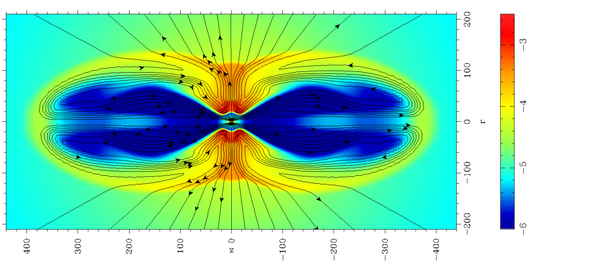
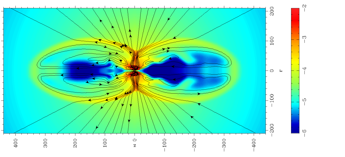
Figure 1: Free-fall accretion of cold plasma with zero angular momentum onto a Kerr black hole ($a=0.9$); the global structure. The colour images show $\log_{10}\rho$ in dimensionless units and the contours show the magnetic field lines ( To be more specific the contours show the levels of poloidal magnetic flux function, $\Psi$. At any point $(r,\theta)$ this function gives the magnetic flux through the axisymmetric loop or radius $r$ passing through this point.). Top panel: model with the activation parameter $\kappa=1.2$ at time $t=2000r_{g}/c$. Middle panel: model with $\kappa=1.6$ and monopole magnetic field at time $t=1000r_{g}/c$. Bottom panel: model with $\kappa=1.6$ and split-monopole magnetic field at time $t=1600r_{g}/c$. The unit of length is $r_{g}$.

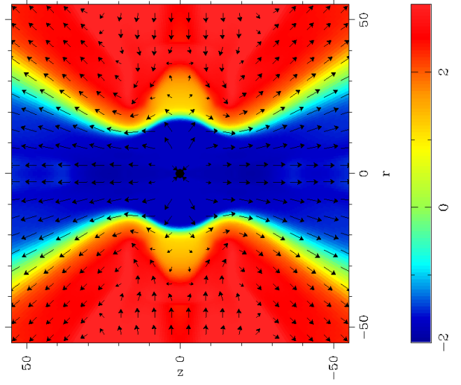
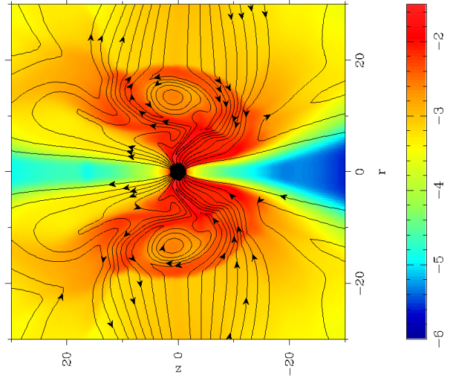
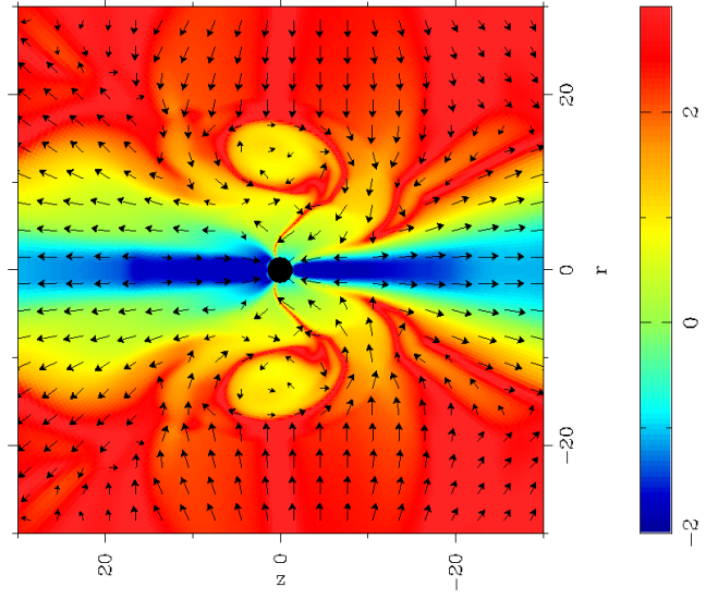
Figure 2: Free-fall accretion of cold plasma with zero angular momentum onto a Kerr black hole ($a=0.9$); the central regions. The top panels show the model with $\kappa=1.2$ at $t=2000r_{g}/c$; the middle panels show the model with $\kappa=1.6$ and monopole magnetic field at $t=1000r_{g}/c$, the bottom panels show the model with $\kappa=1.6$ and split-monopole magnetic field at $t=1600r_{g}/c$. The left panels show the rest mass density distribution ($\rho$ for the top panel and $\log_{10}\rho$ for others) and the magnetic field lines. The right panels show the ratio of the proper rest mass and magnetic energy densities, $\log_{10}\beta_{\rho}$, and the velocity field (the length of velocity arrow is proportional to the square root of speed.).

3.2 Results

The simulations do confirm the anticipated bifurcation and show that for a wide of parameter $a$ the critical value of $\kappa$ is indeed close to unity. For example, the model with $a=0.9$ and $\kappa=1.2$ is qualitatively different from the model the model with $a=0.9$ and $\kappa=1.6$. The first model quickly settles to a steady state accretion solution (see the top panels of fig.1 and fig.2). In fact, on the large-scales, this solution is almost indistinguishable from the initial solution. On the small scales, near the event horizon, the differences become more pronounced. In particular, a stationary accretion shock appears just outside of the ergosphere. It is responsible for the jump in the rest mass density and the kinks of magnetic field lines seen in the top left panel of fig.2. Inside the ergosphere the magnetization parameter $\mu$ is larger than unity but only just. The magnetic field lines show no rotation and thus the BZ-mechanism remains completely switched-off.

In contrast, the model with $a=0.9$ and $\kappa=1.6$ exhibits powerful bipolar outflow which drives a blast wave into the accreting flow (see the middle panel of fig.1). This blast waves overturns the accretion both in the polar and in the equatorial direction. The black hole develops highly rarefied magnetosphere (see the middle panels of fig.2) which rotates with about half of black hole’s angular velocity. The shocked plasma of accretion flow is prevented from accretion onto the black hole – instead it participates in the large scale circulations above and below the equatorial plane. The unphysical monopole configuration of magnetic field set for this model prevents any escape of magnetic flux from the black hole. This ensures operation of the BZ-mechanism even if the confining accreting envelope is fully dispersed into the surrounding space.

For a more realistic dipolar configuration one would expect at least partial escape of magnetic flux once the outflow is developed and thus less power in the outflow. However, this is unlikely to effect the value of $\kappa_{c}$. Indeed, consider the case with monopole field where the BZ-mechanism remains switched off. Then, change the polarity of magnetic field lines in the northern hemi-sphere. Because the speeds of MHD waves and the magnetic stresses remain invariant under change of magnetic polarity this will have no effect on the flow. For the very same reason, we expect activation of the BZ mechanism for exactly the same value of $\kappa$ in both magnetic configurations. In order to verify this conclusion we computed models with the initial magnetic field of split-monopole topology and the results fully agree with the expectations – the critical value of $\kappa$ remains unaffected but the power of BZ-mechanism is reduced due partial escape of magnetic flux from the black hole. The bottom panel of fig.1 shows the large scale flow developed in the model with $a=0.9$, $\kappa=1.6$, and split-monopole initial magnetic field. The flow pattern is very similar to that of the model with monopole field but the expansion rate is noticeable lower, approximately by the factor of 1.8 in the polar direction and even more in the equatorial direction. The bottom panels of fig.2 show the inner region of this model. One can see that the accretion is no longer fully halted – the accreting plasma finds its way into the black hole in the equatorial zone and the black hole magnetosphere is confined only to the polar region of the funnel shape.

The results for $a=0.9$ show that not only there is a bifurcation between the regimes with switched-on and switched-off BZ process but also that the critical value of the control parameter $\kappa$, and hence $\beta_{\rho}$, is indeed close to unity at least for rapidly rotating black holes. The results of our parametric study, summarised in fig.3, show that in fact $\kappa_{c}(a)$ is a relatively weak function of $a$. It is confined within the range $(1,2)$ for $0.2<a<1.0$.

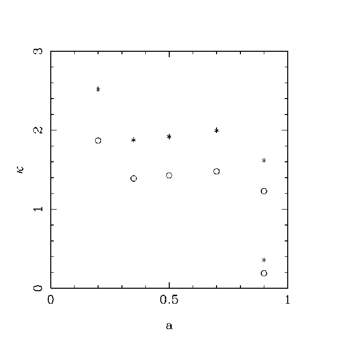
Figure 3: The bifurcation diagram. The stars show the models with the lowest value of $\kappa$ which still show activation of the BZ mechanism. The circles show models with the highest value of $\kappa$ where the BZ mechanism remains turned off. The pair of points with $a=0.9$ in the right bottom corner of the diagram correspond to proper collapsar simulations. The other points show the results for test simulations.

4 Collapsar simulations

The test simulations described in Sec.3 allow us to determine the basic criteria for activation of the BZ mechanism in principle. However, their set-up is rather artificial as in many astrophysical applications the accreting plasma has sufficient angular momentum to ensure formation of accretion disk and thus to render the approximation of spherical accretion unsuitable. This anisotropy of mass inflow is likely to make the integral activation condition (5) less helpful. On the other hand, one would expect the local condition condition (4) to be more or less robust. In order to check this we analysed the results obtained in our current numerical study of magnetic collapsar model.

4.1 Computational grid and boundary conditions

Like in the test simulations we use the Kerr metric in Kerr-Schild coordinates, $\{\phi,r,\theta\}$. We selected $M_{\mbox{\tiny h}}=3M_{\sun}$ and the rather optimistic value of $a=0.9$ for the central black hole. The two-dimensional axisymmetric computational domain is $(r_{0}\!<\!r\!<\!r_{1})\times(0\!<\!\theta\!<\!\pi)$, with $r_{0}=(1+0.5\sqrt{1-a^{2}})\;r_{g}=5.4\,$km and $r_{1}=5700\;r_{g}=25000\,$km. The computational grid is of the same type as in the test simulations (Sec.3.1) but with more cells, $450\times 180$. The boundary conditions are also the same as in the test simulations.

4.2 Microphysics

For these simulations we use realistic equation of state (EOS) that takes into account the contributions from radiation, lepton gas including pair plasma, and non-degenerate nuclei (hydrogen, helium, and oxygen). This is achieved via incorporation of the EOS code HELM (Timmes & Swesty, 2000), which can be downloaded from the web-site http://www.cococubed.com/code_pages/eos.shtml.

The neutrino cooling is computed assuming optically thin regime and takes into account URCA-processes (Ivanova et al., 1969), pair annihilation, photo-production, and plasma emission (Schinder et al., 1987), as well as synchrotron neutrino emission (Bezchastnov et al., 1997). In fact, URCA-processes strongly dominate over other mechanisms in this problem. Photo-disintegration of nuclei is included via modification of EOS following the prescription given in Ardeljan et al. (2005). The equation for mass fraction of free nucleons is adopted from Woosley & Baron (1992). We have not included the radiative heating due to annihilation of neutrinos and antineutrinos produced in the accretion disk mainly because this requires elaborate and time consuming calculations of neutrino transport.

4.3 Model of collapsing star

The collapsing star is introduced using the simple free-fall model by Bethe (1990). In this model it is assumed that immediately before the collapse the mass distribution in the star satisfies the law $\rho r^{3}=$const and that the infall proceeds with the free-fall speed in the gravitational field of the central black hole. This gives us the following radial velocity

$$v^{r}_{\mbox{\tiny ff}}=(2GM/r)^{1/2}$$ (11)

and mass density

$$\rho=C_{1}\times 10^{7}\left(\frac{t_{s}}{1\mbox{~{}s}}\right)^{-1}\left(\frac{r}{10^{7}\mbox{cm}}\right)^{-3/2}\mbox{g~{}cm}^{-3}$$ (12)

for the collapsing star, where $C_{1}$ is a constant that depends on the star mass (Bethe, 1990) and $t_{s}$ is the time since the start of collapse. The corresponding accretion rate and ram pressure are

$$\dot{M}=0.056~{}C_{1}\left(\frac{M}{3M_{\sun}}\right)^{1/2}\left(\frac{t_{s}}{1\,\mbox{s}}\right)^{-1}M_{\sun}\mbox{s}^{-1},$$ (13)

$$p_{\mbox{\tiny ram}}=7.9\times 10^{26}C_{1}\frac{M}{3M_{\sun}}\left(\frac{t_{s}}{1\mbox{~{}s}}\right)^{-1}\left(\frac{r}{10^{7}\mbox{cm}}\right)^{-5/2}\frac{\mbox{g}}{\mbox{cm~{}s}^{2}}$$ (14)

respectively. For a core of radius $r_{c}=10^{9}$cm and mass 3.0$M_{\sun}$ the collapse duration can be estimated as $t_{c}=2r_{c}/3v_{\mbox{ff}}\simeq 0.6$s. Since, in this study we explore the possibility of early explosion, that is soon after the core collapse, we set $t_{s}=1$s. Because GRBs are currently associated with more massive progenitors we consider $C_{1}=3,9$. This gives us the accretion rates of $\dot{M}\simeq 0.166M_{\sun}\mbox{s}^{-1}$ and $\dot{M}\simeq 0.5M_{\sun}\mbox{s}^{-1}$ respectively.

On top of this we endow the free-falling plasma with angular momentum and poloidal magnetic field. The angular momentum distribution is

$$l=\sin\theta\left\{\begin{array}[]{lcl}l_{0}(r\sin\theta/r_{l})^{2}&\quad\mbox{if}&r\sin\theta<r_{l}\\ l_{0}&\quad\mbox{if}&r\sin\theta>r_{l}\end{array}\right.,$$ (15)

where $r_{l}=6300$km and $l_{0}=10^{17}\mbox{cm}^{2}\mbox{s}^{-1}$.

4.4 Initial magnetic field

The origin of magnetic field is probably the most important and difficult issue of the magnetic model of GRBs. One possibility is that this field already exists in the progenitor and during the collapse it is simply advected onto the black hole. The recent numerical studies indicate that the poloidal and the azimuthal components of the progenitor field should have similar strengths (Braithwaite & Spruit, 2004). The magnetic flux freezing argument then suggests that during the collapse the poloidal field becomes dominant and thus in our simulations we may ignore the initial azimuthal field. As to the initial poloidal component we adopt the solution for a uniformly magnetized sphere in vacuum. To be more specific, we assume that inside the sphere of radius $r_{m}=4500\,$km the magnetic field is uniform and has strength of either $B_{0}=3\times 10^{9},\,10^{10},$ or $3\times 10^{10}$G, whereas outside it is described by the solution for magnetic dipole. The selected values for the field strength allow to capture the BZ bifurcation. Given the limitations of axisymmetry we can only consider the case of aligned magnetic and rotational axes.

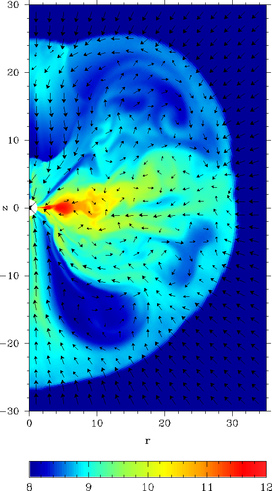
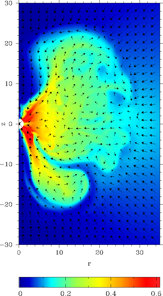
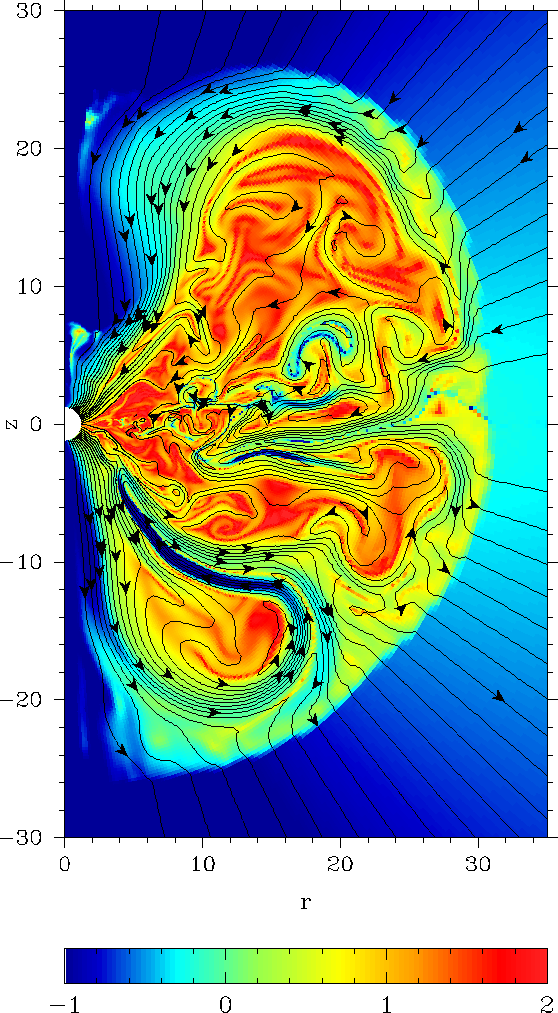
Figure 4: Model B close to the explosion, at $t=237$ms. Top left: $\log_{10}\rho$ and the poloidal velocity; Top right: the angular velocity of plasma and the poloidal velocity; Bottom left: the ratio of azimuthal and poloidal components of magnetic field, $\log_{10}(|\mn@boldsymbol{B}_{\phi}|/|\mn@boldsymbol{B}_{p}|)$, and the magnetic field lines; Bottom right: $\log_{10}\beta_{\rho}$, the magnetic field lines, and the poloidal velocity field. The length of velocity arrows is proportional to the square root of speed.

4.5 Results

Table 1 describes the key parameters of six models investigated in this study and also summarises the outcome of simulations. One of the parameters, $\Psi^{max}$, is the total magnetic flux enclosed by the equator of the uniformly magnetized sphere in the initial solution. Obviously, this gives us the highest magnetic flux that can be accumulated by the black hole in the simulations. Whether this maximum value is actually reached at some point depends on the progenitor rotation. For slow rotation the whole of the uniform magnetized core can be swallowed by the hole before the development of accretion disk. At this point $\Psi_{h}$ equals to $\Psi^{max}$ and then it begins to decline as the result of advection of the oppositely directed parts of dipolar loops (These loops are clearly seen in fig.5). For fast rotation the accretion disk forms before $\Psi_{h}$ reaches $\Psi^{max}$ and after this point the growth of $\Psi_{h}$ slows down noticeably as the disk accretion is much slower compared to the free-fall accretion. Once the oppositely directed parts of magnetic loops begin to cross the accretion shock and enter the turbulent domain that surrounds the disk the annihilation of poloidal magnetic field in this domain becomes an important factor. As the result the maximum value of magnetic flux available in the solution begins to decrease before $\Psi_{h}$ reaches $\Psi^{max}$.

name	$B_{\mbox{\tiny 0,10}}$	$C_{1}$	$\Psi_{\mbox{\tiny 27}}^{max}$	$\kappa_{max}$	Exp	$\Psi_{\mbox{\tiny h,27}}$	$\dot{E}_{\mbox{\tiny 51}}$
A	3	3	19.1	1.07	Yes	11.6	9.6
B	3	9	19.1	0.62	Yes	13.1	12.7
C	1	3	6.67	0.36	Yes	2.80	0.4
D	1	9	6.67	0.21	No
E	0.3	3	1.91	0.11	No
F	0.3	9	1.91	0.06	No

Table 1: Summary of numerical models in collapsar simulations. $B_{0,10}$ is the initial magnetic field strength in units of $10^{10}$G, $C_{1}$ is the density parameter in eq.12, $\Psi_{\mbox{\tiny 27}}^{max}$ is the maximum value of magnetic flux that can be accumulated by the black hole in units of $10^{27}\mbox{G}\,\mbox{cm}^{2}$, $\kappa_{max}$ is the value of $\kappa$ corresponding to $\Psi_{\mbox{\tiny 27}}^{max}$, “Exp” is the explosion indicator, $\Psi_{\mbox{\tiny h,27}}$ is the actual magnetic flux accumulated by the black hole by the time of explosion, $\dot{E}_{\mbox{\tiny 51}}$ is the mean power of the BZ mechanism in units of $10^{51}$erg/s.

$\kappa_{max}$ is the value of parameter $\kappa$ computed using $\Psi^{max}$ instead of the actual value of black hole flux in eq.5. Quick inspection shows that the critical value of $\kappa$ based on the values of $\kappa_{max}$ is about $\kappa_{c}=0.3$ (see models C and D in table 1.), almost five time lower than that in the test simulations of spherical collapse. In fact, the actual value of magnetic flux accumulated by the black hole, $\Pi_{h}$, by the time of explosion is always noticeably lower than $\kappa_{max}$ (see table 1). In model C it is 2.4 times lower thus driving the actual critical value of $\kappa$ down to the value around 0.1. This result is undoubtedly connected to the highly anisotropic nature of the flow in the close vicinity of the black hole that develops in the simulations. Most importantly, there is a clear separation of the mass and magnetic fluxes: while a large fraction of mass is accreted through the accretion disk, the bulk of magnetic field lines connected to the black hole occupy the space above (and below) the disc (see fig.4).

All models considered in this study first pass through the passive phase of almost spherical accretion. During this phase the black hole accumulates magnetic flux but as $\Psi^{max}$ is not sufficiently high the Blandford-Znajek mechanism remains switched-off. Then, as the angular momentum of plasma approaching the black hole exceeds that of the marginally bound orbit, the accretion disk forms in the equatorial plane and an accretion shock separates from its surface. This shock is best seen in the density plot of fig.4 where it appears as a sharp circular boundary between the light blue and dark blue areas of radius $\simeq 30r_{g}\simeq 135$km. In fact, the accretion shock oscillates in a manner reminding the oscillations found earlier in supernova simulations (e.g. Blondin et al., 2003; Buras et al., 2006; Scheck et al., 2008), as well as in simulations of accretion flows onto black holes (Nagakura & Yamada, 2009), and attributed to the so-called Stationary Accretion Shock Instability (SASI). Most likely, the physical origin of shock oscillations in our simulations is the same but we have not explored this issue in details.

During this second phase the differential rotation results in winding up of the magnetic field in the disk and its corona where the azimuthal component of magnetic field begins to dominate (top-right and bottom-left panels of fig.4). The corona acts as a “magnetic shield” deflecting the plasma coming at intermediate polar angles towards either the equatorial plane or the polar axis (see fig.4). In models D,E and F the second phase continues till the end of run and the Blandford-Znajek process remains switch-off permanently. There are no clear indications suggesting that this phase may end soon although the accretion disk grows monotonically in radius and this may eventually bring about a bifurcation.

In models A,B,C after several oscillations the solution enters the third phase which is characterized by a non-stop expansion of the accretion shock which then turns into a blast wave. During this transition the black hole develops a low mass density magnetosphere which occupies the axial funnel through which the rotational energy of the black hole is transported away away in the form of Poynting flux and powers the blast wave. The typical large-scale structure of the the solution during the third phase is shown in fig.5 (see also Barkov & Komissarov (2008a) ). It is rather similar to the structure observed in the simulations of spherical accretion in the case of split-monopole magnetic field (see Sec.3.2).

Figure 4 shows the solution for model B at time $t=237$ms, which is close to the end of the second phase, and helps to understand how exactly the BZ mechanism is activated in our simulations. At this stage, the accretion disk is well developed and accounts for $\simeq 50-60\%$ of mass flux through the event horizon whereas most of the magnetic field lines threading the horizon avoid both the disk and corona that surrounds the disk and contains predominantly azimuthal magnetic field. The strong turbulent motion in the disk and its corona must be the reason for this expulsion of magnetic flux (Zel’dovich, 1957; Rädler, 1968; Tao et al., 1998). In any case, the observed separation of magnetic and mass fluxes results in a rather inhomogeneous magnetization of plasma near the black hole. Most importantly, there are regions that have much higher local magnetization compared to the case of spherical accretion with the same value of integral control parameter $\kappa$.

Moreover, the magnetic shield action of the disk corona can promote further local increase of magnetization. Indeed, the corona can deflect plasma passing through the accretion shock at intermediate latitudes in the direction which does not necessarily coincide with the local direction of the magnetic field. For example, in figure 4 the stagnation point of post-shock flow in the upper hemisphere is located at $(r,z)\simeq(25,20)r_{g}$ whereas the separation between the magnetic field lines connected to the hole and to the disk occurs at much lower latitude, around $(r,z)=(28,10)r_{g}$. Thus, the direct mass loading of the field lines entering the shock between these points with is currently suspended. On the other hand, at the other end of these field lines, where they penetrate the event horizon, their unloading continues as usual. As the result, the magnetization along these lines increases allowing to reach the local criticality condition, $\beta_{\rho}<1$ (see the intense blue regions in the left panel of fig.4). Once this condition is satisfied the BZ mechanism turns on, at this point only very locally and the initial rotation rate of the field lines is significantly lower then $0.5\Omega_{h}$. However, an additional magnetic energy is now being pumped into the shield via the BZ mechanism promoting its expansion and increasing its efficiency as a flow deflector. This causes further increase of the magnetization at its base, further increase of magnetosphere’s rotation rate and thus higher BZ power and so on. The process develops in a runaway fashion.

Figure 5: Model B soon after the explosion. The figure shows the solution at $t=332$ms. The colour image gives $\log_{10}\rho$ and the contours show the magnetic field lines.

Figure 6 shows the magnetization parameter $\beta_{\rho}$ at $r=2r_{g}$ as a function of the polar angle for model B (at the same time as in fig.4) and for model D at a similar time. One can see that for model D the magnetization is lower. In fact, the local criticality condition, $\beta_{\rho}<1$, is not satisfied anywhere for this model and this explains why the explosion is not produced in this model.

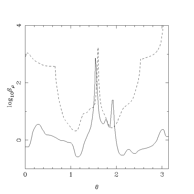
Figure 6: The magnetization parameter $\beta_{\rho}=4\pi\rho c^{2}/B^{2}$ at $r=2r_{g}$ for models B at $t=237$ms (solid line) and D at $t=360$ms (dashed line).

5 Discussion

5.1 The strength and origin of magnetic field.

There seems to be only two possible origins for the magnetic field in the collapsar problem. Either this is a fossil field of the progenitor star of the field generated in the accretion disk and its corona. Here we consider both possibilities.

The blunt application of the integral condition (5) for activation of the Blandford-Znajek mechanism gives us the critical value of magnetic flux accumulated by the black hole

$$\Psi_{h,c}=4.3\times 10^{28}\left(\frac{M_{h}}{3M_{\odot}}\right)\left(\frac{\dot{M}\mbox{s}}{M_{\odot}}\right)^{1/2}\!\!\mbox{G}\,\mbox{cm}^{2}.$$

Although the strength of magnetic field in the interior of massive stars which end up as failed supernovae is not known this is uncomfortably high compared to fluxes deduced from the observations of “magnetic stars” and rises doubts about the fossil hypothesis. However, the actual values of the critical magnetic flux found in our simulations are significantly lower. As we have already commented in Sec.4 this is due to the anisotropy of accretion in the collapsar model. This anisotropy is expected to increase with time as more distant parts of the progenitor with higher angular momentum enter the accretion shock (we could not study this late phase of the collapse, $t\gg 1\,$s, because of various technical issues.). Due to the higher angular momentum the predominant motion downstream of the shock will be towards the equator and this should result in (i) further reduction of the mass flux and the ram pressure of accreting plasma in the polar region and (ii) more effective mass-unloading of magnetic field lines entering the black hole (see Sec.4.5). Both effects promote higher plasma magnetization in the polar region around the black hole which may eventually exceed the local criticality condition (4) even in models with $\Psi_{h}<10^{27}\mbox{G}\mbox{cm}^{2}$, making the fossil hypothesis more plausible.

Our results seem at odds with the Newtonian simulations by Proga et al. (2003) who obtain magnetically driven explosions powered by the disk wind already within $300\,$ms in physical time since the start of simulations for a model with similar mass accretion rate, $\dot{M}\simeq 0.29M_{\odot}/$s, but much lower magnetic field, $\Psi\simeq 10^{26}\mbox{G}\,\mbox{cm}^{2}$. Since their initial model is similar to that of MacFadyen & Woosley (1999) the difference cannot be attributed to the development of highly rarefied polar channel seen in the simulations of MacFadyen & Woosley (1999) as this occurs only several seconds later. Other possible reasons include differences in the framework, details of the initial solutions, resolution, implementation of microphysics etc. Hopefully, simulations by other groups will soon clarify this issue.

Another factor that is likely to reduce the constraint on the strength of the fossil field, and the one that is completely ignored in our simulations, is the plasma heating due to neutrino-antineutrino annihilation. In the most extreme scenario this heating completely overpowers accretion in the polar direction and drives a relativistic GRB jet (MacFadyen & Woosley, 1999). Although this is an attractive model of GRB explosions by itself we also note that the creation of low density funnel in this model helps to activate the BZ mechanism along the magnetic field lines that are advected inside this funnel. Thus, the neutrino heating and BZ mechanism may work hand in hand in driving GRBs and hypernovae.

Even in failed supernovae the stellar core collapse does not lead directly to formation of a black hole but still proceeds through the proto-neutron star (PNS) phase first. If the period of PNS is very short, around several millisecons, its rotational energy is sufficient to strongly modify the direction of collapse and the initial conditions for the black hole phase. In particular, the magnetic stresses due to either fossil or MRI-generated magnetic field can drive powerful bipolar outflows (Moiseenko et al., 2006; Obergaulinger et al., 2006; Burrows et al., 2007). As reported by Burrows et al. (2007) these outflows can coexist with equatorial accretion and may not be able to prevent eventual collapse of PNS. However, they certainly overcome accretion in the polar direction and create favorable conditions for activation of the BZ mechanism. The very fast rotation of progenitor’s Fe core required in this scenario, with the period around few seconds, is unlikely to be achieved in stars with strong fossil magnetic field (see Sec.5.2).

A related issue is whether a significant fraction of fossil magnetic flux available in the progenitor can actually be accumulated by the black hole. The traditional viewpoint is that the inward advection of magnetic field in accretion disk is effective and can result in build-up of poloidal magnetic field up to the equipartition with the disk gas pressure (Bisnovatyi-Kogan & Ruzmaikin, 1974, 1976; Blandford & Znajek, 1977; Macdonald & Thorne, 1982; Begelman et al., 1984). On the other hand, it has also been argued that in standard viscosity driven accretion disk the turbulent outward diffusion of poloidal field may easily neutralise the inward advection well before it reaches the equipartition strength(Lubow et al., 1994; Heyvaerts et al., 1996; Ghosh & Abramowicz, 1997; Livio et al., 1999). However, the disk angular momentum can also be removed by magnetic stresses via interaction with the disk corona and wind and this may change the balance in favour of the inward accretion of poloidal magnetic flux (Spruit & Uzdensky, 2005; Robstein & Lovelace, 2008). This has been demonstrated in recent 3D Newtonian simulations of radiatively inefficient accretion disks where the poloidal magnetic field reached the equipartition strength near the central “black hole”(Igumenshchev, 2008). In our simulations, a significant fraction of black hole’s magnetic flux is accumulated before the development of accretion disk. However, the flux does not escape after the disk is formed. On the contrary, it keeps increasing until the oppositely directed magnetic field lines begin to enter the accretion shock. Thus, our results are in agreement with those by Igumenshchev (2008) and suggest strong magnetic interaction between the disk and its corona/wind.

The alternative origin of magnetic field is via dynamo process in the turbulent accretion disk. In this case the saturated equilibrium magnetic field strength can be estimated from the energy equipartition argument

$$\frac{B_{t}^{2}}{8\pi}\simeq\rho\frac{v_{t}^{2}}{2},$$ (16)

where $B_{t}$ and $v_{t}$ are the turbulent magnetic field and velocity respectively. However, the typical scale of this field is rather small, of the order of the disk hight, $h\ll r_{g}$. When magnetic loops of such small scale are advected onto the black hole one would expect quick, on the time scale of $r_{g}/c$, reconnection and annihilation of magnetic field, resulting in low residual magnetic flux penetrating the black hole. Tout & Pringle (1996) argued that similar reconnection processes in the disk corona may lead to inverse cascade of magnetic energy on scales exceeding $h$. The expected spectrum in this range is $B_{\lambda}\propto 1/\lambda$ and thus on the scale of $r_{g}$ one could find the regular magnetic field of strength

$$B_{p}\simeq\frac{h}{r_{g}}B_{t}.$$

The standard theory of $\alpha$-disks gives

$$v_{t}\simeq\alpha\Omega_{k}h,$$

where $\Omega$ is the Keplerian frequency, $h$ is the half-thickness of the disk and $\alpha=0.1\div 0.01$ is a free parameter of this theory. According to the theory of thin neutrino cooled accretion disks by Popham et al. (1999)

$$\frac{h}{r}=0.09\!\left(\frac{\alpha}{0.1}\right)^{\!0.1}\!\!\left(\frac{M_{h}}{M_{\odot}}\right)^{\!-0.1}\!\!\left(\frac{r}{r_{g}}\right)^{\!0.35}$$

and

$$\rho=2.4\times 10^{15}\!\left(\frac{\alpha}{0.1}\right)^{\!-1.3}\!\!\left(\frac{M_{h}}{M_{\odot}}\right)^{\!\!-1.7}\!\!\!\left(\frac{r}{r_{g}}\right)^{\!\!-2.55}\!\!\!\left(\frac{\dot{M\mbox{s}}}{M_{\odot}}\right)\frac{\mbox{g}}{\mbox{cm}^{3}}.$$

Putting all these equations together we find the typical black hole magnetic flux

$$\Psi_{h}=3\times 10^{26}\!\left(\frac{\alpha}{0.1}\right)^{\!0.55}\!\!\left(\frac{M_{h}}{M_{\odot}}\right)^{\!0.95}\!\!\left(\frac{\dot{M\mbox{s}}}{M_{\odot}}\right)^{\!0.5}\mbox{G}\,\mbox{cm}^{2}.$$ (17)

The corresponding power of BZ mechanism is

$$\dot{E}_{\mbox{\tiny BZ}}\simeq 1.3\times 10^{50}f_{2}(a)\left(\frac{\alpha}{0.1}\right)^{1.1}\left(\frac{\dot{M}\mbox{s}}{M_{\odot}}\right)\,\mbox{erg}\,\mbox{s}^{-1}$$ (18)

almost independently on the black hole mass. One can see that even for maximally rotating black holes one should not expect much more than $10^{51}$erg from a collapse of a $10M_{\odot}$ progenitor. On the other hand, in this model one should expect a much more powerful magnetically driven wind from the accretion disk (Livio et al., 1999). Mass loading of this wind is likely to be much higher due to the processes similar to solar coronal mass injections are the terminal Lorentz factors are not expected to be as high as required from the GRB observations. However, the disk wind could be responsible for the $\sim\!10^{52}$ergs required to drive hypernova. Having said that, we need to warn that the above equations are purely Newtonian and thus their application to the very vicinity of black hole may introduce large errors. Moreover, the current theory of magnetic dynamo in accretion disks can hardly be called well developed and so one could expect few surprises as our understanding of the dynamo improves. Finally, the above picture is in conflict with our numerical models, particularly those which do not show BZ driven explosions. It is difficult to pin down the exact reasons for this but the key issues are likely to be the condition of axisymmetry and numerical resolution.

5.2 The nature of rotation

With a typical rotation rate of $200\,$km/s on the zero-age main-sequence (e.g. Penny, 1996; Howarth et al., 1997) the standard evolutionary models of solitary stars predict very rapid rotation of stellar cores by the time of collapse (Heger et al., 2000; Hirschi et al., 2004, 2005). According to these models the typical periods of newly born pulsars in successful supernovae are around one millisecond and “failed supernovae” conceive rapidly rotating black holes with accretion disks, as required for GRBs. These results, however, contradict to observations which clearly indicate that young millisecond pulsars and GRBs are much more rare.

When the magnetic torque due to the relatively weak magnetic field generated via the Tayler-Spruit dynamo (Tayler, 1973; Spruit, 2002) is included in the evolutionary models they result in significant spin down of stellar cores during the red giant phase and during the intensive mass loss period characteristic for massive stars at the Wolf-Rayet phase (Heger et al., 2005). As the result the predicted rotation rates for newly born pulsars come to agreement with the observations but on the other hand, the core rotation becomes too low compared to what is required for the collapsar model of GRBs (Heger et al., 2005). Recently, it was proposed that low metalicity could be the factor that allows to reduce the efficiency of magnetic braking in GRB progenitors (Woosley & Heger, 2006; Yoon et al., 2006). On one hand, the mass-loss rate of WR-stars decreases significantly with metalicity. On the other hand, the evolutionary models of Woosley & Heger (2006) show that low metalicity stars rotating close to break-up speed may become fully convective, chemically homogeneous, and by-pass the red giant phase. This result has been confirmed by Yoon et al. (2008) but their models also show that even stars with metalicity two thousand times below that of Sun inflate above 50 solar radii by the stage of carbon burning. For a potential progenitor of even long duration GRBs the corresponding light-crossing time is uncomfortably high, $t_{\mbox{\tiny ls}}>120$s. Indeed, this makes very difficult to explain the large observed fraction of long GRBs with the gamma ray burst duration of only 3-30 seconds. It is somewhat curious but the high mass loss rates of massive stars with solar metalicity has long been considered as an important factor in the evolution of GRB progenitors as it can result in the formation of a compact helium star (WR-star) via total loss of extended hydrogen envelop (Woosley, 1993). Obviously, these complications are not specific to the standard fireball model of GRBs. In fact, the magnetic field of magnetic stars is much stronger than that predicted by the Taylor-Spruit theory of stellar dynamo and thus the magnetic braking of GRB progenitors is more severe in our magnetic model of GRB central engine which relies on strong fossil magnetic field.

To a large extent the above complications are specific to solitary stars and can be avoided in close binaries. Firstly, the extended envelope of a giant star is only weekly bounded by gravity and is easily dispersed in close binary, predominantly in the orbital plane (Taam & Sandquist, 2000). Secondly, even in the case of high metalicity and/or strong magnetic field the stellar rotation rate may remain high due to the synchronisation of spin and orbital motions. Indeed, the minimum separation between the components of binary star, $L_{c}$, is determined by the size of the critical Roche surfaces as

$$L_{c}\simeq 2.64Rq^{0.2},$$ (19)

where $R$ is the radius of more massive component and $q$ is the ratio of component masses $(q\leq 1)$. The rotational period is given by

$$\Omega^{2}=(1+q)\frac{GM}{L^{3}},$$ (20)

where $L$ is the actual separation of component and $M$ is the mass of more massive component. Using $q=1$, $L=3R$, $R=5R_{\odot}$ and $M=20M_{\odot}$ we find that the specific angular momentum on the stellar equator is about $6\times 10^{18}\mbox{cm}^{2}\,\mbox{s}^{-1}$. On the other hand the specific angular momentum of marginally bound orbit around Schwarzschild black hole is

$$l_{mb}=4\frac{GM_{h}}{c},$$ (21)

For $M_{h}=20M_{\odot}$ this gives us only $3.5\times 10^{17}\mbox{cm}^{2}\,\mbox{s}^{-1}$. Thus, when the star collapses one would expect the black hole to develop substantial rotation and to get surrounded by an accretion disk towards the final phase of the collapse (Barkov & Komissarov, in preparation). The lower accretion rates expected in this phase make the neutrino mechanism much less effective but do not have much of effect on the BZ mechanism. Indeed, assuming the equipartition of gas and magnetic pressure we find that

$$B^{2}=8\pi p=8\pi\alpha^{-2}\rho v_{t}^{2}.$$

Applying this at the inner edge ($r=r_{g}$) of neutrino-cooled accretion disk (Popham et al., 1999) we can estimate the maximum magnetic flux that can be kept on the black hole by the disk advection as

$$\Psi_{h}=3.3\times 10^{28}\!\left(\frac{\alpha}{0.1}\right)^{\!-0.55}\!\!\left(\frac{M_{h}}{M_{\odot}}\right)^{\!1.05}\!\!\left(\frac{\dot{M\mbox{s}}}{M_{\odot}}\right)^{\!0.5}\mbox{G}\,\mbox{cm}^{2}.$$ (22)

For $M_{h}=20M_{\odot}$ and $M_{\odot}=0.01M_{\odot}/s$ this gives us the formidable $\Psi_{h}\simeq 7\times 10^{28}\mbox{G}\,\mbox{cm}^{2}$. According to eq.3 much lower fluxes are needed to explain the observed energetics of GRBs.

Even faster rotation is expected in the case of merger of helium star with its compact companion, neutron star or a black hole, during the common envelope phase of a close binary (Tutukov & Iungelson, 1979; Frayer & Woosley, 1998; Zhang & Fryer, 2001). Since the orbital angular momentum of binary star is

$$J^{2}_{\mbox{\tiny orb}}(L)=\frac{GM^{2}_{\mbox{\tiny h}}M^{2}L}{M_{\mbox{\tiny h}}+M}.$$ (23)

where $M_{\mbox{\tiny h}}$ is the mass of the compact star, we can roughly estimate the specific orbital angular momentum deposited at the distance $r$ from the centre of the helium star as

$$l^{2}(r)=J^{2}_{\mbox{\tiny orb}}(r)/M^{2}(r)=\frac{GM^{2}_{\mbox{\tiny h}}r}{M_{\mbox{\tiny h}}+M(r)},$$ (24)

where $M(r)$ is the helium star mass within radius $r$. When $M(r)$ is a slow function, as it is in Bethe’s model where $M(r)\propto\ln r$, we may use in eq.24 the total mass of the helium star, $M$, in place of $M(r)$. For $M_{\mbox{\tiny bh}}=2M_{\odot}$ and $M_{\mbox{\tiny hc}}=20M_{\odot}$ this gives us

$$l(r_{\mbox{\tiny 9}})=1.5\times 10^{17}\sqrt{r_{\mbox{\tiny 9}}}\,\mbox{cm}^{2}\mbox{s}^{-1},$$ (25)

where $r_{\mbox{\tiny 9}}=r/10^{9}$cm. In spite of all the approximations, such estimates agree quite well with the results of numerical simulations (Zhang & Fryer, 2001). For $r_{9}>1$ this is higher than the upper value of $l=10^{17}\,\mbox{cm}^{2}\mbox{s}^{-1}$ imposed in the collapsar simulations by MacFadyen & Woosley (1999). The higher angular momentum is one of the factors that reduces the disk accretion rates and hence the efficiency of the neutrino annihilation mechanism (Zhang & Fryer, 2001) but, as we have already commented, for the Blandford-Znajek mechanism this is much less of a problem.

The compact companion may initially be a neutron star but during the in-spiral it is expected to accumulate substantial mass and become a black hole (Zhang & Fryer, 2001). In fact, during the inspiraling the compact companion accumulates not only mass but spin as well. The final value of the black hole rotation parameter computed in Zhang & Fryer (2001) varies from model to model between $a=0.14$ to $a=0.985$. Thus, provided that the normal star of the common envelope binary is a magnetic star we have all the key ingredients for a successful magnetically driven GRB explosion: (i) a rapidly rotating black hole, (ii) a rapidly rotating and (iii) compact collapsing star, and (iv) a “fossil” magnetic field which is strong enough to tap the black hole energy at rates required by observations (see eq.3). It has been noted many times that the magnetic fluxes of magnetic Ap stars, magnetic white dwarfs, and pulsars are remarkably similar (e.g. Ferrario & Wickramasinghe, 2005), suggesting that they could be related. Now one may consider adding another type of objects to this list - GRB collapsars.

6 Conclusions

In this paper we continued our study into the potential of the Blandford-Znajek mechanism as main driver in the central engines of Gamma Ray Bursts. In particularly, we analysed the conditions for activation of the mechanism in the collapsar model where accumulation of magnetic flux by the central black hole is likely to be a byproduct of stellar collapse.

It appears that the rotating black hole begins to pump energy into the surrounding and overpowers accretion only when the rest mass energy density of matter drops below the energy density of the electromagnetic field near the ergosphere (see eq.4). Only under this condition the MHD waves generated in the ergosphere can transport energy and angular momentum away from the black hole.

In the case of spherical accretion the above criterion can be written as a condition on the total magnetic flux accumulated by the black hole and the total mass accretion rate (see eq.5). However, in the case of nonspherical accretion, characteristic for the collapsar model, this integral condition becomes less applicable due to the spacial separation of magnetic field and accretion flow inside the accretion shock. In fact, our numerical simulations show explosions for significantly lower magnetic fluxes compared to those expected from the integral criterion. We have not included the neutrino heating in our numerical models. This is another factor that can make activation of the BZ mechanism in the collapsar setup easier.

Both the general energetic considerations and the condition for activation of the Blandford-Znajek mechanism require the central black hole to accumulate magnetic flux comparable to the highest observed values for magnetic stars, $\Psi\simeq 10^{27}\mbox{G}\,\mbox{cm}^{2}$. Current evolutionary models of massive solitary stars indicate that fossil field of such strength should slow down the rotation of helium cores below the rate required for formation of accretion disks around black holes of failed supernovae. The conflict between strong fossil magnetic field and rapid stellar rotation required by the BZ mechanism may be resolved in the models where the GRB progenitor is a component of close binary. In this case the high spin of the progenitor can be sustained at the expense of the orbital rotation. Moreover, the strong gravitational interaction between components of close binary helps to explain the compactness of GRB progenitors deduced from the observed durations of bursts.

The magnetic field can also be generated in the accretion disk and its corona but in this case the magnetic flux through the black hole ergosphere is not sufficiently high to explain the power of hypernovae by the BZ mechanism alone. On the other hand, in this case the disk is expected to drive MHD wind more powerful than the BZ jet. Although such a wind is unlikely to reach the high Lorentz factors deduced from the observations of GRB jets (due to high mass loading) it could be behind the observed energetics of hypernovae.

Appendix A Dust accretion in Kerr-Schild coordinates

The problem of dust accretion has been considered in Misner et al. (1973). In the coordinate basis of the Boyer-Lindquist coordinates, $\{\partial/\partial x^{\nu^{\prime}}\}$ the components of 4-velocity of a dust particle accreting from rest at infinity and having zero angular momentum are

$$\begin{array}[]{l}u^{t^{\prime}}=1+\zeta(r^{2}+a^{2})/\Delta;\\ u^{\phi^{\prime}}=2a\zeta/\Delta;\\ u^{r^{\prime}}=-\zeta\eta;\\ u^{\theta^{\prime}}=0,\end{array}$$ (26)

where $\eta=\sqrt{(r^{2}+a^{2})/2r}$. In order to find the 4-velocity components in the coordinate basis of Kerr-Schild coordinate one can simply use the corresponding transformation law (Komissarov, 2004a):

$$\begin{array}[]{l}dt=dt^{\prime}+(2r/\Delta)dr^{\prime};\\ d\phi=d\phi^{\prime}+(a/\Delta)dr^{\prime};\\ dr=dr^{\prime};\\ d\theta=d\theta^{\prime}.\end{array}$$ (27)

This gives us

$$\begin{array}[]{l}u^{t}=1+\zeta\eta/(1+\eta);\\ u^{\phi}=-a/(A(1+\eta));\\ u^{r}=-\zeta\eta;\\ u^{\theta}=0.\end{array}$$ (28)

Notice that in both coordinate systems the particles move over a conical surface, $\theta=$const. Their rotation about the symmetry axis is due to the inertial frame dragging effect.

In order to find the density distribution consider the steady-state version of the continuity equation:

$$\partial_{r}(\sqrt{-g}\rho u^{r})=0,$$

where $g=-\sin^{2}\theta A^{2}$ is the determinant of the metric tensor in the Kerr-Schild (and Boyer-Lindquist) coordinates. This shows that

$$\sqrt{-g}\rho u^{r}=C(\theta),$$

where $C(\theta)$ is some arbitrary function and then that

$$\rho(r,\theta)=\frac{C(\theta)}{\sin\theta\sqrt{2r(r^{2}+a^{2})}}.$$

At infinity this function does not depend on the polar angle only if $C\propto\sin\theta$ which implies that $\rho$ does not depend on $\theta$ for any $r$. Denoting as $\rho_{+}$ the rest mass density at the outer event horizon we may now write

$$\rho=\rho_{+}\left(\frac{r_{+}}{r}\right)\frac{1}{\eta}.$$ (29)

Appendix B Initial magnetic field

In this section we employ the 3+1 splitting of electrodynamics described in Komissarov (2004a) where the electromagnetic field is represented by four 3-vectors, $\mn@boldsymbol{D},\mn@boldsymbol{E},\mn@boldsymbol{B}$, and $\mn@boldsymbol{H}$, defined via

$$B^{i}=\alpha\,^{*}\!F^{it},$$ (30)

$$E_{i}=\frac{\alpha}{2}e_{ijk}\,^{*}\!F^{jk},$$ (31)

$$D^{i}=\alpha F^{ti},$$ (32)

$$H_{i}=\frac{\alpha}{2}e_{ijk}F^{jk},$$ (33)

where $\,{}^{*}\!F^{\mu\nu}$ is the Faraday tensor, $F^{\mu\nu}$ is the Maxwell tensor, $e_{ijk}$ is the Levi-Civita tensor of space and $\alpha$ is the lapse function. In stationary metric, $\partial_{t}g_{\nu\mu}=0$, the evolution of these vector fields is described by the Maxwell equations for electromagnetic field in matter. The effects of curved space time are incorporated via the non-Euclidian spatial metric and the constitutive equations

$$\mn@boldsymbol{E}=\alpha\mn@boldsymbol{D}+\mn@boldsymbol{\mn@boldsymbol{\beta}}\!\times\!\mn@boldsymbol{B},$$ (34)

$$\mn@boldsymbol{H}=\alpha\mn@boldsymbol{B}-\mn@boldsymbol{\mn@boldsymbol{\beta}}\!\times\!\mn@boldsymbol{D}.$$ (35)

where $\alpha$ is the lapse function and $\mn@boldsymbol{\beta}$ is the shift vector. In terms of these vectors the condition of perfect conductivity, $F_{\nu\mu}u^{\mu}=0$, can be written in the familiar form

$$\mn@boldsymbol{E}=-\mn@boldsymbol{v}\!\times\!\mn@boldsymbol{B},$$ (36)

where $v^{i}=dx^{i}/dt$ is the usual 3-velocity vector.

Both in the Boyer-Lindquist and the Kerr-Schild coordinates the poloidal component of Poynting flux, $S^{i}=-\alpha T^{i}_{t}$, is given by

$$\mn@boldsymbol{S}_{p}=\mn@boldsymbol{E_{p}}\!\times\!\mn@boldsymbol{H_{\phi}}+\mn@boldsymbol{E_{\phi}}\!\times\!\mn@boldsymbol{H_{p}}$$ (37)

whereas the the poloidal component of the angular momentum flux, $L^{i}=\alpha T^{i}_{\phi}$, is

$$\mn@boldsymbol{L}_{p}=-(\mn@boldsymbol{E}\!\cdot\!\mn@boldsymbol{m})\mn@boldsymbol{D}_{p}-(\mn@boldsymbol{H}\!\cdot\!\mn@boldsymbol{m})\mn@boldsymbol{B}_{p},$$ (38)

where $\mn@boldsymbol{m}=\partial/\partial\phi$.

Suppose that in the Boyer-Lindquist coordinates the magnetic field is purely radial, $\mn@boldsymbol{B}^{\prime}_{\theta}=\mn@boldsymbol{B}^{\prime}_{\phi}=0$. Since $\mn@boldsymbol{\beta}\parallel\mn@boldsymbol{m}$ eq.35 then implies that

$$\mn@boldsymbol{H}^{\prime}_{\phi}=\alpha\mn@boldsymbol{B}^{\prime}_{\phi}=0.$$

Provided this magnetic field is frozen into the flow described by eq.26 we also find that

$$\mn@boldsymbol{E}^{\prime}=-\mn@boldsymbol{v^{\prime}_{\phi}}\!\times\!\mn@boldsymbol{B^{\prime}_{r}}.$$

Given these results the equations 38 and 37 ensure that

$$\mn@boldsymbol{S}^{\prime}_{p}=\mn@boldsymbol{L}^{\prime}_{p}=0.$$

In order to find the corresponding electromagnetic field in the Kerr-Schild coordinates we simply apply the transformation law 27). This way we find that

$$\mn@boldsymbol{S}_{p}=\mn@boldsymbol{L}_{p}=0$$ (39)

and

$$B^{\theta}=0,\quad B^{\phi}=B^{r}\frac{a(A+2r)}{A\Delta+2r(r^{2}+a^{2})}.$$ (40)

The divergence-free condition requires

$$\partial_{r}(\sqrt{\gamma}B^{r})=0$$

and hence

$$B^{r}=\frac{f(\theta)}{\sqrt{\gamma}}$$

where $\gamma$ is the determinant of the spatial metric. Provided that at infinity (where $\gamma\propto\sin^{2}\theta$) $B^{r}$ does not depend on the polar angle we then have

$$B^{r}=B_{0}\frac{\sin\theta}{\sqrt{\gamma}}.$$ (41)

References

- Abt & Willmarth (2000) Abt H.A., Willmarth D.W.,2000, in eds. K.S.Cheng et al., Stellar Astrophysics, Kluwer, p.175
- Aloy et al. (2000) Aloy M.A., Muller E., Abner J.M., Marti J.M., MacFadyen A.I., 2000, ApJ, 531, L119
- Ardeljan et al. (2005) Ardeljan N.V., Bisnovatyi-Kogan G.S., Moiseenko S.G., 2005, MNRAS, 359, 333
- Barkov & Komissarov (2008a) Barkov M.V., Komissarov S.S, 2008a, MNRAS, 385, L28
- Barkov & Komissarov (2008b) Barkov M.V., Komissarov S.S, 2008b, in High Energy Gamma-ray Astronomy, AIP Conference Proceedings, v.1085, p.608
- Barkov & Komissarov (in preparation) Barkov M.V., Komissarov S.S, in prerparation.
- Begelman et al. (1984) Begelman M.C., Blandford R.D., Rees M.J., 1984, Rev.Modern Phys., 56, 255
- Bethe (1990) Bethe H.A., 1990, Rev.Mod.Phys.,62,801
- Bezchastnov et al. (1997) Bezchastnov V.G., Haensel P., Kaminker A.D., Yakovlev D.G., 1997, A&Ap, 328,409
- Bisnovatyi-Kogan & Ruzmaikin (1974) Bisnovatyi-Kogan G.S., Ruzmaikin A.A., 1974, Ap&SS, 28, 45
- Bisnovatyi-Kogan & Ruzmaikin (1976) Bisnovatyi-Kogan G.S., Ruzmaikin A.A., 1976, Ap&SS, 42, 401
- Blandford & Znajek (1977) Blandford R.D. and Znajek R.L., 1977, MNRAS, 179, 433
- Blandford & Payne (1982) Blandford R.D., Payne D.G., 1982, MNRAS, 199, 883
- Blondin et al. (2003) Blondin J.M., Mezzacappa A., DeMarino C., 2003, ApJ, 584,971
- Braithwaite & Spruit (2004) Braithwaite J., Spruit H.C., 2004, Nature, 431, 819
- Buras et al. (2006) Buras R., Janka H.-Th., Rampp M., Kifonidis K., 2006, A&A 457, 281
- Burrows et al. (2007) Burrows A., Dessart L., Livne E., Ott C.D., Murphy J., 2007, ApJ,664,416
- Camenzind (1989) Camenzind M., in Accretion disks and magnetic fields in astrophysics, ed. G.Belvedere, Kluwer, Dordrecht, p.129, 1989
- Donati et al. (2002) Donati J.-F., Babel J., Harries T.J., Howarth I.D., Petit P. and Semel M., 2002, MNRAS, 333, 55
- Ferrario & Wickramasinghe (2005) Ferrario L., Wickramasinghe D.T., 2005, MNRAS, 356, 615
- Frayer & Woosley (1998) Frayer C.L, Woosley S.E., 1998, ApJ Lett., 502, L9
- Fujimoto et al. (2006) Fujimoto S., Kotake K., Yamada S., Hashimoto M., Sato K., 2006, ApJ, 644, 1040
- Ghosh & Abramowicz (1997) Ghosh P., Abramowicz M.A., 1997, MNRAS, 292, 887
- Heger et al. (2000) Heger A., Langer N., Woosley S.E., 2000, ApJ, 528, 368
- Heger et al. (2005) Heger A., Woosley S.E., Spruit H.C., 2005, ApJ, 626, 350
- Meszaros & Rees (1997) Mészáros P., Rees M.J., 1997, ApJ Lett., 482, L29
- Hirschi et al. (2004) Hirschi R., Meynet G., Maeder A, 2004, A&A, 425, 649
- Hirschi et al. (2005) Hirschi R., Meynet G., Maeder A, 2005, A&A, 443, 581
- Heyvaerts et al. (1996) Heyvaerts J., Priest E.R., Bardou A., 1996, ApJ, 473, 403
- Howarth et al. (1997) Howarth I.D., Siebert K.W., Hussain G.A., Prinja R.K, 1997, MNRAS, 284, 265
- Igumenshchev (2008) Igumenshchev I.V., 2008, ApJ, 677, 317
- Ivanova et al. (1969) Ivanova L.N., Imshennik V.S., Nadezhin D.K., 1969, Sci.Inf.Astr.Council.Acad.Sci, 13,3
- Koide (2004) Koide S.,2004,ApJ Lett., 606,L45
- Komissarov (1999) Komissarov S.S., 1999, MNRAS, 303, 343
- Komissarov (2001) Komissarov S.S., 2001,MNRAS,326,L41
- Komissarov (2004a) Komissarov S.S., 2004a,MNRAS,350,427
- Komissarov (2004b) Komissarov S.S., 2004b, MNRAS, 350, 1431
- Komissarov (2006) Komissarov S.S., 2006, MNRAS, 368, 993
- Komissarov (2008) Komissarov S.S., 2008, arXiv0804.1912
- Lee et al. (2000) Lee H.K., Brown G.E., Wijers R.A.M.J., 2000, ApJ, 536, 416
- Livio et al. (1999) Livio M., Ogilvie G.I., Pringle J.E., 1999, ApJ, 512, 100
- Lubow et al. (1994) Lubow S.H., Papaloizou J.C.B., Pringle J.E., 1994, MNRAS, 267, 235
- Macdonald & Thorne (1982) Macdonald D.A. and Thorne K.S., 1982, MNRAS, 198, 345.
- MacFadyen & Woosley (1999) MacFadyen A.I. & Woosley S.E, 1999, ApJ, 524, 262
- Maeder & Meynet (2005) Maeder A., Meynet G., 2005, A&A, 440, 1041
- McKinney & Gammie (2004) McKinney J.C., Gammie C.F., 2004, ApJ, 611, 977
- McKinney (2006) McKinney J.C., 2006, MNRAS,368,1561
- Mignone & Bodo (2006) Mignone A., Bodo G., 2006, MNRAS, 368, 1040
- Misner et al. (1973) Misner C.W., Thorne K.S., Wheeler J.A., Gravitation, San Francisco: W.H. Freeman and Co., 1973
- Mizuno et al. (2004a) Mizuno Y., Yamada S., Koide S., Shibata K., 2004a, ApJ, 606, 395
- Mizuno et al. (2004b) Mizuno Y., Yamada S., Koide S., Shibata K., 2004b, ApJ, 615, 389
- Moiseenko et al. (2006) Moiseenko S.G., Bisnovatyi-Kogan G.S., Ardeljan N.V., 2006, MNRAS, 370, 501
- Moss (1987) Moss D.,1987, MNRAS, 226, 297
- Nagakura & Yamada (2009) Nagakura H., Yamada S., 2009, arXiv:0901.4053
- Nagataki et al. (2007) Nagataki S., Takahashi R., Mizuta A., Takiwaki T., 2007, ApJ, 659, 512
- Nagataki (2009) Nagataki S., 2009, arXiv:0902.1908
- Narayan et al. (1992) Narayan R., Paczyński B., Piran T., 1992, ApJ Lett., 395, L8
- Obergaulinger et al. (2006) Obergaulinger M., Aloy M.A., Dimmelmeier H., Muller E., 2006,A&A,457,209
- Penny (1996) Penny L.R., 1996, ApJ., 463, 737
- Piran (2005) Piran T., 2005, Rev.Mod.Phys., 76, 1143
- Popham et al. (1999) Popham R., Woosley S.E. and Fryer C.L., 1999, ApJ, 518, 356
- Proga et al. (2003) Proga D., MacFadyen A.I., Armitage P.J., Begelman M.C., 2003, ApJ, 629, 397
- Rädler (1968) Rädler K.-H., 1968, Z.Naturforsch., A, 23, 1851
- Robstein & Lovelace (2008) Robstein D.M., Lovelace R.V.E., 2008, ApJ, 677, 1221
- Schinder et al. (1987) Schinder P.J., Schramm D.N., Wiita P.J., Margolis S.H., Tubbs D.L., 1987, ApJ, 313, 531.