Lyman Alpha Emitters in Hierarchical Galaxy Formation II. UV Continuum Luminosity Function and Equivalent Width Distribution

Abstract

We present theoretical predictions of UV continuum luminosity function (UV LF) and Ly$\alpha$ equivalent width (EW) distribution of Lyman alpha emitters (LAEs) in the framework of the hierarchical clustering model of galaxy formation. The model parameters about LAEs were determined by fitting to the observed Ly$\alpha$ LF at $z=5.7$ in our previous study, and the fit indicates that extinction of Ly$\alpha$ photons by dust is significantly less effective than that of UV continuum photons, implying clumpy dust distribution in interstellar medium. We then compare the predictions about UV LFs and EW distributions with a variety of observations at $z\sim$3–6, allowing no more free parameters and paying careful attention to the selection conditions of LAEs in each survey. We find that the predicted UV LFs and EW distributions are in nice agreement with observed data, and especially, our model naturally reproduces the existence of large EW LAEs ($\gtrsim 240$ Å) without introducing Pop III stars or top-heavy initial mass function. We show that both the stellar population (young age and low metallicity) and extinction by clumpy dust are the keys to reproduce large EW LAEs. The evidence of EW enhancement by clumpy dust is further strengthened by the quantitative agreement between our model and recent observations about a positive correlation between EW and extinction. The observed trend that brighter LAEs in UV continuum tend to have smaller mean EW is also reproduced, and the clumpy dust is playing an important role again for this trend. We suggested in our previous study that the transmission of intergalactic medium for Ly$\alpha$ emission rapidly decreases from $z\sim 6$ to 7 by the fitting to Ly$\alpha$ LFs, and this evidence is quantitatively strengthened by the comparison with the UV LF and EW distribution at $z\sim 6.6$.

1. INTRODUCTION

Detecting redshifted Ly$\alpha$ emission with narrow-band imaging is a powerful strategy to seek for galaxies in the early universe. Indeed, many galaxies have been detected through this method in the last decade (e.g., Cowie & Hu 1998; Rhoads et al. 2000; Taniguchi et al. 2005; Murayama et al. 2007; Ouchi et al. 2008), and they are called Ly$\alpha$ emitters (LAEs). Because of their strong Ly$\alpha$ emission lines, LAEs can be detected even at very high redshifts, as demonstrated by the fact that the spectroscopically confirmed highest-redshift galaxy so far ($z=6.96$) was found by this method (Iye et al. 2006; Ota et al. 2008). Moreover, they are an invaluable population to probe the cosmic reionization history because the strength and profile of Ly$\alpha$ emissions from LAEs could significantly be affected because of absorption by neutral hydrogen in the intergalactic medium (IGM; e.g., Malhotra & Rhoads 2004; Santos 2004; Haiman & Cen 2005; Dijkstra et al. 2007a, b; Dayal et al. 2008; Mesinger & Furlanetto 2008).

The physical properties (such as mass, age or metallicity) of LAEs and the connection with other high-$z$ galaxy population [e.g., Lyman-break galaxies (LBGs)] have been poorly understood because of the faintness of their continua. On the other hand, their statistical properties such as luminosity functions (LFs) in terms of Ly$\alpha$ emission (Ly$\alpha$ LF) and rest-frame UV continuum luminosities (UV LF), and Ly$\alpha$ equivalent width (EW) distributions, have more firmly been established because of the increase of survey fields and available samples by different authors (Hu et al. 2004; Kashikawa et al. 2006; Shimasaku et al. 2006; Dawson et al. 2007; Gronwall et al. 2007; Murayama et al. 2007; Ouchi et al. 2008).

In our previous study (Kobayashi et al. 2007, hereafter KTN07), we have constructed a new theoretical model for the Ly$\alpha$ LF of LAEs in the framework of hierarchical galaxy formation. It is based on one of the latest semi-analytic model for galaxy formation, the Mitaka model (Nagashima & Yoshii 2004; see also Nagashima et al. 2005), in which galaxies are formed based on the standard structure formation theory driven by cold dark matter. There are several theoretical models for Ly$\alpha$ LF of LAEs based on analytic models (e.g., Mao et al. 2007; Dayal et al. 2008; Samui et al. 2009), semi-analytic galaxy formation models (e.g., Le Delliou et al. 2006; Orsi et al. 2008) or cosmological hydrodynamic simulations (e.g., Barton et al. 2004; Nagamine et al. 2008; Dayal et al. 2009). The intrinsic production rate of Ly$\alpha$ photons within a galaxy is expected to be proportional to ionizing luminosity and hence it can be calculated if the star formation history (SFH) is known. Therefore the escape fraction of Ly$\alpha$ photons from the galaxy is the key to predict LAE statistics. However, the escape fraction is difficult to predict theoretically for a realistic configuration of interstellar gas and dust, although there are some theoretical studies to predict it through radiative transfer models in a simplified geometry of interstellar medium (ISM) and dust (e.g., Hansen & Oh 2005; Verhamme et al. 2008). Hence, most models simply assume a constant escape fraction, which clearly contradicts the recent observational results from local star-forming galaxies (e.g., Atek et al. 2008; Östlin et al. 2009). The KTN07 model is unique because the two physical effects are incorporated in calculating the escape fraction: extinction by interstellar dust but with an amount that is different from that for UV continuum, and galaxy-scale outflows induced as supernova feedbacks. In KTN07, we have shown that our outflow$+$dust model reproduces the observational Ly$\alpha$ LFs of the LAEs at $z\simeq 3-6$.

UV LFs and distributions of Ly$\alpha$ EW also provide important statistical information for LAEs in addition to Ly$\alpha$ LFs. In particular, because Ly$\alpha$ EW is highly sensitive to SFH, age, and metallicity as well as initial mass function (IMF), the observed EW distribution can provide an opportunity to test the validity of the LAE models. The purpose of this paper is to present a detailed and comprehensive comparison between the KTN07 model and the available observations of these statistical quantities at various redshifts. We will then focus on the two interesting issues described below from our analysis.

The first issue is the existence of very large Ly$\alpha$ EW LAEs. Theoretical models of stellar evolution predict that the maximum Ly$\alpha$ EW powered by star-formation activity with the Salpeter IMF and the solar metallicity is 240 Å (e.g., Charlot & Fall 1993; Schaerer 2003). However, observations have revealed that some fractions of LAE candidates have higher Ly$\alpha$ EWs than the maximum (e.g., Malhotra & Rhoads 2002; Shimasaku et al. 2006; Dawson et al. 2007; Gronwall et al. 2007; Ouchi et al. 2008). Although the existence of such high-EW LAEs has not yet firmly been confirmed because of faint UV continuum flux with large flux errors, such large EW LAEs could have significant implications for galaxy formation theory. In fact, these observational results have often been used to argue that some fraction of metal-free stars (so-called Pop III stars) and/or a top-heavy IMF are required (e.g., Dijkstra & Wyithe 2007). Another possibility is the enhancement of EW because of selective extinction for continuum photons by dust in dense clouds (Neufeld 1991; Hansen & Oh 2006), and recent observations give some supports to this interpretation (Finkelstein et al. 2008, 2009a, 2009b). Since our model incorporates the effect of extinction by dust, it is interesting to see whether such an effect can quantitatively explain the large EW LAEs in our model.

The second issue is the trend of LAE EW distributions as a function of UV luminosity. In the rest-frame UV absolute magnitude $M_{\mathrm{UV}}$ versus $\mathrm{EW_{\rm Ly\alpha}}$ plane, there is a lack of large EW LAEs with large UV luminosities, and the maximum EW systematically decreases with increasing UV luminosity (Shimasaku et al. 2006; Stanway et al. 2007; Deharveng et al. 2008; Ouchi et al. 2008). This trend in the $M(\mathrm{UV})$-$\mathrm{EW_{\rm Ly\alpha}}$ plane was first reported for LBGs at $z\sim 5-6$ by Ando et al. (2006), and we here call this feature as the Ando effect. The physical origin of the Ando effect is not well understood. A similar trend has already been known for broad emission lines of active galactic nuclei, which is called as the Baldwin effect (Baldwin 1977), but the physical origin can be completely different for the Ando effect on galaxies. Ando et al. (2006) suggested that this relation may be attributed to higher metallicities in the UV-bright galaxies. Another possible interpretation proposed by Ouchi et al. (2008) is that the average stellar population of the UV-bright galaxies is older than that of the UV-faint galaxies. Schaerer & Verhamme (2008) and Verhamme et al. (2008) also provided some qualitative predictions to the origin of the Ando effect based on the results from their radiative transfer model, but it was not examined quantitatively whether their prediction reproduces observational distribution in $M(\mathrm{UV})$-$\mathrm{EW_{\rm Ly\alpha}}$ plane. On the other hand, if the extinction effect by dust is important for the large EW LAEs as mentioned above, extinction should also be relevant to the Ando effect. We will try to give a new theoretical explanation for the Ando effect based on our model.

KTN07 found that, although the Ly$\alpha$ LFs of LAEs can be reproduced by the model at $z\sim 3$–6, the model overproduces Ly$\alpha$ LFs compared with observations at $z\gtrsim 6$, because of the rather sudden decrease of the observed Ly$\alpha$ LFs at $z\gtrsim 6$. KTN07 suggested that this can be interpreted by a rapid increase of IGM opacity against Ly$\alpha$ photons at $z\gtrsim 6$, giving an interesting implication for the cosmic reionization. Here we revisit this issue in terms of the increased statistical quantities of UV LFs and EW distributions, and examine the KTN07’s interpretation.

The paper will be organized as follows: In § 2, we describe our theoretical model, especially for the UV luminosity and EW calculation. We compare the model results with the observed LAE statistical quantities at various redshifts $3\lesssim z\lesssim 6$ in § 3 and discuss about the above two issues. After some discussions including implications for reionization (§ 4), the summary will be given in § 5. The background cosmology adopted in this paper is the standard $\Lambda$CDM model: $\Omega_{M}=0.3$, $\Omega_{\Lambda}=0.7$, $\Omega_{b}=0.04$, $h=0.7$, and $\sigma_{8}=0.9$. All magnitudes are expressed in the AB system, and all Ly$\alpha$ EW values in this paper are in the rest-frame.

2. MODEL DESCRIPTION

A detailed description of our outflow$+$dust model about Ly$\alpha$ emission from galaxies in the Mitaka model is given in KTN07. Here we briefly summarize the essential treatments about the modeling of Ly$\alpha$ emission, and some changes and updates from the KTN07 model.

2.1. Ly$\alpha$ Photon Production

We consider only Ly$\alpha$ photons produced by star formation activity. The Ly$\alpha$ photon production rate in a star-forming galaxy is calculated from ionizing UV photon ($\lambda<912$ Å) luminosity assuming that all the ionizing photons are absorbed by ionization of hydrogen within the galaxy, and Ly$\alpha$ photons are produced by the case B recombination. The escape fraction of ionizing photons, $f_{\mathrm{esc}}^{\mathrm{LyC}}$, from a galaxy is not exactly zero in reality, but it is generally believed to be small (e.g., Inoue et al. 2006). If $\mbox{$f_{\mathrm{esc}}^{\mathrm{LyC}}$}\ll 1$, the assumption of $\mbox{$f_{\mathrm{esc}}^{\mathrm{LyC}}$}=0$ in this work is reasonable because the Ly$\alpha$ luminosity is proportional to $(1-\mbox{$f_{\mathrm{esc}}^{\mathrm{LyC}}$})$.

The ionizing photon luminosity is calculated using the stellar evolution model of Schaerer (2003, hereafter S03) assuming the Salpeter IMF in 0.1–100 $M_{\odot}$. Its metallicity dependence is taken into account using the S03 model in a range of $Z/Z_{\odot}=0$–2. The gas metallicity of each model galaxy is calculated in the Mitaka model. In the quiescently star forming galaxies, which do not experience a major merger of galaxies, we relate the ionizing luminosity simply to star formation rate (SFR), because they are forming stars approximately constantly and the mean stellar age weighted by ionizing luminosity at the time of observation is much smaller than the time scale of SFR evolution. However, in starburst galaxies triggered by major mergers of galaxies, SFR changes with a very short time scale and hence we exactly calculate ionizing photon luminosity by integrating the SFH.

2.2. Ly$\alpha$ Escape Fraction

The observed Ly$\alpha$ luminosity is determined by the escape fraction, $f_{\mathrm{esc}}^{\mathrm{Ly\alpha}}$, of produced Ly$\alpha$ photons from their host galaxy. It is difficult to predict $f_{\mathrm{esc}}^{\mathrm{Ly\alpha}}$ of each model galaxy from the first principles in its realistic geometry of ISM and interstellar dust because of the resonant scattering of Ly$\alpha$ photons. The photon path could be very complicated depending on clumpiness and velocity fields of ISM, and extinction by interstellar dust for Ly$\alpha$ photons could be different from that for UV continuum photons. We introduce a simple model where $f_{\mathrm{esc}}^{\mathrm{Ly\alpha}}$ is separated into two parts:

$$\mbox{$f_{\mathrm{esc}}^{\mathrm{Ly\alpha}}$}=f_{0}\ \frac{1-\exp(-\mbox{$\tau_{d}^{\mathrm{Ly\alpha}}$})}{\mbox{$\tau_{d}^{\mathrm{Ly\alpha}}$}}\ ,$$ (1)

where $f_{0}$ represents the reduction of escaping photons by physical effects not caused by interstellar dust, and the rest of the r.h.s. is for extinction by dust in the slab geometry [Rybicki & Lightman 1979, eq. (1.30); see also Clemens & Alexander 2004, eqs.(1)-(3)].

There are some physical effects that may reduce $f_{0}$ from the unity. One such effect is too many times of resonant scatterings of Ly$\alpha$ photons. When the scattering length is too small in some star forming regions in a galaxy, Ly$\alpha$ photons will diffuse out only by random-walk process, and the escape time scale can be extremely long, effectively resulting in a small $f_{0}$. It should be noted that a possible deviation of $f_{\mathrm{esc}}^{\mathrm{LyC}}$ from the assumed value of $\mbox{$f_{\mathrm{esc}}^{\mathrm{LyC}}$}=0$ is also absorbed within $f_{0}$. Another effect on $f_{0}$ is the absorption by neutral hydrogen in IGM. Ly$\alpha$ photons that are blueshifted than the rest-frame of their host galaxy will significantly be attenuated by this effect at $z\gtrsim 3$, while those redshifted will escape freely. We assume that this effect is independent of redshift at $z\lesssim 6$, because we expect that the evolution of absorption is not significant if the Ly$\alpha$ line profile is similar for LAEs at different redshifts. However, at the very high redshifts of $z\gtrsim 6$ reaching the epoch of reionization, the damping wing effect of IGM absorption by the increase of IGM neutral fraction may become important, and in this case the damping wing would erase most of Ly$\alpha$ photons including those redshifted than the rest-frame of the host galaxy, resulting in a rapid evolution of IGM absorption at $z\gtrsim 6$ (e.g., Fan et al. 2006). Therefore we treat the effect of damping wing separately from $f_{0}$, by introducing the IGM transmission $T_{\mathrm{Ly\alpha}}^{\mathrm{IGM}}$, which is the fraction of Ly$\alpha$ photons transmitted after the absorption effect of the damping wing, as done in KTN07. We emphasize that $T_{\mathrm{Ly\alpha}}^{\mathrm{IGM}}$ represents only the effect of the damping wing at $z\gtrsim 6$, and hence $\mbox{$T_{\mathrm{Ly\alpha}}^{\mathrm{IGM}}$}=1$ at $z\lesssim 6$. The modest effect of absorption by IGM at $z\lesssim 6$ is effectively included in the parameter $f_{0}$. The case of $\mbox{$T_{\mathrm{Ly\alpha}}^{\mathrm{IGM}}$}<1$ at $z\gtrsim 6$ will be discussed in § 4.1.

The parameter $\tau_{d}^{\mathrm{Ly\alpha}}$ is the effective optical depth of extinction by interstellar dust for Ly$\alpha$ photons. Here, the slab type geometry has been assumed for the dust effect rather than the screen type geometry. KTN07 found that the difference between the models assuming the slab or screen geometries is negligible about LAE Ly$\alpha$ LF predictions, and we here adopt the slab geometry because it has already been adopted for the dust extinction of continuum photons in the Mitaka model. In the Mitaka model, the dust optical depth for continuum photons are assumed to be proportional to the metal column density of cold gas, $N_{\rm cold}Z_{\rm cold}$, and we also assume this proportionality for the dust opacity for Ly$\alpha$ photons, $\tau_{d}^{\mathrm{Ly\alpha}}$. The metal column density can be calculated by the gas mass, galaxy size, and metallicity in the Mitaka model. Therefore, $\tau_{d}^{\mathrm{Ly\alpha}}$ is given by

$$\mbox{$\tau_{d}^{\mathrm{Ly\alpha}}$}=\frac{N_{\rm cold}Z_{\rm cold}}{(N_{\rm cold}Z_{\rm cold})_{0}^{\rm Ly\alpha}}\ ,$$ (2)

with a model parameter $(N_{\rm cold}Z_{\rm cold})_{0}^{\rm Ly\alpha}$ that controls the strength of Ly$\alpha$ photon extinction. As mentioned above, this parameter can be different from that for UV continuum photons around 1216 Å. We determine this parameter by fitting to the observed Ly$\alpha$ LF of LAEs at $z=5.7$ (Shimasaku et al. 2006) independently of continuum extinction.

We also consider galaxy-scale outflow by supernova feedback as a potential effect that could enhance the escape fraction because the velocity difference of ambient ISM produced by outflow may greatly increase the Ly$\alpha$ scattering length. The outflow is considered only for starburst population triggered by major mergers of galaxies, and outflow occurs by supernova feedback. We identify outflow-phase galaxies in a way consistent with the treatment of supernova feedback in the Mitaka model. Hence, there are four phases of galaxies in our model: quiescent (non-starburst), pre-outflow starbursts, outflow starbursts, and post-outflow starbursts. Although the distinction of model galaxies into these four phases seems somewhat arbitrary, we have done this based on physical considerations. Briefly, the outflow phase onsets when the energy injected to ISM by supernova feedback exceeds the binding energy of ISM gas in the galaxy halo, and it continues during the dynamical time scale of halo ($\sim r_{\mathrm{e}}/V_{\mathrm{c}}\equiv t_{\mathrm{esc}}$, where $r_{\mathrm{e}}$ and $V_{\mathrm{c}}$ are the effective radius of galaxy and the circular velocity of its host halo, respectively). The pre- and post-outflow starbursts are defined as galaxies before and after this outflow phase (see KTN07 for more details). The galactic wind terminates star formation, and then galaxies in the outflow or post-outflow phases are passively evolving. We then introduce $f_{0}^{\rm wind}$ instead of eq. (1) as $f_{\mathrm{esc}}^{\mathrm{Ly\alpha}}$ in the model galaxies under the outflow phase. This is motivated by a physical consideration that $f_{\mathrm{esc}}^{\mathrm{Ly\alpha}}$ becomes less sensitive to $\tau_{d}^{\rm Ly\alpha}$ in such outflowing condition because dust in ISM becomes sparse by the outflow and outflow drastically reduces the scattering optical depth of Ly$\alpha$ by neutral hydrogen in ISM. Finally, we assume that galaxies in post-outflow phase do not produce any Ly$\alpha$ emission, because ionizing luminosity should be reduced by the termination of star formation, and there is little amount of interstellar gas to absorb ionizing photons and produce Ly$\alpha$ photons within the galaxies.

2.3. LAE Model Parameter Determination

Consequently, there are three model parameters about LAEs: $(N_{\rm cold}Z_{\rm cold})_{0}^{\rm Ly\alpha}$, $f_{0}$, and $f_{0}^{\rm wind}$. We assume that they are independent of redshift, because these parameters reflect the physics about Ly$\alpha$ photon escape, that is independent of redshift. These have been determined in KTN07 by the fit to the LAE Ly$\alpha$ luminosity function at $z=5.7$ measured by Shimasaku et al. (2006). We found a unique set of the best-fit parameters, which are: $\left(\mbox{$N_{\mathrm{cold}}Z_{\mathrm{cold}}$}\right)_{0}^{\rm Ly\alpha}=8.0^{+1.9}_{-1.4}\times 10^{21}~{}[Z_{\odot}~{}\mathrm{cm^{-2}}]$, $f_{0}=0.23^{+0.02}_{-0.03}$ and $f_{0}^{\mathrm{wind}}=0.36$. The model parameters that are not related to LAEs in the Mitaka model are kept at the original values that have been determined by fits to observations of the local galaxies (Nagashima & Yoshii 2004). As demonstrated by KTN07, the predictions by this model are in overall agreement with observations of LAE Ly$\alpha$ LFs at various redshifts at $z\sim 3$–6. It may be rather surprising, considering the complicated physics about Ly$\alpha$ emission, that this simple phenomenological model can explain observations with just three free parameters. The outflow-phase escape fraction $f_{0}^{\rm wind}$ is not much different from $f_{0}$, and we get a reasonable agreement with observations even if we set $f_{0}^{\rm wind}=f_{0}$, indicating that the outflow effect is not significant about the Ly$\alpha$ escape fraction. This also means that the effective number of free parameters is further reduced, i.e., just two.

We will then compare the UV continuum luminosities and EWs predicted by this model with observations. It should be noted that all the model parameters have been determined by Nagashima & Yoshii (2004) and KTN07, and there is no free parameter that can be adjusted to the new data compared in this work. Therefore, the comparison with observations presented below provides an objective test for the validity of the KTN07 framework of LAE modeling.

2.4. Rest-Frame UV Luminosity

For the purpose of this paper, we need to calculate UV continuum luminosity of galaxies. We present UV LFs at the rest-frame wavelength of $\lambda=$1500 Å. The unabsorbed (intrinsic) UV luminosity at this wavelength is calculated by using the S03 model in a similar way to the ionizing luminosity. The observable UV luminosity is then calculated taking into account dust extinction. The amount of extinction magnitude $A_{\lambda}$ for continuum photons as a function of rest-frame wavelength $\lambda$ has been calculated in the original Mitaka model, assuming that the optical depth $\tau_{d}^{c}(\lambda)$ is proportional to the metal column density of cold gas. The wavelength dependence of $\tau_{d}^{c}(\lambda)$ is determined by the Galactic extinction curve (Pei 1992), and $A_{\lambda}$ is calculated from $\tau_{d}^{c}(\lambda)$ assuming the slab type geometry, i.e.,

$$10^{-0.4A_{\lambda}}=\frac{1-\exp[-\tau_{d}^{c}(\lambda)]}{\tau_{d}^{c}(\lambda)}\ .$$ (3)

The proportionality constant between $\tau_{d}^{c}$ and metal column density has been determined in the Mitaka model to fit the observed local galaxies (Nagashima & Yoshii 2004).

For the starburst galaxies, we expect that their dust opacities are gradually reduced because SN explosions and subsequent galactic wind would heat and remove their interstellar cold gas. It is difficult to predict analytically the amount of ISM left during the starburst activity. Here we simply assume that ISM decreases exponentially with an e-folding time of $t_{\mathrm{esc}}$ around $t=t_{\mathrm{wind}}$. We tested the sensitivity of our result to this prescription by using another model simply assuming no extinction in the outflow and post-outflow galaxies, and we confirmed that our main conclusions are not significantly affected.

It is interesting to compare the extinction of UV continuum photons to that for Ly$\alpha$ photons in our model. Both $\tau_{d}^{\rm Ly\alpha}$ and $\tau_{d}^{c}(\lambda)$ are assumed to be proportional to the metal column density of ISM, and the relation between the two around the Ly$\alpha$ wavelength becomes

$$\mbox{$\tau_{d}^{\mathrm{Ly\alpha}}$}\equiv q_{d}\,\mbox{$\tau_{d}^{\mathrm{c}}(\lambda_{\mathrm{Ly\alpha}})$},$$ (4)

where $q_{d}=0.149\pm 0.03$ is derived from the model parameters in our model. We note here that $q_{d}$ is not a new free parameter in our model, because both $\tau_{d}^{\mathrm{Ly\alpha}}$ and $\tau_{d}^{\mathrm{c}}(\lambda_{\mathrm{Ly\alpha}})$ have been determined by the modeling described above. The numerical constant $q_{d}$ in eq. (4) is called as the geometry parameter or clumpiness parameter introduced originally by Finkelstein et al. (2008). The value of $q_{d}$ effectively reflects the interstellar dust geometry. The case of $q_{d}\gg 1$ means homogeneous ISM, in which the resonance scatterings make the photon path of Ly$\alpha$ photons much longer than that of UV continuum photons and hence Ly$\alpha$ photons suffer from much larger extinction. On the other hand, the case of $q_{d}\ll 1$ is regarded as extremely clumpy ISM, in which Ly$\alpha$ photons are reflected by neutral hydrogen before entering the dense regions where a large amount of dust particles reside. In such a case $q_{d}$ becomes smaller than unity, since Ly$\alpha$ photons propagate preferentially in low extinction regions, while UV continuum photons go through the dense dusty regions. Detailed theoretical studies solving radiative transfer of Ly$\alpha$ photons in such clumpy ISM found that this is indeed possible (Neufeld 1991; Hansen & Oh 2006). The value of $q_{d}=0.15$ derived from our best-fit model implies strong clumpiness of interstellar dust distributions in high-$z$ LAEs.

2.5. Rest-Frame Ly$\alpha$ Equivalent Width

Next we calculate Ly$\alpha$ EW of each galaxy in the model described above. In addition to the observable EW (i.e., dust extinction incorporated into both luminosities of Ly$\alpha$ line and UV continuum) denoted as $\mathrm{EW_{\rm Ly\alpha}}$, it is convenient to define intrinsic $\mathrm{EW_{Ly\alpha}^{int}}$ that is simply calculated using the S03 stellar spectra and the Salpeter IMF, assuming the case B recombination and 100% escape fractions both for Ly$\alpha$ and UV continuum photons. Note that all EW values quoted in this paper are in rest frame. We need to calculate UV continuum luminosity at $\lambda=\lambda_{\rm Ly\alpha}=1216$ Å to estimate EW. We calculate it from the UV luminosity at 1500 Å and assuming a spectral index of $\beta=-2$, where $f_{\lambda}\propto\lambda^{\beta}$ (i.e., a flat spectrum in $f_{\nu}$), for the stellar spectra without extinction by dust. This is a typical UV spectrum of young stellar population (Bruzual & Charlot 1993; Leitherer et al. 1999), and it is often assumed in studies of high-redshift galaxies including LAEs (e.g., Ouchi et al. 2008). The time evolutions of $\mathrm{EW_{Ly\alpha}^{int}}$ in the two cases of instantaneous starburst population and constant star formation are plotted in Fig. 1 (left panel), for some values of metallicities. The maximum values of $\mathrm{EW_{Ly\alpha}^{int}}$ are obtained at an age of $\sim 1$ Myr after the onset of star formation, with the values of $\sim 240$, 420, and 820 Å for metallicities of $Z/Z_{\odot}=1$, $1/2000$, and 0 (Pop III), respectively.

However, because of the Ly$\alpha$ photon escape fraction and extinction of continuum photons, $\mathrm{EW_{\rm Ly\alpha}}$ can be different from $\mathrm{EW_{Ly\alpha}^{int}}$. From the modeling above, the ratio is given as:

$$\Gamma\equiv\frac{\mbox{$\mathrm{EW_{\rm Ly\alpha}}$}}{\mbox{$\mathrm{EW_{Ly\alpha}^{int}}$}}=\frac{f_{0}}{q_{d}}\frac{1-\exp[-q_{d}\mbox{$\tau_{d}^{\mathrm{c}}$}(\lambda_{\rm Ly\alpha})]}{1-\exp[-\mbox{$\tau_{d}^{\mathrm{c}}$}(\lambda_{\rm Ly\alpha})]}\ .$$ (5)

(Note that $\Gamma=f_{0}^{\rm wind}\mbox{$\tau_{d}^{\mathrm{c}}$}(\lambda_{\mathrm{Ly\alpha}})/\left\{1-\exp[-\mbox{$\tau_{d}^{\mathrm{c}}$}(\lambda_{\mathrm{Ly\alpha}})]\right\}$ for starburst galaxies in the outflow phase.) When $q_{d}<1$, continuum photons are more significantly absorbed by dust than Ly$\alpha$ photons, and $\mathrm{EW_{\rm Ly\alpha}}$ can be larger than $\mathrm{EW_{Ly\alpha}^{int}}$ ($\Gamma>1$). In our model, although $q_{d}<1$, the EW enhancement effect is reduced by the dust-independent factor of $f_{0}$. We plot the EW enhancement factor $\Gamma$ against the reddening parameter $A_{1500}$ in Fig. 1 (right panel) for several values of $q_{d}$. When $q_{d}<1$, $\Gamma$ increases with $A_{1500}$, and then reaches an asymptotic value of $f_{0}/q_{d}$. In the case of our model ($f_{0}=0.23$ and $q_{d}=0.15$), the asymptotic value becomes $\Gamma=1.53$, i.e., only a modest enhancement of EW. (It is interesting that a different theoretical model of Dayal et al. (2008) independently predicted a similar value of $\sim 1.6$.) Therefore, in our model, we need intrinsically large EW LAEs having $\mbox{$\mathrm{EW_{Ly\alpha}^{int}}$}\geq 160$ Å to explain LAEs having $\mbox{$\mathrm{EW_{\rm Ly\alpha}}$}\geq 240$ Å. However, $\mathrm{EW_{\rm Ly\alpha}}$ is strongly suppressed by a factor of $\Gamma\sim f_{0}=0.23$ (or $f_{0}^{\rm wind}=0.36$) in the case of $A_{1500}\sim 0$, and hence the dust extinction effect should also have an important role to achieve large Ly$\alpha$ EWs.

Our result indicating the importance of dust extinction for large EW LAEs is consistent with recent observational results that some LAEs indeed seem to have large EWs by the effect of clumpy dust distribution (Finkelstein et al. 2008, 2009a, 2009b). It should be noted that the parameter $q_{d}$ in this work is slightly different from an observational estimate of the geometry parameter $q_{\rm obs}$ introduced by Finkelstein et al. (2008). The dust-independent factor $f_{0}$ is not taken into account in $q_{\rm obs}$, and it is defined as $q_{\rm obs}=\tau_{d}^{\rm Ly\alpha}/\mbox{$\tau_{d}^{\mathrm{c}}$}(\lambda_{\rm Ly\alpha})$ assuming screen geometry (attenuation $\propto e^{-\tau}$) in the SED fits. Our definition of $q_{d}$ becomes equivalent to $q_{\rm obs}$ only when we set $f_{0}=1$ and change the geometry of dust distribution from slab to screen.

3. COMPARISONS WITH OBSERVATIONS

3.1. Definition of LAEs and Selection Criteria

In observations of LAEs, there are mainly two criteria to select LAE candidates from photometric samples: the limiting magnitude of narrow-band filter that catches redshifted Ly$\alpha$ lines and the color between narrow- and broad-band filters. These roughly correspond to the criteria of Ly$\alpha$ luminosity ($\mbox{$L_{\mathrm{Ly\alpha}}^{\mathrm{obs}}$}\geq\mbox{$L_{\mathrm{Ly\alpha}}^{\mathrm{th}}$}$) and Ly$\alpha$ EW ($\mbox{$\mathrm{EW_{\rm Ly\alpha}}$}\geq\mbox{$\mathrm{EW_{Ly\alpha}^{th}}$}$), respectively. Different criteria are applied for different observations, and it is important to compare the model with observations under appropriate treatments of these criteria. In this work, we always select model LAEs by the same threshold values of $L_{\mathrm{Ly\alpha}}^{\mathrm{th}}$ and $\mathrm{EW_{Ly\alpha}^{th}}$ as those adopted in each observation. The threshold values used in various LAE observations to be compared with our model in this paper are compiled in Table 1.

3.2. Ly$\alpha$ Luminosity Functions

In Fig. 2, we show our model predictions for the Ly$\alpha$ LF of LAEs, in comparison with observations at $z\sim$3–6. This comparison was already done by KTN07 in detail and with more observed data, but here we show only the observed data that also have UV luminosity and EW data used in this paper. As mentioned in the previous section, the thresholds for $L_{\mathrm{Ly\alpha}}^{\mathrm{obs}}$ and $\mathrm{EW_{\rm Ly\alpha}}$ are important in this kind of comparison, and here we correctly match these conditions between the model and the data. Two different panels are shown for the same redshift of $z=3.1$, corresponding to different observational data by different authors using their own LAE selection criteria. On the other hand, the LAE selection criteria of the $z=5.7$ data by Shimasaku et al. (2006) and Ouchi et al. (2008) are similar, and we plot only one model in comparison with them.

The overall levels and characteristic break luminosities of Ly$\alpha$ LFs predicted by the outflow$+$dust (slab) model (the model used in this work) are in reasonable agreement with the observations. The agreement with the S06 data at $z=5.7$ is rather trivial, because we determined the three LAE model parameters by fitting to these data. The bright-end cut-off in the model LF for $z=3.1$ selected with the criteria of Ouchi et al. (2008) is too sharp compared with the data. However, according to Ouchi et al. (2008), there is a significant contamination by AGNs at $z=3.1$ and $z=3.7$ in the brightest luminosity range of $\mbox{$L_{\mathrm{Ly\alpha}}^{\mathrm{obs}}$}\gtrsim 10^{43}~{}h^{-2}~{}\mathrm{ergs~{}s^{-1}}$, while no significant AGN contamination was found at $z=5.7$. This might be a possible reason for this discrepancy. Quiescent galaxies contribute only to relatively low $L_{\mathrm{Ly\alpha}}^{\mathrm{obs}}$ LAEs, and their contribution becomes smaller with increasing redshift. Therefore, their contribution is negligible if the limiting magnitude of narrow band is shallow (i.e., $\mbox{$L_{\mathrm{Ly\alpha}}^{\mathrm{th}}$}\gtrsim 10^{42}~{}h^{-2}~{}\mathrm{ergs~{}s^{-1}}$).

The alternative models (the simply-proportional model and the outflow$+$dust (screen) model) tested in KTN07 are also shown. The difference between the slab and screen dust is negligible, while the simply-proportional model overproduces the bright-end of Ly$\alpha$ LFs especially at lower-$z$.

3.3. UV Continuum Luminosity Functions

Before showing UV continuum LFs of LAEs, we examine whether our model correctly reproduces the UV LF of LBGs, which are a more abundant and well studied population of high redshift galaxies. Because of their simpler selection criteria based on the Lyman break absorption feature by neutral hydrogen in the IGM and ISM (e.g., Yoshii & Peterson 1994; Madau 1995), UV LF of LBGs can practically be considered as that of all galaxies at the redshift. We show the rest-frame UV LFs of all model galaxies (i.e., no selection) at $z\sim$ 3–6 in Figure 3. Our model are in reasonable agreement with the observations.

We now turn to the UV LFs of LAEs. Figure 4 presents comparisons of LAE UV LFs at $z\lesssim 6$ between model predictions and observational results. For the LAEs at $z=3.1$, we plot two different UV LFs for the model LAEs as done in Fig. 2. We find that, although the $z=3.1$ data points by Gronwall et al. (2007) and the $z=3.7$ points by Ouchi et al. (2008) show quantitative discrepancies (up to a factor of a few) at low UV luminosity range ($M_{\rm UV}-5\log{h}\lesssim-19$ mag) in comparison with the model predictions, the overall profiles are roughly reproduced.

3.4. Ly$\alpha$ EW Distributions and the Origin of Large EW LAEs

The observed EW distributions by a variety of authors at $z\sim 3$–6 are shown in Figure 5. The statistical 1$\sigma$ errors and upper limits are calculated by the small number Poisson statistics tabulated by Gehrels (1986). Our model predictions are also presented for comparison. A small number of observed galaxies have $\mathrm{EW_{\rm Ly\alpha}}$ smaller than the threshold $\mathrm{EW_{Ly\alpha}^{th}}$, while the model predicts exactly $\mbox{$\mathrm{EW_{\rm Ly\alpha}}$}\geq\mbox{$\mathrm{EW_{Ly\alpha}^{th}}$}$. This is because the criteria to select LAE candidates from photometric samples in actual observations are not exactly the same as those in the model based only on $L_{\mathrm{Ly\alpha}}^{\mathrm{th}}$ and $\mathrm{EW_{Ly\alpha}^{th}}$. However, the difference is not significant and does not affect our main conclusions in this paper.

The model predictions are in good agreement with the observed distributions at various redshifts. It should be noted that our model naturally reproduces the observed EW distributions well beyond $\mbox{$\mathrm{EW_{\rm Ly\alpha}}$}\gtrsim 240$ Å, even though our model does not include Pop III stars and it assumes the ordinary Salpeter IMF. This indicates that Pop III stars or an extremely top-heavy IMF are not inevitably required to interpret the existence of large EW LAEs.

To understand the reason why our model could reproduce the large EW LAEs, we plot the EW (intrinsic as well as observable, as defined in § 2.5) distributions in the left column of Figure 6, for the quiescent, pre-outflow starburst, and outflow starburst populations. Here, we show the case of $z=3.1$ as an example, with no selection about EW (i.e., $\mbox{$\mathrm{EW_{Ly\alpha}^{th}}$}=0$ Å) but $\mbox{$L_{\mathrm{Ly\alpha}}^{\mathrm{th}}$}=10^{41.5}~{}\mbox{$h^{-2}~{}\mathrm{ergs~{}s^{-1}}$}$. The distributions of intrinsic EW can be understood by the distributions of metallicity and characteristic stellar age of model galaxies, which are shown in the middle column of the same figure. Here, the “characteristic age” is defined as that of the stellar populations mainly contributing to the values of EW, so that $\mathrm{EW_{Ly\alpha}^{int}}$ of the model galaxies should be close to those of instantaneous starburst having the same metallicity and age. For comparison, the contours of $\mathrm{EW_{Ly\alpha}^{int}}$ of instantaneous starbursts are depicted in the same panels, giving an approximate $\mathrm{EW_{Ly\alpha}^{int}}$ values of the model galaxies in this plane. However, the definition of the characteristic age is rather complicated, and we explain below.

EW is determined by ionizing luminosity ($\lambda<$ 912 Å and proportional to the intrinsic Ly$\alpha$ luminosity) and continuum luminosity around 1216 Å, and hence two characteristic time scales can be defined: the mean stellar age weighted by ionizing luminosity, $t_{\rm lum}^{\rm ion}$, and the mean stellar age weighted by UV continuum luminosity, $t_{\rm lum}^{\rm UV}$. We found that $t_{\rm lum}^{\rm UV}$ becomes significantly greater than $t_{\rm lum}^{\rm ion}$ especially at ages of $t_{\rm lum}^{\rm ion}\sim 10^{6.5}$ yr, and $\mathrm{EW_{Ly\alpha}^{int}}$ values of model galaxies are considerably different from those of instantaneous starbursts at either age of $t_{\rm lum}^{\rm ion}$ or $t_{\rm lum}^{\rm UV}$. Therefore, we take the harmonic mean of the two ages to calculate the characteristic age $t_{\rm lum}$, which is the quantity plotted in the middle column of Fig. 6. Then these plots show the effects of age and metallicities in the resultant values of $\mathrm{EW_{Ly\alpha}^{int}}$ in each model galaxy.

The intrinsic EW distribution of the quiescently star-forming galaxies is narrowly peaked at $\mbox{$\mathrm{EW_{Ly\alpha}^{int}}$}\approx 70$ Å. This is because these galaxies are forming stars approximately constantly on time scales longer than the lifetimes of massive stars contributing to the ionizing luminosity or continuum luminosity around 1216 Å, and thus EW reaches an equilibrium value determined by stellar metallicity and IMF (Charlot & Fall 1993; Schaerer 2003). Although metallicities of the model galaxies have some scatter in a range of $Z/Z_{\odot}\sim 10^{-1.5}$–$1$, equilibrium EWs are narrowly concentrated to $\mbox{$\mathrm{EW_{Ly\alpha}^{int}}$}\approx 70$ Å in this metallicity range. (See Fig. 1 and the middle column of Fig. 6.) In spite of the narrow width of $\mathrm{EW_{Ly\alpha}^{int}}$ distribution, $\mathrm{EW_{\rm Ly\alpha}}$ are distributed more widely because model galaxies have a variety of extinction amount, as shown in the right column of Fig. 6. Since $\mathrm{EW_{Ly\alpha}^{int}}$ is limited to be $\lesssim 100$ Å, the quiescent galaxy population cannot explain galaxies having $\mbox{$\mathrm{EW_{\rm Ly\alpha}}$}\gtrsim 240$ Å.

On the other hand, the distribution of intrinsic EW extends to a very large value of $\sim 400$ Å in the case of pre-outflow starbursts, because of small stellar ages and low metallicities (see the middle row of Fig. 6). The observed EW distribution also extends to $\sim 400$ Å, and it is this LAE population that contributes to the large EW LAEs of $\gtrsim 240$ Å. However, it should be noted that simply large $\mathrm{EW_{Ly\alpha}^{int}}$ is not sufficient to have large $\mathrm{EW_{\rm Ly\alpha}}$. A significant amount of dust (i.e., $A_{1500}\gtrsim 2$ mag) is also required to compensate the EW reduction by the dust-independent factor $f_{0}$. The large $\mathrm{EW_{\rm Ly\alpha}}$ found for this population is due to the combined effects of stellar population (small age and low metallicity) and clumpy dust.

The bottom panels of Fig. 6 shows the same but for outflow starbursts. As shown in the bottom-left panel of Fig. 6, small fraction of the galaxies also contributes to the large EW LAEs at $z=3.1$. They are found to be so young that their $\mathrm{EW_{Ly\alpha}^{int}}$ are large and that non-negligible amount of dust remains in their ISM, which can enhance their $\mathrm{EW_{Ly\alpha}^{int}}$ to $\mbox{$\mathrm{EW_{\rm Ly\alpha}}$}\gtrsim 240$ Å. Hence, the importance of the combined effects of stellar population and clumpy dust is revealed again.

3.5. Correlation between Ly$\alpha$ EW and Extinction

The above results suggest that extinction by clumpy dust is playing an important role to produce LAEs having large EWs. Then we expect some correlations between observable EWs and reddening. Therefore we plot $\mathrm{EW_{\rm Ly\alpha}}$ vs. $A_{1500}$ (or $A_{V}$) in the right panels of Fig. 6. The quiescent galaxies populate the lower-left corner (small EWs and $A_{1500}$), and a clear correlation between $\mathrm{EW_{\rm Ly\alpha}}$ and $A_{1500}$ is found, because $\mathrm{EW_{Ly\alpha}^{int}}$ has a narrow distribution and the difference of $\mathrm{EW_{\rm Ly\alpha}}$ is due to the difference of extinction. The pre-outflow and outflow starburst galaxies have a large scatter in this plot, because of the wide distribution of $\mathrm{EW_{Ly\alpha}^{int}}$. However, there is a forbidden region in the lower-right corner, meaning that large EW LAEs ($\mbox{$\mathrm{EW_{\rm Ly\alpha}}$}\gtrsim 200$ Å) must have non-negligible extinction ($A_{1500}\gtrsim 1$ mag). Then we expect some correlation or trend between $\mathrm{EW_{\rm Ly\alpha}}$ and $A_{1500}$, depending on the relative proportions of these three populations.

In fact, recent observations by Finkelstein et al. (2008, 2009a) have indicated that the extinction by clumpy dust has an important effect to produce large EW LAEs at $z=4.5$, by comparing EWs and $A_{\rm 1200}$ estimated from the SED fitting. The data set of Finkelstein et al. (2009a) can directly be compared with our model prediction in the $\mathrm{EW_{\rm Ly\alpha}}$-$A_{1500}$ plane, which is given in Fig. 7. (The values of $A_{1200}$ in Finkelstein et al. have been converted to $A_{1500}$ by the extinction law assumed in this work). Direct observational measurements of $\mathrm{EW_{\rm Ly\alpha}}$ by Finkelstein et al. (2009a) suffer from large uncertainties for galaxies with faint UV flux (or, large EWs), and hence we also plot model-EWs that are estimated by Finkelstein et al. (2009a) using the UV luminosities calculated by the SED fitting rather than observationally measured UV luminosities. Because of the degeneracy between dust extinction and stellar age, the estimates of $A_{1500}$ typically have a $1\sigma$ error of $\lesssim 0.8$ mag (S. Finkelstein, private communication). When the three model populations are mixed with the LAE selection conditions matched to theirs, we find that our model distribution is in good agreement with that of the observed data. Here, the contribution of the quiescent galaxies is negligible because of their relatively large threshold Ly$\alpha$ line luminosity, $\mbox{$L_{\mathrm{Ly\alpha}}^{\mathrm{th}}$}=10^{42.34}\ h^{-2}\ \mathrm{ergs\ s^{-1}}$.

The positive correlation among $A_{1500}$ and $\mathrm{EW_{\rm Ly\alpha}}$ seems to be inconsistent with the results for the LBGs at $z\sim 3$ (Shapley et al. 2003) and those at $z\sim 3.5-6$ (Pentericci et al. 2009) because they reported that more dust extincted LBGs have lower EW on average. However, it should be mentioned here that their results do not contradict our prediction. This is because their samples are limited at relatively luminous range of UV continuum, $M_{\rm UV}-5\log{h}\lesssim-19$ mag. In our model, such UV luminous galaxies have small EW ($\mathrm{EW}\lesssim 150$ Å) and less dust extinction ($A_{1500}\lesssim 2$ mag). The positive correlation predicted by our model is not clearly seen in such a small EW and $A_{1500}$ range as presented in Fig. 7. Observations of the galaxies with $M_{\rm UV}-5\log{h}\gtrsim-19$ mag is required to test the validity of our model prediction.

This result gives a further support to the idea of EW enhancement by clumpy dust, which have been inferred from the observed EW-$A_{1500}$ correlation, and independently, from the LAE Ly$\alpha$ LF modeling in our previous work. Although the statistics is still limited, comparisons in this $\mathrm{EW_{\rm Ly\alpha}}$-$A_{1500}$ plane with more data obtained in the future will provide an interesting test of our model for LAEs.

3.6. $M_{\rm UV}$-EW Plot and the Ando Effect

In Figure 8, the comparisons between the model predictions and the observational data in the $M_{\rm UV}$-$\mathrm{EW_{\rm Ly\alpha}}$ plane are presented. Note that $M_{\mathrm{UV}}$ is observable (i.e. dust extinction uncorrected) absolute magnitude of UV continuum. The model LAEs distribute similarly to the observed LAEs in this plane. Particularly, the trend of the Ando effect (smaller EW for brighter $M_{\rm UV}$) is reproduced well by our model. To see the reason why our model reproduces the Ando effect correctly, we show the EW distributions for several different $M_{\rm UV}$ intervals in Fig. 9. ($M_{\rm UV}$ is the same as the horizontal axis of Fig. 8.) At the brightest $M_{\rm UV}$, LAEs are predominantly in the outflow phase, and their EWs are not larger than $\sim 100$ Å, because their dust extinction is not large enough to EW enhancement by the geometrical effect. On the other hand, the pre-outflow starbursts that are responsible for the large EW LAEs populate mainly the fainter $M_{\rm UV}$ range, because their UV luminosities are reduced by extinction. A large amount of extinction is necessary to compensate the dust-independent factor $f_{0}$ and achieve large EW, and hence a trend of larger maximum EW values for smaller UV luminosities appears. Therefore, the clumpy dust effect can explain not only the existence of large EW LAEs, but also the Ando effect quantitatively by the same physical process.

It has been widely discussed that intrinsically larger galaxies have larger extinction on average. For example, Adelberger & Steidel et al. (2000) and Reddy et al. (2008) showed that mean extinction increases with the intrinsic (dust-corrected) UV luminosity for $z\sim 2-3$ LBGs, and Gawiser et al. (2006) indicated that IRAC/Spitzer non-detected (i.e., less massive) LAEs at $z=3.1$ have smaller dust amount than those detected by IRAC. This trend may appear to be contradictory to our interpretation of the Ando effect, i.e., smaller extinction for UV brighter galaxies. However, it should be noted that the Ando effect is in terms of the observable (i.e., dust extinction uncorrected) absolute magnitude of UV continuum, but not in terms of the intrinsic one. There is a considerable scatter between the intrinsic and observable UV magnitudes because of the strong extinction in the rest-frame UV band. As a result, we do not expect a clear trend between extinction and observed UV magnitude and hence it is not contradictory with the observations. In fact, there are some observations that support our interpretation. Reddy et al. (2008) and Buat et al. (2009) have reported that the maximum value of attenuation factor by dust increases toward fainter $M_{\mathrm{UV}}$ (observable) while its mean value slightly decreases. In our model, the large EW LAEs are produced by strong extinction with the clumpy ISM effect, resulting in larger maximum attenuation factor at fainter $M_{\mathrm{UV}}$. However, the dominant LAEs in number density in this magnitude range are, in fact, quiescent galaxies with small EW value, as seen in Fig. 9, and hence the mean attenuation factor does not increase toward fainter $M_{\mathrm{UV}}$.

4. DISCUSSION

4.1. LAEs at $z\gtrsim 6$ and IGM Transparency: Implication for the Cosmic Reionization

Although the Ly$\alpha$ LF predictions by the KTN07 model are in reasonable agreement with the observations at $z=3$–6, it becomes discrepant rather suddenly with the observed data at $z\gtrsim 6$. KTN07 argued that this discrepancy can be resolved if the IGM transmission for Ly$\alpha$ photons, $T_{\mathrm{Ly\alpha}}^{\mathrm{IGM}}$ (the fraction of Ly$\alpha$ photons that can be transmitted without absorption by neutral hydrogen in the IGM), becomes small at $z\gtrsim 6$. A value of $\mbox{$T_{\mathrm{Ly\alpha}}^{\mathrm{IGM}}$}\sim 0.5$–0.6 was inferred in order to make our prediction consistent with the observed LAE Ly$\alpha$ LFs at $z=6.56$ by Kashikawa et al. (2006) and at $z=6.96$ by Iye et al. (2006) and Ota et al. (2008). (Here, $T_{\mathrm{Ly\alpha}}^{\mathrm{IGM}}$ is defined as a relative transmission compared with that at $z\lesssim 6$, and hence $\mbox{$T_{\mathrm{Ly\alpha}}^{\mathrm{IGM}}$}=1$ at $z\lesssim 6$. See § 2.2.) If this interpretation is correct, it indicates a significantly higher neutral fraction in IGM at $z\gtrsim 6$ than lower redshifts, and we may be observing the end of the cosmic reionization, although quantitative conversion from $T_{\mathrm{Ly\alpha}}^{\mathrm{IGM}}$ to IGM neutral fraction $x_{\rm HI}\equiv n_{\rm HI}/n_{\rm H}$ is rather uncertain (Santos 2004; Haiman & Cen 2005; Dijkstra et al. 2007a, b). Here, we examine whether the other statistical quantities of UV LFs and EW distributions are quantitatively consistent with the above interpretation.

Figure 10 shows the comparisons of Ly$\alpha$ LF between the model and observations at $z=6.56$, testing several different values of $T_{\mathrm{Ly\alpha}}^{\mathrm{IGM}}$. This is identical to Fig. 4 in KTN07 but here for the updated outflow$+$dust (slab) model. While $\mbox{$T_{\mathrm{Ly\alpha}}^{\mathrm{IGM}}$}\sim 0.6$ is preferred in order to fit the bright end of the observational Ly$\alpha$ LF, model prediction is underestimated by a factor of $\sim 2$ at faint end compared with observation. LAE candidates at such faint end have not yet been confirmed by spectroscopy, leaving room for possible contaminations (N. Kashikawa, private communication). The uncertainty of the observational Ly$\alpha$ LF at faint end can be as large as a factor of $\sim 2$ because of the low detection completeness of $\sim 45$% (Kashikawa et al. 2006). Therefore, in order to avoid the uncertainty caused by contaminations and low completeness, we compare our model with the other statistical quantities (UV LF, EW distributions, and $M_{\mathrm{UV}}-\mbox{$\mathrm{EW_{\rm Ly\alpha}}$}$ plane) by using only photometric samples brighter than $\mbox{$L_{\mathrm{Ly\alpha}}^{\mathrm{obs}}$}\geq 10^{42.4}\ h^{-2}\ \mathrm{ergs\ s^{-1}}$, at which the detection completeness is larger than $\sim 75$%.

The comparisons are presented in Figure 11. In our model prescription, the Ly$\alpha$ luminosities are simply reduced by the factor of $T_{\mathrm{Ly\alpha}}^{\mathrm{IGM}}$, while $L_{\rm UV}$ is not changed. As a consequence, the EW distribution is just shifted into the smaller EW direction with decreasing $T_{\mathrm{Ly\alpha}}^{\mathrm{IGM}}$, and the positions of model galaxies in the $M_{\rm UV}$-EW plane simply move downward, while no change in UV LFs. However, because of the threshold values of $L_{\mathrm{Ly\alpha}}^{\mathrm{th}}$ and $\mathrm{EW_{Ly\alpha}^{th}}$, some model galaxies are excluded from the LAE selection as $T_{\mathrm{Ly\alpha}}^{\mathrm{IGM}}$ decreased, resulting in a slight change in the faint end of UV LF. This is simply because UV-faint galaxies are also Ly$\alpha$-faint on average, and hence they have a higher chance to be excluded from the sample by the threshold Ly$\alpha$ luminosity.

The EW distribution at $\mbox{$\mathrm{EW_{\rm Ly\alpha}}$}\lesssim 120$ Å shows a better agreement with the model when $\mbox{$T_{\mathrm{Ly\alpha}}^{\mathrm{IGM}}$}\sim 0.6$ than the case of $\mbox{$T_{\mathrm{Ly\alpha}}^{\mathrm{IGM}}$}=1$. On the other hand, the number fraction of LAEs with $\mbox{$\mathrm{EW_{\rm Ly\alpha}}$}\sim 200-260$ Å seems to favor $\mbox{$T_{\mathrm{Ly\alpha}}^{\mathrm{IGM}}$}=1$. However, it should be noted that the EW measurement is quite uncertain for large EW LAEs, because they have faint UV luminosity. This can be clearly seen in the $M_{\mathrm{UV}}-$EW planes (the right panels of Fig. 11), where we show the vertical dotted lines indicating $1\sigma$ and $2\sigma$ lines of the signal-to-noise of UV luminosity measurement. All LAEs with $\mbox{$\mathrm{EW_{\rm Ly\alpha}}$}>200$ Å in the K06 sample are less than $2\sigma$ about UV luminosity, and the errors of $\mathrm{EW_{\rm Ly\alpha}}$ are quite large, as shown in this plot. Therefore, we consider that the EW distribution at $\mbox{$\mathrm{EW_{\rm Ly\alpha}}$}>200$ Å cannot reliably be compared with the model. When we concentrate on the reliable regions of $\mbox{$\mathrm{EW_{\rm Ly\alpha}}$}<200$ Å in the EW distribution and $M_{\rm UV}-5\log h<-19.03$ (2$\sigma$ line) in $M_{\mathrm{UV}}-$EW plane, we find that the model with $\mbox{$T_{\mathrm{Ly\alpha}}^{\mathrm{IGM}}$}\sim 0.6$ gives better fits than that with $\mbox{$T_{\mathrm{Ly\alpha}}^{\mathrm{IGM}}$}=1$. Therefore we conclude that the indication of $\mbox{$T_{\mathrm{Ly\alpha}}^{\mathrm{IGM}}$}\sim 0.6$ obtained by KTN07 is quantitatively strengthened by these comparisons. It should also be noted that the comparison in UV LF also favors $\mbox{$T_{\mathrm{Ly\alpha}}^{\mathrm{IGM}}$}\sim 0.6$, by the threshold effect about $L_{\mathrm{Ly\alpha}}^{\mathrm{obs}}$.

4.2. Redshift Evolution of LAE UV LF and Selection Effects

Recently, Ouchi et al. (2008) reported an “anti-hierarchical” evolution of LAE UV LFs; they found that the LAE UV LFs obtained by the Subaru/XMM-Newton Deep Survey show increase of luminosity and/or number densities from $z=3.1$ to 5.7. Moreover, several observational results indicate that the number fraction of LAEs in LBGs increases with redshift (e.g., Shimasaku et al. 2006; Ouchi et al. 2008; Shioya et al. 2009). This trend has been theoretically quantified by Samui et al. (2009) as the LAE fraction of $\sim 0.1$ and $\sim 1$ at $z=3-4$ and $z>5$, respectively, to fit their analytic model to the observational data of LAEs. These trends are apparently in contradiction with our model prediction given in Fig. 12, where the UV LF of LAEs continuously decrease to higher redshifts beyond $z=3$, and the LAE fraction in LBGs is approximately constant against redshifts. However, in order to discuss such redshift evolutions, it is important to carefully consider the dependencies of LAE LFs (both in terms of Ly$\alpha$ and UV continuum) and LAE fraction in LBGs on the threshold values of LAE selection: $L_{\mathrm{Ly\alpha}}^{\mathrm{th}}$ and $\mathrm{EW_{Ly\alpha}^{th}}$. In Fig. 12, we have assumed constant values for $L_{\mathrm{Ly\alpha}}^{\mathrm{th}}$ and $\mathrm{EW_{Ly\alpha}^{th}}$ regardless of redshift. (Note that the LAE fraction in LBGs is not a free parameter in our model, but it is derived from more physical modelings about $f_{\mathrm{esc}}^{\mathrm{Ly\alpha}}$ taking also into account the adopted values of $L_{\mathrm{Ly\alpha}}^{\mathrm{th}}$ and $\mathrm{EW_{Ly\alpha}^{th}}$ in an observed data set.) Here we examine this issue and whether our model is consistent with the observations.

The dependencies of LAE UV LF on the threshold values of $\mathrm{EW_{Ly\alpha}^{th}}$ and $L_{\mathrm{Ly\alpha}}^{\mathrm{th}}$ predicted by our model at $z=3.1$ are shown in Figure 13. It is found that difference of $\mathrm{EW_{Ly\alpha}^{th}}$ results mainly in changes of the bright end of UV LFs, because the UV brightest LAEs have lower EWs on average by the Ando effect and hence they are more easily affected by $\mathrm{EW_{Ly\alpha}^{th}}$. On the other hand, $L_{\mathrm{Ly\alpha}}^{\mathrm{th}}$ affects mainly the faint end of UV LFs, simply because UV-faint LAEs have small Ly$\alpha$ luminosities on average although there is a considerable scatter between Ly$\alpha$ and UV luminosities. In Figure 13, the observed UV LFs of the LAEs obtained by Gronwall et al. (2007) and Ouchi et al. (2008) at the same redshift but with different LAE selection thresholds are also shown. The behavior of the bright end of the observed UV LFs against $\mathrm{EW_{Ly\alpha}^{th}}$ is quantitatively well reproduced by our model. The faint-end behavior against $L_{\mathrm{Ly\alpha}}^{\mathrm{th}}$ is also consistent with the model prediction, at least qualitatively.

Our model indicates that the observed anti-hierarchical evolution of LAE UV LF reported by Ouchi et al. (2008) is merely a consequence of a selection effect: decreasing $\mathrm{EW_{Ly\alpha}^{th}}$ with increasing redshift. These results demonstrate the importance of the selection conditions of LAEs when the redshift evolutions of their statistical quantities are discussed.

5. Conclusions

We have performed a comprehensive comparison between a theoretical model of high-$z$ LAEs in the framework of hierarchical structure formation and a variety of observations about statistical quantities such as UV continuum luminosity function (UV LF), equivalent width distributions, and correlation between UV luminosity and EW at redshifts $z\sim 3$–6. The model used in this work was constructed by our previous study (KTN07), showing a good agreement with the observed Ly$\alpha$ LF of LAEs. All the model parameters about LAEs have already been determined by fitting to the observed Ly$\alpha$ LF at $z=5.7$ in KTN07, and there is no more free parameters in the new comparison made in this work, giving an objective test for the validity of our LAE model. In the comparisons between the model and observations, we paid a particular attention about the selection conditions of LAEs; the theoretical model predictions are compared separately with different observations even at the same redshift, by adopting the same conditions as those in each observation for the model predictions.

In our model, extinctions by dust for Ly$\alpha$ photons and continuum photons are treated separately, and the best-fit parameters to Ly$\alpha$ LF obtained by KTN07 indicate that the extinction of Ly$\alpha$ photons is significantly less effective than that for continuum photons around the Ly$\alpha$ wavelength. This suggests that the dust geometry in ISM of most LAEs is clumpy, and this is consistent with recent independent observational studies by Finkelstein et al. (2008, 2009a, 2009b). This clumpy dust distribution plays an important role to reproduce the observations of the statistical quantities of LAEs considered in this paper.

We found that the predicted statistical quantities are in nice agreement with various observational data in the redshift range of $z\sim 3-6$. In particular, our model naturally reproduces (1) the existence of large EW LAEs ($\gtrsim 240$ Å) without invoking Pop III stars or top-heavy IMF, and (2) the Ando effect, which is the observed trend of smaller mean Ly$\alpha$ EW for more UV-luminous LAEs. We carefully examined the physical origin of these results, and found that both the stellar population and clumpy dust are important to reproduce large EW LAEs. EW becomes large when the stellar population is young and/or metal-poor, but these effects are not sufficient to produce LAEs with EW $\gtrsim 240$ Å only by these. EW is further enhanced by clumpy dust in LAEs with large extinction, resulting in large EW LAEs. Our model then predicts that there is a correlation or trend that LAEs with larger EWs have larger reddening, and we found that this prediction is quantitatively consistent with the recent observational results. The Ando effect is again explained by the clumpy dust effect, because large EW LAEs need a significant amount of extinction, and such galaxies have fainter UV luminosities due to the extinction. Therefore, we could explain all the statistical quantities of LAEs under the standard scenario of hierarchical galaxy formation, by normal stellar populations without Pop III stars or top heavy IMF, but requiring clumpy dust distribution in ISM of LAEs.

For LAEs at $z\gtrsim 6$, the observational data prefer the model predictions with a smaller $T_{\mathrm{Ly\alpha}}^{\mathrm{IGM}}$ than that at $z\lesssim 6$, where $T_{\mathrm{Ly\alpha}}^{\mathrm{IGM}}$ is the IGM transmission for Ly$\alpha$ photons. The result is consistent with that of our previous study (KTN07) in terms of Ly$\alpha$ LFs, but here we confirmed this result by more statistical quantities (UV LF, EW distributions, and $M_{\rm UV}$-$\mathrm{EW_{\rm Ly\alpha}}$ plane). Therefore, this result provides a further evidence that $T_{\mathrm{Ly\alpha}}^{\mathrm{IGM}}$ is rapidly decreasing with redshift beyond $z\sim 6$, giving an important implication for the cosmic reionization.

The dependence of LAE UV LF and LAE fraction in LBG population on the selection criteria of LAEs about Ly$\alpha$ luminosity and EW was also discussed. We have shown that an apparent evolutionary effect can be observed if one uses different selection criteria for observations at different redshifts. It is quite important that the same selection criteria are applied to the observational data in order to discuss the redshift evolution of LAEs without observational bias.

There are a lot of theoretical uncertainties in the physics of LAEs, and our model may not be unique to explain the observed data. However, we emphasize that our work is the first to compare a theoretical model of LAEs to almost all of available observational quantities (LAE LFs in terms of Ly$\alpha$ and UV continuum, EW distribution, EW-$M_{\rm UV}$ relation, etc.) at various redshifts with a consistent set of model parameters and with the LAE selection criteria in each observation appropriately taken into account. It seems that extinction by the clumpy ISM is a unique and necessary ingredient to reproduce all of the observed data within the framework our model, if we do not consider somewhat exotic assumptions such as the contribution from Pop III stars or top-heavy IMF. Of course, our model does not exclude the possibilities of Pop III or top-heavy IMF, and we need more data and theoretical studies to discriminate these possibilities. However, we have shown that the standard picture of galaxy formation within the framework of hierarchical structure formation can be wholly consistent with the available LAE data, simply by introducing the clumpy ISM effect for extinction of Ly$\alpha$ photons by dust.

Our theoretical model for the various observational quantities of LAEs at various redshifts would be helpful in planning an LAE survey at even higher redshifts and interpreting such data sets in future studies. The numerical data on these quantities of LAEs are available upon request to the authors.

Table 1Compilation of Observational Criteria for Ly$\alpha$ EW and Line Luminosity

$z$	Ref.	$\mathrm{EW_{Ly\alpha}^{th}}$ [Å]	$\log_{10}{[\mbox{$L_{\mathrm{Ly\alpha}}^{\mathrm{th}}$}/(\mbox{$h^{-2}~{}\mathrm{ergs~{}s^{-1}}$})]}$	$N_{\mathrm{phot}}$	$V_{\mathrm{eff}}~{}[10^{4}~{}h^{-3}~{}\mathrm{Mpc^{3}}]$
3.1…………	G07	20	41.79	160	3.8
	O08	64	41.69	356	24.0
3.7…………	O08	44	42.29	101	23.0
4.5…………	D07	14	42.29	$\sim 350$	50.7
5.7…………	S06	20	42.04	89	6.2
	O08	27	42.17	401	31.6
6.56…………	T05, K06	7	41.99	58	7.4

Note. — Col. (1): Redshift. Col. (2): References. T05: Taniguchi et al. (2005), K06: Kashikawa et al. (2006), S06: Shimasaku et al. (2006), D07: Dawson et al. (2007), G07: Gronwall et al. (2007), O08: Ouchi et al. (2008). Cols. (3) and (4): Threshold values of rest-frame $\mathrm{EW_{\rm Ly\alpha}}$ and Ly$\alpha$ line luminosity, respectively, to select LAEs. Col. (5): Number of photometrically selected LAE candidates. Col. (6): Effective survey volume.

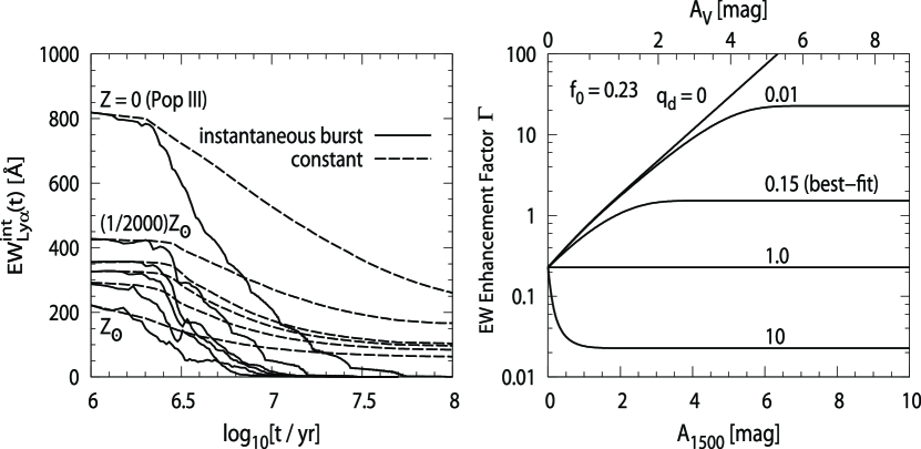
Figure 1.— Left: the time evolution of $\mathrm{EW_{Ly\alpha}^{int}}$ (“intrinsic” Ly$\alpha$ EW determined by stellar spectra and the case B recombination with the assumption all of LyC photons are absorbed and reprocessed into Ly$\alpha$ photons in H II regions) assuming the S03 population synthesis model with the Salpeter IMF. The solid and dashed curves represent the $\mathrm{EW_{Ly\alpha}^{int}}$ evolution for instantaneous starburst and constant star formation, respectively. Several curves are shown corresponding to different stellar metallicities: $Z/Z_{\odot}=0$, $1/2000$, $1/50$, $1/20$, $1/5$, and $1$, from top to bottom. Right: the EW enhancement factor $\Gamma$ as a function of the extinction magnitude at 1500 Å, $A_{1500}$, or at V-band, $A_{V}$. We plot $\Gamma$ for several values of $q_{d}$ (including the value of $q_{d}=0.15$ used in our LAE model) in the range of $q_{d}=0-10$ as indicated in the figure, while $f_{0}$ is fixed to $0.23$ (the value used in the model).

Figure 2.— Cumulative LAE Ly$\alpha$ LFs at $z\sim 3$–6. The model predictions are represented by the curves, while the observational data are plotted by the filled symbols with error-bars. At each panel, the model LAEs are selected with the same threshold value of $\mathrm{EW_{Ly\alpha}^{th}}$ as that adopted in each observation, which is indicated in each panel. The vertical dashed line in each panel is the threshold value of $L_{\mathrm{Ly\alpha}}^{\mathrm{th}}$ of each observation. Top: the predictions from three different $f_{\mathrm{esc}}^{\mathrm{Ly\alpha}}$ model are shown; the simply proportional, the outflow$+$dust (screen), and the outflow$+$dust (slab) models are represented by the dotted, dashed, and solid curves, respectively. Bottom: the contributions from quiescent, pre-outflow phase starburst, and outflow phase starburst are plotted separately by the dotted, short-dashed, and long-dashed curves, respectively, in the outflow$+$dust (slab) model. The references for data points are Shimasaku et al. (2006), Gronwall et al. (2007), and Ouchi et al. (2008). The arrows are taken from Ouchi et al. (2008) which represent the Ly$\alpha$ luminosity range where Ly$\alpha$ LFs are dominated by LAEs with AGN activities.

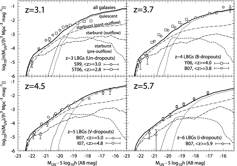
Figure 3.— Rest-frame UV ($\lambda=1500$ Å) LFs of all (i.e., including non-LAEs) galaxies at $z\sim 3$–6. The curves are predictions by our model, while the open symbols with error-bars are the observed data of the LBGs at similar redshifts. The contributions from the quiescent galaxies and the starbursts in the pre-outflow, outflow, and post-outflow phases are shown separately by the dotted, short-dashed, long-dashed, and dash-dotted curves, respectively. Note that post-outflow galaxies are assumed to produce no Ly$\alpha$ photon and hence do not contribute to the model LAE population, but contribute to LBGs by UV continuum (see text). The references for the data points of LBGs are Steidel et al. (1999), Sawicki & Thompson (2006), Yoshida et al. (2006), Bouwens et al. (2007), and Iwata et al. (2007).

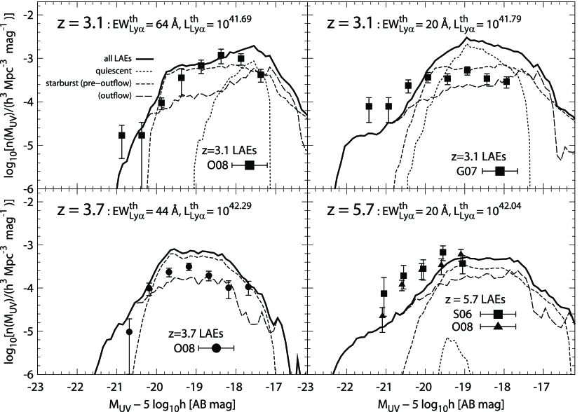
Figure 4.— The same as Fig. 3 but for LAE UV LFs. The curves are the model predictions, while the solid symbols with error-bars are the observed data of the LAEs. The model LAEs have been selected with the same values of $L_{\mathrm{Ly\alpha}}^{\mathrm{th}}$ and $\mathrm{EW_{Ly\alpha}^{th}}$ with those adopted in each observation shown in each panel (the unit of $L_{\mathrm{Ly\alpha}}^{\mathrm{th}}$ is $h^{-2}\ \mathrm{ergs\ s^{-1}}$). Both of the top panels are the UV LFs of the LAEs at $z=3.1$, but they are selected with different criteria. The line markings are the same as Fig. 3. The references for the data points of LAEs are Shimasaku et al. (2006), Gronwall et al. (2007), and Ouchi et al. (2008).

Figure 5.— Rest-frame EW distributions for LAEs at $z\sim 3$–6. The curves are predictions by our model, while the histograms are the observations. The observed data based on spectroscopically confirmed LAEs are labeled as “spec”, while those based on photometric samples as “phot”. The error bars and upper limits are the $1\sigma$ Poissonian statistics for small sample number (Gehrels 1986). The line markings of the model curves are the same as Fig. 3. The vertical dashed line indicates the maximum $\mathrm{EW_{Ly\alpha}^{int}}$ value (240 Å) powered by star-formation activity with the Salpeter IMF and the solar metallicity (Charlot & Fall 1993; Schaerer 2003). The references of the data are given in Fig. 4, except for Dawson et al. (2007).

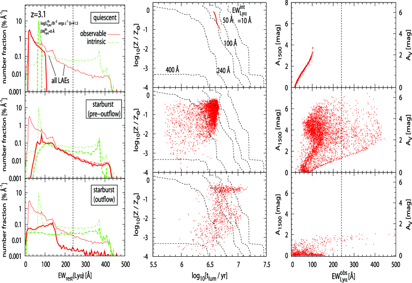
Figure 6.— The left, middle, and right panels show EW distributions (intrinsic and observable), luminosity-weighted age ($t_{\rm lum}$) versus metallicity, and observable EW versus extinction, respectively, of the model LAEs at $z=3.1$. The quantity $t_{\rm lum}$ represents a typical age of stellar population that is responsible for Ly$\alpha$ EW (see text for exact definition). The contributions from quiescent, pre-outflow phase starburst, and outflow phase starburst are shown separately from top to bottom panels. In the left panels, total EW distributions including all of the three populations (quiescent, pre-outflow, and outflow) are also shown by thin curves. The small dots in the middle and right panels are model galaxies. In the middle column, the contours of $\mathrm{EW_{Ly\alpha}^{int}}$ of instantaneous starburst population (shown in Fig. 1) are shown. The model LAEs are selected with $\mbox{$L_{\mathrm{Ly\alpha}}^{\mathrm{th}}$}=10^{41.5}\ h^{-2}\ \mathrm{ergs\ s^{-1}}$, but with no selection about $\mathrm{EW_{\rm Ly\alpha}}$.

Figure 7.— $A_{1500}$ (left ordinate) or $A_{V}$ (right ordinate) versus $\mathrm{EW_{\rm Ly\alpha}}$. The distribution of model LAEs at $z=4.5$ are represented by small dots in the top panel. The selection criteria of model LAEs are indicated in the top panel, which are identical to those adopted in Finkelstein et al. (2009a). In the middle and bottom panels, the median of the model LAE distribution is shown by the filled circles connected by solid lines, while the $10-90$ percentiles are represented by the gray regions. The open symbols with error-bars are observational data of 14 LAEs at $z\sim 4.5$ given by Finkelstein et al. (2009a). The data of $A_{1500}$ were derived by their SED fittings and its typical error is $\sim 0.8$ mag (S. Finkelstein, private communication). The $\mathrm{EW_{\rm Ly\alpha}}$ data in the middle panel were derived by direct observational measurements, while those in the bottom panel were estimated by their SED fittings. The open squares and circles represent the best-fit values using the single population model and two-burst model, respectively, in their SED fittings.

Figure 8.— Distributions of LAEs in the $M_{\rm UV}$-$\mathrm{EW_{\rm Ly\alpha}}$ plane at $z\sim$3–6. In the upper panels, model LAEs are plotted by small dots. In the lower panels, the open symbols are corresponding to each of the observed galaxies. The filled circles connected by solid lines are the mean of the model galaxies, and the gray region represents the $10-90$ percentiles of the model galaxies. See Fig. 4 for the references. The solid curve and horizontal line in each panel indicate $L_{\mathrm{Ly\alpha}}^{\mathrm{th}}$ and $\mathrm{EW_{Ly\alpha}^{th}}$, respectively. Note that $M_{\rm UV}$ is in the rest-frame 1500 Å, and we must convert it in the rest-frame Ly$\alpha$ wavelength to depict the curve of $L_{\mathrm{Ly\alpha}}^{\mathrm{th}}$. We assumed a SED with $\beta=-2$ as an approximation here. The dotted curves show the contours of Ly$\alpha$ line luminosity corresponding to $2\times 10^{43}$, $10^{43}$, and $5\times 10^{42}\ \mbox{$h^{-2}~{}\mathrm{ergs~{}s^{-1}}$}$ from top left to bottom right, assuming $\beta=-2$.

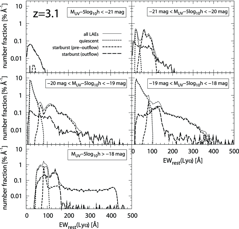
Figure 9.— EW distribution for various $M_{\rm UV}$ intervals at $z=3.1$. Note that $M_{\rm UV}$ is the observable (i.e., extinction uncorrected) one. The selection criteria of model LAEs are $\mbox{$L_{\mathrm{Ly\alpha}}^{\mathrm{th}}$}=10^{41.5}\ h^{-2}\ \mathrm{ergs\ s^{-1}}$ and $\mbox{$\mathrm{EW_{Ly\alpha}^{th}}$}=0$ Å. The line markings are indicated in the upper-left panel (the same as Fig. 3).

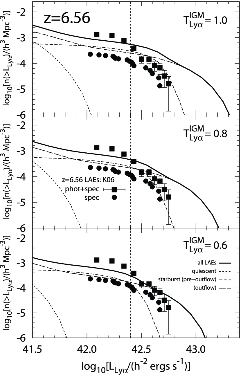
Figure 10.— Comparisons between the cumulative Ly$\alpha$ LF data of Kashikawa et al. (2006) at $z=6.56$ and model predictions with three different values of the IGM transmission for Ly$\alpha$ photons, $\mbox{$T_{\mathrm{Ly\alpha}}^{\mathrm{IGM}}$}=$1.0 (top), 0.8 (middle), and 0.6 (bottom). The thick solid curve is for all model LAEs, and the other curves are for model LAEs with different phases (the same line markings as those of the lower panels of Fig. 2). The filled squares are all LAE candidates in the K06 sample, while the filled circles are those with spectroscopic confirmation. The vertical dashed line indicates the threshold Ly$\alpha$ luminosity of $10^{42.4}\ h^{-2}\ \mathrm{ergs\ s^{-1}}$, which will be applied in the comparisons with UV LF, EW distribution, and $M_{\mathrm{UV}}-\mbox{$\mathrm{EW_{\rm Ly\alpha}}$}$ plane (see Fig. 11).

Figure 11.— The same as Fig. 10, but for comparisons with UV LF, EW distribution, and $M_{\mathrm{UV}}-\mbox{$\mathrm{EW_{\rm Ly\alpha}}$}$ plane from the left to the right panels. The line markings of the model curves in the left, middle, and right panels are the same as those of Figs. 4, 5, and 8, respectively. Here, only LAE candidates having $\mbox{$L_{\mathrm{Ly\alpha}}^{\mathrm{obs}}$}\geq 10^{42.4}\ h^{-2}\ \mathrm{ergs\ s^{-1}}$ are used from the K06 sample, and this condition is included in the model predictions as well. The vertical dotted lines in the UV LF and $M_{\mathrm{UV}}-\mbox{$\mathrm{EW_{\rm Ly\alpha}}$}$ plane indicate the 1 and 2 $\sigma$ limiting UV continuum magnitudes of Kashikawa et al. (2006).

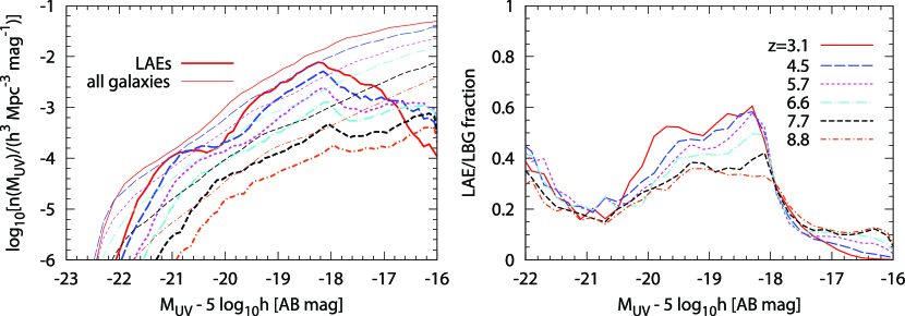
Figure 12.— Redshift evolution of LAE UV LF (left) and LAE fraction in LBGs as a function of UV luminosities (right) predicted by our model from $z=3.1$ to $z=8.8$ with $\mbox{$T_{\mathrm{Ly\alpha}}^{\mathrm{IGM}}$}=1$. The dashed curves in the left panel show the UV LFs of all galaxies (or observationally, LBGs). The galaxies with $\mbox{$L_{\mathrm{Ly\alpha}}^{\mathrm{obs}}$}\geq\mbox{$L_{\mathrm{Ly\alpha}}^{\mathrm{th}}$}=10^{41.5}~{}\mbox{$h^{-2}~{}\mathrm{ergs~{}s^{-1}}$}$ and $\mbox{$\mathrm{EW_{\rm Ly\alpha}}$}\geq\mbox{$\mathrm{EW_{Ly\alpha}^{th}}$}=20$ Å are selected as LAEs regardless of redshift.

Figure 13.— UV LFs of LAEs at $z=3.1$ predicted by our model with different values of threshold $\mathrm{EW_{Ly\alpha}^{th}}$ (left) and $L_{\mathrm{Ly\alpha}}^{\mathrm{th}}$ (right) in LAE selection. The thin solid curve represents the UV LF of all galaxies including non-LAEs. The observed data of UV LFs of LAEs at $z=3.1$ obtained by Gronwall et al. (2007, G07) and Ouchi et al. (2008, O08) are also shown. Their LAE selection thresholds are $[\mbox{$L_{\mathrm{Ly\alpha}}^{\mathrm{th}}$}/(h^{-2}\ {\rm ergs\ s^{-1}}),\ \mbox{$\mathrm{EW_{Ly\alpha}^{th}}$}/\mathrm{\mathring{A}}]=(10^{41.79},\ 20)$ and $(10^{41.69},\ 64)$ for G07 and O08, respectively.

References

- Adelberger & Steidel (2000) Adelberger, K. L., & Steidel, C. C. 2000, ApJ, 544, 218
- Ando et al. (2006) Ando, M., Ohta, K., Iwata, I., Akiyama, M., Aoki, K., & Tamura, N. 2006, ApJ, 645, L9
- Atek et al. (2008) Atek, H., Kunth, D., Hayes, M., Östlin, G., Mas-Hesse, J. M. 2008, A&A, 488, 491
- Baldwin (1977) Baldwin, J. A. 1977, ApJ, 214, 679
- Barton et al. (2004) Barton, E. J., Davé, R., Smith, J.-D. T., Papovich, C., Hernquist, L., & Springel, V. 2004, ApJ, 604, L1
- Bouwens et al. (2007) Bouwens, R. J., Illingworth, G. D., Franx, M., & Ford, H. 2007, ApJ, 670, 928
- Bruzual & Charlot (1993) Bruzual, G. A., & Charlot, S. 1993, ApJ, 405, 538
- Buat, V. et al. (2009) Buat, V., Takeuchi, T. T., Burgarella, D., Giovannnoli, E., Murata, K. L. 2009, preprint (arXiv:0907.2819)
- Charlot & Fall (1993) Charlot, S., & Fall, S. M. 1993, ApJ, 415, 580
- Clemens & Alexander (2004) Clemens, M. S., & Alexander, P. 2004, MNRAS, 350, 66
- Cowie & Hu (1998) Cowie, L. L., & Hu, E. M. 1998, AJ, 115, 1319
- Dawson et al. (2007) Dawson, S. et al. 2007, ApJ, 671, 1227
- Dayal et al. (2008) Dayal, P., Ferrara, A., & Gallerani, S. 2008, MNRAS, 389, 1683
- Dayal et al. (2009) Dayal, P., Ferrara, A., Saro, A., Salvaterra, R., Borgani, S., & Tornatore, L. 2009, preprint (arXiv:0907.0337)
- Deharveng et al. (2008) Deharveng, J.-M. et al. 2008, ApJ, 680, 1072
- Dijkstra et al. (2007a) Dijkstra, M., Lidz, A., & Wyithe, J. S. B. 2007a, MNRAS, 377, 1175
- Dijkstra et al. (2007b) Dijkstra, M., Whyithe, J. S. B., & Haiman, Z. 2007b, MNRAS, 379, 253
- Dijkstra & Wyithe (2007) Dijkstra, M., & Wyithe, J. S. B. 2007, MNRAS, 379, 1589
- Fan et al. (2006) Fan, X., Carilli, C. L., & Keating, B. 2006, ARA&A, 44, 415
- Finkelstein et al. (2008) Finkelstein, S. L., Rhoads, J. E., Malhotra, S., Grogin, N., & Wan, J. 2008, ApJ, 678, 655
- Finkelstein et al. (2009a) Finkelstein, S. L., Rhoads, J. E., Malhotra, S., & Grogin, N. 2009a, ApJ, 691, 465
- Finkelstein et al. (2009b) Finkelstein, S. L., Cohen, S. H., Malhotra, S., & Rhoads, J. E. 2009b, ApJ, 700, 276
- Gawiser et al. (2006) Gawiser, E. et al. 2006, ApJ, 642, L13
- Gronwall et al. (2007) Gronwall, C. et al. 2007, ApJ, 667, 79
- Haiman & Cen (2005) Haiman, Z., & Cen, R. 2005, ApJ, 623, 627
- Hansen & Oh (2006) Hansen, M., & Oh, S. P. 2006, MNRAS, 367, 979
- Hu et al. (2004) Hu, E. M., Cowie, L. L., Capak, P., McMahon, R. G., Hayashino, T., & Komiyama, Y. 2004, AJ, 127, 563
- Inoue et al. (2006) Inoue, A., Iwata, I., & Deharveng, J.-M. 2006, MNRAS, 371, L1
- Iwata et al. (2007) Iwata, I., Ohta, K., Tamura, N., Akiyama, M., Aoki, K., Ando, M., Kiuchi, G., & Sawicki, M. 2007, MNRAS, 376, 1557
- Iye et al. (2006) Iye, M. et al. 2006, Nature, 443, 186
- Kashikawa et al. (2006) Kashikawa, N. et al. 2006, ApJ, 648, 7
- Kobayashi et al. (2007) Kobayashi, A. R. M., Totani, T., & Nagashima, M. 2007, ApJ, 670, 919 (KTN07)
- Le Delliou et al. (2006) Le Delliou, M., Lacey, C. G., Baugh, C. M., & Morris, S. L. 2006, MNRAS, 365, 712
- Leitherer et al. (1999) Leitherer, C. et al. 1999, ApJS, 123, 3
- Madau (1995) Madau, P. 1995, ApJ, 441, 18
- Malhotra & Rhoads (2002) Malhotra, S., & Rhoads, J. E. 2002, ApJ, 565, L71
- Malhotra & Rhoads (2004) Malhotra, S., & Rhoads, J. E. 2004, ApJ, 617, L5
- Mao et al. (2007) Mao, J., Lapi, A., Granato, G. L., de Zotti, G., & Danese, L. 2007, ApJ, 667, 655
- Mesinger & Furlanetto (2008) Mesinger, A., & Furlanetto, S. R. 2008, MNRAS, 386, 1990
- Murayama et al. (2007) Murayama, T. et al. 2007, ApJS, 172, 523
- Nagamine et al. (2008) Nagamine, K., Ouchi, M., Springel, V., & Hernquist, L. 2008, preprint (arXiv:0802.0228)
- Nagashima & Yoshii (2004) Nagashima, M., & Yoshii, Y. 2004, ApJ, 610, 23
- Nagashima et al. (2005) Nagashima, M., Yahagi, H., Enoki, M., Yoshii, Y., & Gouda, N. 2005, ApJ, 634, 26
- Neufeld (1991) Neufeld, D. A. 1991, ApJ, 370, L85
- Orsi et al. (2008) Orsi, A., Lacey, C. G., Baugh, C. M., & Infante, L. 2008, MNRAS, 391, 1589
- Östlin et al. (2009) Östlin, G., Hayes, M., Kunth, D., Mas-Hesse, J. M., Leitherer, C., Petrosian, A. & Atek, H. 2009, ApJ, 138, 923
- Ota et al. (2008) Ota, K. et al. 2008, ApJ, 677, 12
- Ouchi et al. (2008) Ouchi, M. et al. 2008, ApJS, 176, 301
- Pei (1992) Pei, Y. C. 1992, ApJ, 395, 130
- Pentericci et al. (2009) Pentericci, L., Grazian, A., Fontana, A., Castellano, M., Giallongo, E., Salimbeni, S., & Santini, P. 2009, A&A, 494, 553
- Reddy et al. (2008) Reddy, N. A., Steidel, C. C., Pettini, M., Adelberger, K. L., Shapley, A. E., Erb, D. K., & Dickinson, M. 2008, ApJS, 175, 48
- Rhoads et al. (2000) Rhoads, J. E., Malhotra, S., Dey, A., Stern, D., Spinrad, H., & Jannuzi, B. T. 2000, ApJ, 545, L85
- Rybicki & Lightman (1979) Rybicki, G. B., & Lightman, A. P. 1979, Radiative Processes in Astrophysics (New York: Wiley)
- Samui (2009) Samui, S., Srianand, R., & Subramanian, K. 2009, MNRAS, 398, 2061
- Santos (2004) Santos, M. R. 2004, MNRAS, 349, 1137
- Sawicki & Thompson (2006) Sawicki, M., & Thompson, D. 2006, ApJ, 642, 653
- Schaerer (2003) Schaerer, D. 2003, A&A, 397, 527 (S03)
- Schaerer & Verhamme (2008) Schaerer, D., & Verhamme, A. 2008, A&A, 480, 369
- Shapley et al. (2003) Shapley, A. E., Steidel, C. C., Pettini, M., and Adelberger, K. L. 2003, ApJ, 588, 65
- Shimasaku et al. (2006) Shimasaku, K. et al. 2006, PASJ, 58, 313
- Shioya et al. (2009) Shioya, Y. et al. 2009, ApJ, 696, 546
- Stanway et al. (2007) Stanway, E. R. et al. 2007, MNRAS, 376, 727
- Steidel et al. (1999) Steidel, C. C., Adelberger, K. L., Giavalisco, M., Dickinson, M., & Pettini, M., 1999, ApJ, 519, 1
- Taniguchi et al. (2005) Taniguchi, Y. et al. 2005, PASJ, 57, 165
- Verhamme et al. (2008) Verhamme, A., Schaerer, D., Atek, H., & Tapken, C. 2008, A&A, 491, 89
- Yoshida et al. (2006) Yoshida, M. et al. 2006, ApJ, 653, 988
- Yoshii & Peterson (1994) Yoshii, Y., & Peterson, B. A. 1994, ApJ, 1994, 436, 551