KIAS-P09009

Nonrelativistic Superconformal M2-Brane Theory

Ki-Myeong Lee^†, Sangmin Lee^‡, Sungjay Lee^†

^†Korea Institute for Advanced Study, Seoul 130-722, Korea
^‡Department of Physics, Seoul National University, Seoul 151-747, Korea

We investigate the low energy physics of particles in the symmetric phase of the ${\cal N}=6$ mass-deformed ABJM theory in terms of the superconformal nonrelativistic field theory with 14 supercharges. They describe a certain kind of excitations on M2 branes in the background of external four-form flux. We study the nonrelativistic superconformal algebra and their representations by using the operator-state correspondence with the related harmonic oscillator Hamiltonian. We find the unitarity bounds on the scaling dimension and particle number of any local operator, and comment on subtleties in computing the superconformal Witten index that counts the chiral operators.

1 Introduction and Concluding Remarks

Recently there have been much interests in the construction of gravity dual for the nonrelativistic conformal theories  [1, 2, 3, 4, 5, 6, 7]. The nonrelativistic conformal symmetry, so-called the Schrödinger symmetry [8, 9], has appeared in many condensed matter systems, and also in some class of nonrelativistic field theories [10].

In last year, Aharony, Bergman, Jafferis, and Maldacena (ABJM) have proposed a three-dimensional superconformal Chern-Simons matter theory as a theory on multiple M2 branes in an orbifold $\mathbb{C}^{4}/Z_{k}$ [11]. This ABJM model has ${\cal N}=6$ supersymmetries and $SU(4)_{R}\times U(1)$ global symmetries. This theory has a mass-deformation which preserves supersymmetry but reduces $SU(4)_{R}$ symmetry to $SU(2)\times SU(2)\times U(1)$ and breaks conformal symmetry [12, 13, 14]. While this deformed theory has discrete vacua [14], its nonrelativistic limit in the symmetric phase turns out to acquire a superconformal symmetry which is different from the original mass-deformed ABJM model.

In this work, we investigate in details the nonrelativistic superconformal ABJM model. We write down the theory, which is characterized by the mass parameter $m$, gauge group $U(N)\times U(N)$, and the Chern-Simons level $k$. We also find its symmetries and conserved charges, and study the symmetry algebra and its representations. This nonrelativistic theory describes the low energy dynamics of a number of massive charged particles, not a mixed set of particles and anti-particles, in the symmetric phase of the relativistic mass-deformed ABJM model. In addition to the conformal symmetry, the number of supercharges also increases from the original 12 to 14. These 14 supercharges get split to 10 kinematical supercharges, 2 dynamical supercharges and 2 conformal supercharges. We study the representations of the nonrelativistic superconformal (super Schrödinger) algebra in the related many-body theory with a harmonic potential. There are interesting bounds on the scaling dimension $\Delta_{\cal O}$ and the particle number $N_{\cal O}$ of a local operator ${\cal O}$ by its charges. We also comment on the superconformal Witten index which counts the so-called chiral operators.

In the symmetric phase of the mass-deformed ABJM model, there is no massless particles in the symmetric phase and so a pair of particle and antiparticle cannot annihilate to the vacuum and would remain as a sort of massive meson state with maybe some bound energy. Thus one has to decide whether one wants to keep only particles or both particles and anti-particles in the nonrelativistic limit, which changes the nonrelativistic theory and its supersymmetries. In our case, the ABJM model has the global $U(1)$ symmetry to start with, and so we keep only particles of positive $U(1)$ charge in the low energy dynamics. If we have kept both particles and antiparticles in the nonrelativistivic dynamics, all 12 supersymmetries would become kinematical and there would be no additional conformal supercharges.

Similar question would arise in the study of the nonrelativistic limit of the related ${\cal N}=8$ Bagger-Lambert-Gustavsson (BLG) model  [15, 16, 17, 18, 19]. The BLG model also has the supersymmetry preserving mass deformation which breaks $SO(8)$ R-symmetry to $SO(4)\times SO(4)$ R-symmetry, which allows the nonrelativistic limit in the symmetric phase [20, 21]. As there are no $U(1)$ symmetry in the BLG model, we do not have a predetermined notion of particles and antiparticles as in the ABJM model. The straightforward nonrelativistic limit of the BLG model, which keeps all kinds of massive particles, lead to only kinematical supercharges. Instead, if we keep particles in the sense of the ABJM model, then we end up with precisely the same symmetry algebra as in the ABJM model.

It is well-known that the theories with the $d$-dimensional Schrödinger symmetry can be obtained by performing the discrete light-cone quantization (DLCQ) of theories with the $(d+1)$-dimensional relativistic conformal symmetry. As pointed out in [4], the DLCQ of field theories however raises many subtle issues, and as a consequence it seems rather difficult to obtain the explicit field theory Lagrangians. Recent works [1, 2, 3, 4, 5, 6, 7] to construct the supergravity solutions of interest rely on the DLCQ embedding, so their interpretation in terms of the dual field theories remains unclear.

Since our work begins with the ABJM model with a definite proposal for the gravity dual, our work may help to build the first concrete example of nonrelativistic holography. The gravity dual of the ABJM model is $AdS_{4}\times S^{7}/Z_{k}$, and the mass deformation can be induced by introducing a certain class of four-form field strength to this geometry [22, 23]. Now we want to keep only particles in the symmetric phase. How we can manage this in its gravitational counter part is not clear at the moment.

In the relativistic conformal field theories, there has been a natural correspondence between operators and states by considering the theory on spheres instead of plane. This can be achieved by the radial quantization of the Euclidean time theory as space and time has the same scaling dimension. This leads to a simple representation of the conformal symmetry algebras. Since the nonrelativistic conformal theories has anisotropic scaling behaviors of time and space $(t,x_{i})\rightarrow(\lambda^{2}t,\lambda x_{i})$, one can not simply apply the above idea in our nonrelativistic ABJM model. However, the recent work by Nishida and Son [10] has shown that one can define a new Hamiltonian with a harmonic potential for a given theory with Schrödinger symmetry and find the energy eigenvalues and states of the system with the harmonic potential for a given conformal primary operators. We generalize this scheme of the operator-state correspondence to our supersymmetric case and get some useful unitarity bound on scaling dimension and particle number of any given operator in terms of its other quantum numbers. The so-called chiral operator saturates the bound of the scaling dimension.

The key challenge of our nonrelativistic superconformal field theory with nonabelian gauge group $U(N)\times U(N)$ would be how to impose the local Gauss law and how to find the gauge-invariant operators. From the nature of the Gauss law, one can see the elementary physical fields should carry both charge and magnetic flux of the abelian $U(1)\times U(1)$. In addition, one should impose the non-abelian Gauss law to get a charge-flux composite operators. While they would be invariant under the local nonabelian gauge transformations, we expect that they would form also nontrivial representations of the global part of $U(N)\times U(N)$ gauge symmetry. As charge-flux composite operators, the physical operators would be also quasi-local. The correlation functions of these operators and their operator products would be of much physical interest. It would be interesting to calculate their scaling dimensions and correlation functions perturbatively in the weak coupling limit.

We argue that the resulting charge-flux operators as the gauge invariant creation and annihilation operators for each massive particles are chiral operators at least in the weak coupling limit. Maybe only certain kind of operator products of these flux-charge composite operators would remain chiral. One can define the Witten index to count the chiral operators, and these would contribute to the counting. This contradicts with the definition of the chiral operators in the relativistic theory where they should be gauge singlet or invariant. Any physical operators or states of the nonrelativistic theory also needs to be invariant under the local gauge transformation, but this does not mean that, as the flux-charge composite objects, they have to be singlet under the global part of the gauge transformation.

There has been many studies of the massive Chern-Simons-matter theories of less supersymmetries and their nonrelativistic counter parts [24], and further of the superconformal theory [25]. Also a further investigation of super-Schrödinger algebra has been also studied in Ref. [26, 27, 28] More recently there has been a series of work by Nakayama et al on the subject [29, 30]. This study has led to two classes of nonrelativistic supercharges: kinematical ones and dynamical ones. Moreover these nonrelativistic theories has the BPS soliton spectrum [31], defined by the covariantly holomorphic matter fields satisfying the Gauss law. In our nonrelativistic model, one see that similar solitons, if exist, would be classical versions of chiral or anti-chiral operators.

The contents of the paper are organized as follows. In Sec. 2, we take the nonrelativistic limit of the ABJM model. In Sec. 3, we find many symmetries and the corresponding charges, including supersymmetries and nonrelativistic superconformal symmetries. In Sec. 4, we explore the representation of the superalgebra and study chiral primary operators with some unitarity bounds on scaling dimensions.

Note added: While we were preparing this paper, a preprint appeared on the arXiv which contains some overlap with our work [44].

2 Nonrelativistic Limit of the Mass-deformed ABJM Model

2.1 The mass-deformed ABJM model

Let us start with a short description on the ABJM model [11], believed to describe the dynamics of multiple M2-branes probing a certain orbifold geometry. This ${\cal N}=6$ supersymmetric model has the gauge symmetry $G=U(N)_{k}\times U(N)_{-k}$ whose gauge fields are denoted by $A_{\mu}$ and $\tilde{A}_{\mu}$ with the Chern-Simons kinetic term of level $(k,-k)$. The bi-fundamental matter fields are composed of four complex scalars $Z_{\alpha}$ ($\alpha=1,2,3,4$) and four three-dimensional spinors $\Psi^{\alpha}$, both of which transform under the gauge symmetry as $({\bf N},\bar{\bf N})$. As well as the gauge symmetry, the present model also has additional global $SU(4)_{R}\times U(1)$ symmetry, under which the scalars $Z_{\alpha}$ furnish the representation ${\bf 4}_{+}$ while the fermions $\Psi^{\alpha}$ furnish ${\bf\bar{4}}_{+}$.

For the clarity we hereafter reintroduce the Planck constant $\hbar$ and speed of light $c$ in our discussions. The ABJM Lagrangian is made of several parts

$${\cal L}={\cal L}_{\text{CS}}+{\cal L}_{\text{kin}}+{\cal L}_{\text{Yukawa}}+{\cal L}_{\text{potential}}\ ,$$ (2.1)

the Chern-Simons and kinetic terms

$${\cal L}_{\text{CS}}+{\cal L}_{\text{kin}} = \frac{k\hbar c}{4\pi}\epsilon^{\mu\nu\rho}\text{Tr}\Big{(}A_{\mu}\partial_{\nu}A_{\rho}-\frac{2i}{3}A_{\mu}A_{\nu}A_{\rho}-\tilde{A}_{\mu}\partial_{\nu}\tilde{A}_{\rho}+\frac{2i}{3}\tilde{A}_{\mu}\tilde{A}_{\nu}\tilde{A}_{\rho}\Big{)}$$ (2.2)

$$\hskip 8.5359pt-\text{Tr}\left(D_{\mu}\bar{Z}^{\alpha}D^{\mu}Z_{\alpha}+i\bar{\Psi}_{\alpha}\gamma^{\mu}D_{\mu}\Psi^{\alpha}\right)\ ,$$

the Yukawa-like interactions

$${\cal L}_{\text{Yukawa}} = \frac{2\pi i}{k\hbar c}\text{Tr}\Big{(}\bar{Z}^{\alpha}Z_{\alpha}\bar{\Psi}_{\beta}\Psi^{\beta}-Z_{\alpha}\bar{Z}^{\alpha}\Psi^{\beta}\bar{\Psi}_{\beta}+2Z_{\alpha}\bar{Z}^{\beta}\Psi^{\alpha}\bar{\Psi}_{\beta}-2\bar{Z}^{\alpha}Z_{\beta}\bar{\Psi}_{\alpha}\Psi^{\beta}$$ (2.3)

$$\hskip 36.98866pt+\epsilon_{\alpha\beta\gamma\delta}\bar{Z}^{\alpha}\Psi^{\beta}\bar{Z}^{\gamma}\Psi^{\delta}-\epsilon^{\alpha\beta\gamma\delta}Z_{\alpha}\bar{\Psi}_{\beta}Z_{\gamma}\bar{\Psi}_{\delta}\Big{)}\ ,$$

and the sextic scalar interactions

$${\cal L}_{\text{potential}} = -\frac{4\pi^{2}}{3k^{2}\hbar^{2}c^{2}}\text{Tr}\Big{(}6Z_{\alpha}\bar{Z}^{\alpha}Z_{\beta}\bar{Z}^{\gamma}Z_{\gamma}\bar{Z}^{\gamma}-4Z_{\alpha}\bar{Z}^{\beta}Z_{\gamma}\bar{Z}^{\alpha}Z_{\beta}\bar{Z}^{\gamma}$$ (2.4)

$$\hskip 54.06006pt-Z_{\alpha}\bar{Z}^{\alpha}Z_{\beta}\bar{Z}^{\beta}Z_{\gamma}\bar{Z}^{\gamma}-Z_{\alpha}\bar{Z}^{\beta}Z_{\beta}\bar{Z}^{\gamma}Z_{\gamma}\bar{Z}_{a}\Big{)}\ .$$

The positive definite potential ${\cal V}_{0}$ can be expressed in terms of third order polynomials $W$ and their hermitian conjugates $\bar{W}$:

$${\cal V}=\frac{2}{3}\text{Tr}\Big{(}W^{\alpha}_{\beta\gamma}\bar{W}^{\beta\gamma}_{\alpha}\Big{)}$$ (2.5)

with

$$W_{\beta\gamma}^{\alpha}=-\frac{\pi}{k\hbar c}\Big{(}2Z_{\beta}\bar{Z}^{\alpha}Z_{\gamma}+\delta^{\alpha}_{\beta}(Z_{\gamma}\bar{Z}^{\rho}Z_{\rho}-Z_{\rho}\bar{Z}^{\rho}Z_{\gamma})\Big{)}-(\beta\ \leftrightarrow\ \gamma)\ ,$$

$$\bar{W}^{\beta\gamma}_{\alpha}=+\frac{\pi}{k\hbar c}\Big{(}2\bar{Z}^{\beta}Z_{\alpha}\bar{Z}^{\gamma}+\delta_{\alpha}^{\beta}(\bar{Z}^{\gamma}Z_{\rho}\bar{Z}^{\rho}-\bar{Z}^{\rho}Z_{\rho}\bar{Z}^{\gamma})\Big{)}-(\beta\ \leftrightarrow\ \gamma)\ .$$ (2.6)

We basically use the convention of [13] except the hermitian gauge fields so that the covariant derivatives now become

$$D_{\mu}Z_{\alpha}=\partial_{\mu}Z_{\alpha}-iA_{\mu}Z_{\alpha}+iZ_{\alpha}\tilde{A}_{\mu},$$ (2.7)

and the explicit c dependence in temporal Lorentz indices, for examples, $\partial_{0}=\partial_{t}/c$. It is known that this theory is invariant under the $\mathbb{Z}_{2}$ symmetry, or parity $Z_{\alpha},\Psi^{\alpha},A_{\mu},\tilde{A}_{\mu}\leftrightarrow\bar{Z}^{\alpha},\bar{\Psi}_{\alpha},\tilde{A}_{\mu},A_{\mu}$. For the gauge invariance, the Chern-Simons level $k$ is required to be integer quantized, and is chosen to be positive $k>0$ in this paper. The trace is over $N\times N$ matrices of either gauge group and leaves the gauge invariant quantities. The spinor contraction is the standard one.

This Lagrangian is invariant under the ${\cal N}=6$ supersymmetry whose transformation rules are

$$\delta Z_{\alpha} = i\xi_{\alpha\beta}\Psi^{\beta},$$

$$\delta\bar{Z}^{\alpha} = i\xi^{\alpha\beta}\bar{\Psi}_{\beta},$$

$$\delta\Psi^{\alpha} = -\gamma^{\mu}\xi^{\alpha\beta}D_{\mu}Z_{\beta}+W^{\alpha}_{\beta\gamma}\xi^{\beta\gamma},$$

$$\delta\bar{\Psi}_{\alpha} = -\gamma^{\mu}\xi_{\alpha\beta}D_{\mu}\bar{Z}^{\beta}+\bar{W}^{\beta\gamma}_{\alpha}\xi_{\beta\gamma},$$

$$\delta A_{\mu} = +\frac{2\pi}{k\hbar c}(Z_{\alpha}\bar{\Psi}_{\beta}\gamma_{\mu}\xi^{\alpha\beta}+\Psi^{\alpha}\bar{Z}^{\beta}\gamma_{\mu}\xi_{\alpha\beta}),$$

$$\delta\tilde{A}_{\mu} = -\frac{2\pi}{k\hbar c}(\bar{\Psi}_{\alpha}Z_{\beta}\gamma_{\mu}\xi^{\alpha\beta}+\bar{Z}^{\alpha}\Psi^{\beta}\gamma_{\mu}\xi_{\alpha\beta})\ .$$ (2.8)

Here the supersymmetry transformation parameters $\xi^{\alpha\beta}=-\xi^{\beta\alpha}$ satisfy the relations

$$\xi_{\alpha\beta}=(\xi^{\alpha\beta})^{*}=\frac{1}{2}\epsilon_{\alpha\beta\gamma\delta}\xi^{\gamma\delta}\ ,$$ (2.9)

with $\epsilon_{1234}=\epsilon^{1234}=1$.

It is well-known that the M2-brane theory allows a mass deformation [12, 13, 14] which preserves whole Poincaré supersymmetry. The mass contribution to the Lagrangian is

$${\cal L}_{\text{m}}=-\text{Tr}\Big{(}M^{\alpha}_{\ \gamma}M^{\gamma}_{\beta}\bar{Z}^{\beta}Z_{\alpha}+i\bar{\Psi}_{\alpha}M^{\alpha}_{\ \beta}\Psi^{\beta}\Big{)}-\frac{4\pi}{k\hbar c}\text{Tr}\Big{(}Z_{a}\bar{Z}^{\alpha}Z_{\beta}\bar{Z}^{\gamma}M^{\beta}_{\ \gamma}-\bar{Z}^{\alpha}Z_{\alpha}\bar{Z}^{\beta}Z_{\gamma}M^{\gamma}_{\ \beta}\Big{)},$$ (2.10)

where the matrix $M^{\alpha}_{\ \beta}$ satisfies

$$M^{\dagger}=M,\qquad\text{Tr}M=0,\qquad M^{2}=\left(\frac{mc}{\hbar}\right)^{2}{\bf 1}_{2}\ .$$ (2.11)

Up to $SU(4)_{R}$ rotation, one can choose $M$ to be diagonal

$$M=\frac{mc}{\hbar}~{}\text{diag}\big{(}1,1,-1,-1\big{)}\ ,$$ (2.12)

which implies that deformation breaks the R-symmetry group down to $SU(2)\times SU(2)\times U(1)$. The mass-deformed ABJM can be understood as the deformation of W tensor as

$$\delta_{\text{m}}W^{\alpha}_{\beta\gamma}=\frac{1}{2}\big{(}M^{\alpha}_{\ \beta}Z_{\gamma}-M^{\alpha}_{\ \gamma}Z_{\beta}\big{)}\ ,\qquad\delta_{m}\bar{W}^{\beta\gamma}_{\alpha}=\frac{1}{2}\big{(}M^{\beta}_{\ \alpha}\bar{Z}^{\gamma}-M^{\gamma}_{\ \alpha}\bar{Z}^{\beta}\big{)}.$$ (2.13)

The total scalar potential, sum of ${\cal V}_{0}$ and the bosonic part of ${\cal L}_{\text{m}}$, can be nicely expressed as complete squares again

$${\cal V}_{\text{total}}=\frac{2}{3}\text{Tr}\Big{[}(W+\delta_{m}W)^{\alpha}_{\beta\gamma}(\bar{W}+\delta_{m}\bar{W})^{\beta\gamma}_{\alpha}\Big{]}\ .$$ (2.14)

This mass-deformed Lagrangian still preserves ${\cal N}=6$ supersymmetry, once the fermionic transformation rules (2.8) are modified as

$$\delta_{m}\Psi^{\alpha}=\delta_{m}W^{\alpha}_{\beta\gamma}\xi^{\beta\gamma},\ \delta_{m}\bar{\Psi}_{\alpha}=\delta_{m}W^{\beta\gamma}_{\alpha}\xi_{\beta\gamma}\ .$$ (2.15)

2.2 A nonrelativistic limit

The mass-deformed potential for the theory with gauge group $U(N)\times U(N)$ has a discrete set of vacua where the scalar fields takes nonzero expectation values with different symmetry breaking patterns [14]. Here we are interested in the symmetric vacuum where the scalar expectation values vanish and there is no broken gauge or global symmetries. In the symmetric vacuum, there are only massive charged particles and antiparticles. One may not expect particle-antiparticle annihilations to massless particles, even though it is not clear at this moment whether they form any stable bound states. For a given number of particles and antiparticles, we can consider the low energy physics where the speed of particles are much slower than that of the speed of light. There would be no particle or antiparticle creations from the collisions as the particle momenta are much smaller than their mass.

There can be many possible nonrelativistic systems obtained from the ABJM model as one can choose what kinds of particles we want to keep in the nonrelativistic theory. Thus, the remaining symmetry including the supersymmetry after the nonrelativistic limit will depends on our choice of particles. For the ABJM model, there is a natural global $U(1)$ symmetry under which all fields $Z_{\alpha},\Psi^{\beta}$ carry the same charge and here we are interested in keeping only particles once we identify the particle number as this global $U(1)$ charge.

As we are looking at the low energy dynamics in the symmetric phase, let us begin by the scalar Lagrangian, ignoring the higher-order interaction terms for a while

$${\cal L}_{\text{scalar}}=\frac{1}{c^{2}}D_{t}\bar{Z}^{\alpha}D_{t}Z_{\alpha}-D_{i}\bar{Z}^{\alpha}D_{i}Z_{\alpha}-\frac{m^{2}c^{2}}{\hbar^{2}}\bar{Z}^{\alpha}Z_{\alpha}\ .$$ (2.16)

Considering the particle modes in the scalar fields

$$Z_{\alpha}=\frac{\hbar}{\sqrt{2m}}\ z_{\alpha}e^{-imc^{2}t/\hbar}\ ,$$ (2.17)

the above Lagrangian in the nonrelativistic limit $c\to\infty$ becomes

$${\cal L}_{\text{scalar}}^{\text{NR}}=\bar{z}^{\alpha}\Big{(}i\hbar D_{t}+\frac{\hbar^{2}}{2m}D_{i}^{2}\Big{)}z_{\alpha}\ ,$$ (2.18)

where $A_{t}=cA_{0}$ is kept finite. The correction term $\sim\hbar^{2}|\partial_{t}z_{\alpha}|^{2}/mc^{2}$ is smaller than the above Lagrangian by the factor $\big{(}p/mc\big{)}^{2}$. As will be explained later, there would be in addition non-vanishing contributions from the quartic interaction terms. The Chern-Simons term in the nonrelativistic limit becomes

$${\cal L}_{\text{CS}}=\frac{k\hbar}{4\pi}\epsilon^{\mu\nu\rho}\text{Tr}\big{(}A_{\mu}\partial_{\nu}A_{\rho}-\frac{2i}{3}A_{\mu}A_{\nu}A_{\rho}-\tilde{A}_{\mu}\partial_{\nu}\tilde{A}_{\rho}+\frac{2i}{3}\tilde{A}_{\mu}\tilde{A}_{\nu}\tilde{A}_{\rho}\big{)},$$ (2.19)

where $\mu,\nu,\rho$ runs $t,x^{1},x^{2}$ instead of $x^{0}=ct,x^{1},x^{2}$.

For the fermionic part of the Lagrangian without the Yukawa interaction

$${\cal L}_{\text{fermion}} = -i\bar{\Psi}\gamma^{\mu}D_{\mu}\Psi\mp\frac{imc}{\hbar}\bar{\Psi}\Psi$$ (2.20)

$$= -i\Psi^{\dagger}\gamma^{0}\Big{(}\frac{1}{c}\gamma^{0}D_{t}+\gamma^{i}D_{i}\Psi\pm\frac{mc}{\hbar}\Big{)}\Psi\ ,$$

it needs a little more elaboration to take the nonrelativistic limit. The upper sign for the mass is for $\Psi^{1},\Psi^{2}$ and the lower sign for $\Psi^{3},\Psi^{4}$. We choose the three-dimensional gamma matrices to be

$$\gamma^{0}=i\tau^{2}\ ,\qquad\gamma^{1}=\tau^{1}\ ,\qquad\gamma^{2}=\tau^{3}\ ,\qquad\gamma^{012}=1\ .$$ (2.21)

Keeping only the particles again, one can expand the fermion fields as

$$\Psi(t,{\bf x})=\sqrt{\hbar c}\Big{(}u_{+}\psi_{-}(t,{\bf x})+u_{-}\psi_{+}(t,{\bf x})\Big{)}e^{-imc^{2}t/\hbar}\ ,$$ (2.22)

where $\psi_{\pm}$ are single-component Grassmann fields and $u_{\pm}$ are orthonormal two-component constant spinors such that

$$u_{\pm}=\frac{1}{\sqrt{2}}\left(\begin{array}[]{c}1\\ \mp i\end{array}\right)\ ,\qquad u_{+}^{\dagger}u_{-}=1\ ,\qquad u^{\dagger}_{+}u_{+}=0\ .$$ (2.25)

Since these constant spinors $u_{\pm}$ carry spin $\pm 1/2$,

$$-\frac{i}{2}\gamma^{12}\cdot u_{\pm}=\pm\frac{1}{2}u_{\pm}\ ,$$

$\psi_{\mp}$ annihilates a particle of spin $\pm 1/2$, and $(\psi_{\mp})^{\dagger}=\bar{\psi}_{\pm}$ creates one. Defining $D_{\pm}=D_{1}\pm iD_{2}$ and $A_{\pm}=A_{1}\pm iA_{2}$, the fermionic Lagrangian can be rewritten as

$${\cal L}_{\text{fermion}} = \hbar c\bar{\psi}_{+}\Big{(}\frac{i}{c}D_{t}\psi_{-}+\frac{mc}{\hbar}(1\mp 1)\psi_{-}-iD_{-}\psi_{+}\Big{)}$$ (2.26)

$$\hskip 8.5359pt+\hbar c\bar{\psi}_{-}\Big{(}\frac{i}{c}D_{t}\psi_{+}+\frac{mc}{\hbar}(1\pm 1)\psi_{+}-iD_{+}\psi_{-}\Big{)}\ .$$

Using the equation of motion for $\bar{\psi}$ up to the leading order, one can show that one of the components $\psi_{\pm}$ is completely determined by the other

$$\left\{\begin{array}[]{ll}\psi_{+}=\frac{i\hbar}{2mc}D_{+}\psi_{-}-\frac{i\hbar}{2mc^{2}}D_{t}\psi_{+}&\text{for upper sign}\ ,\\ &\\ \psi_{-}=\frac{i\hbar}{2mc}D_{-}\psi_{+}-\frac{i\hbar}{2mc^{2}}D_{t}\psi_{-}&\text{for lower sign}\ .\end{array}\right.$$ (2.30)

It implies that the spin of dynamical modes in the nonrelativistic limit is correlated with the sign of the mass. The correction from the Yukawa interaction to (2.30) is again of order $1/c^{2}$ and therefore negligible. Inserting the above relations, the nonrelativistic fermionic Lagrangian becomes

$${\cal L}_{\text{fermion}}^{NR}=\left\{\begin{array}[]{ll}\bar{\psi}_{+}(i\hbar D_{t}+\frac{\hbar^{2}}{2m}D_{-}D_{+})\psi_{-}+{\cal O}(\frac{1}{c})&\text{ for upper sign}\ ,\\ &\\ \bar{\psi}_{-}(i\hbar D_{t}+\frac{\hbar^{2}}{2m}D_{+}D_{-})\psi_{+}+{\cal O}(\frac{1}{c})&\text{ for lower sign}\ .\end{array}\right.$$ (2.34)

There would be additional contributions from the Yukawa interaction terms to the above Lagrangian as presented in the next subsection.

2.3 The nonrelativistic superconformal ABJM model

The nonrelativistic limit of the ABJM model for the $U(N)\times U(N)$ gauge group is made of many parts. We now have to take into account the higher order interaction terms. The scalar potential contains quadratic mass terms, negative quartic terms, and positive sextic terms. In nonrelativistic limit, the bosonic part of the full Lagrangian becomes

$${\cal L}_{\text{scalar}}=\text{Tr}\Big{[}i\hbar\bar{z}^{\alpha}D_{t}z_{\alpha}-\frac{\hbar^{2}}{2m}D_{i}\bar{z}^{\alpha}D_{i}z_{\alpha}-\frac{\pi\hbar^{2}}{mk}(z_{a}\bar{z}^{\alpha}z_{\beta}\bar{z}^{\gamma}\Omega^{\beta}_{\ \gamma}-\bar{z}^{\alpha}z_{\alpha}\bar{z}^{\beta}z_{\gamma}\Omega^{\gamma}_{\ b})\Big{]}\ ,$$ (2.35)

where $\Omega^{\alpha}_{\ \beta}={\rm diag}(1,1,-1,-1)$. The sextic interaction terms vanish in the large $c$ limit. In terms of the dynamical fermion modes, denoted by one-component anticommuting variables

$$\psi^{\alpha}=\big{(}\psi^{1}_{-},\psi^{2}_{-},\psi^{3}_{+},\psi^{4}_{+}\big{)}\ ,\qquad\bar{\psi}_{\alpha}=\big{(}\psi^{\alpha}\big{)}^{\dagger}=\big{(}\bar{\psi}_{+1},\bar{\psi}_{+2},\bar{\psi}_{-3},\bar{\psi}_{-4}\big{)}\ ,$$ (2.36)

the kinetic terms for fermions can be expressed as

$${\cal L}_{\text{fermion}}=\text{Tr}\Big{[}i\hbar\bar{\psi}_{\alpha}D_{t}\psi^{\alpha}-\frac{\hbar^{2}}{2m}D_{i}\bar{\psi}_{\alpha}D_{i}\psi^{\alpha}+\frac{\hbar^{2}}{2m}\Omega^{\alpha}_{\ \beta}\big{(}\bar{\psi}_{\alpha}F_{12}\psi^{\beta}-\tilde{F}_{12}\bar{\psi}_{\alpha}\psi^{\beta}\big{)}\Big{]}\ ,$$ (2.37)

where the last two terms are Pauli interactions. Since the mass deformation breaks the $SU(4)$ symmetry, it is convenient to decompose $SU(4)$ indices into two $SU(2)$ indices $z_{\alpha}=(z_{a},z_{i})$ where $a=1,2$ and $i=3,4$. The Yukawa coupling in the $c\to\infty$ limit can then be expressed as

$${\cal L}_{\text{Yukawa}} = \frac{\pi\hbar^{2}}{mk}\text{Tr}\Big{[}\bar{z}^{\alpha}z_{\alpha}\big{(}\bar{\psi}_{a}\psi^{a}-\bar{\psi}_{i}\psi^{i}\big{)}+z_{\alpha}\bar{z}^{\alpha}\big{(}\psi^{a}\bar{\psi}_{a}-\psi^{i}\bar{\psi}_{i}\big{)}$$ (2.38)

$$-2\big{(}z_{a}\bar{z}^{b}\psi^{a}\bar{\psi}_{b}+\bar{z}^{a}z_{b}\bar{\psi}_{a}\psi^{b}\big{)}+2\big{(}z_{i}\bar{z}^{j}\psi^{i}\bar{\psi}_{j}+\bar{z}^{i}z_{j}\bar{\psi}_{i}\psi^{j}\big{)}$$

$$-2\epsilon_{ab}\epsilon_{ij}\big{(}\bar{z}^{a}\psi^{b}\bar{z}^{i}\psi^{j}+\bar{z}^{a}\psi^{i}\bar{z}^{j}\psi^{b}\big{)}-2\epsilon^{ab}\epsilon^{ij}\big{(}z_{a}\bar{\psi}_{b}z_{i}\bar{\psi}_{j}+z_{a}\bar{\psi}_{i}z_{j}\bar{\psi}_{b}\big{)}\Big{]}\ .$$

As a result, the nonrelativistic ABJM Lagrangian can be written as the sum of the kinetic part and the potential part.

$${\cal L}_{\text{NR}} = \frac{k\hbar}{4\pi}\epsilon^{\mu\nu\rho}\text{Tr}\Big{(}A_{\mu}\partial_{\nu}A_{\rho}-\frac{2i}{3}A_{\mu}A_{\nu}A_{\rho}-\tilde{A}_{\mu}\partial_{\nu}\tilde{A}_{\rho}+\frac{2i}{3}\tilde{A}_{\mu}\tilde{A}_{\nu}\tilde{A}_{\rho}\Big{)}$$ (2.39)

$$+i\hbar\text{Tr}\Big{(}\bar{z}^{\alpha}D_{t}z_{\alpha}+\bar{\psi}_{\alpha}D_{t}\psi^{\alpha}\Big{)}-\hbar^{2}{\cal H}$$

with the Hamiltonian density $\hbar^{2}{\cal H}$

$${\cal H} = \frac{1}{2m}\text{Tr}\Big{(}D_{i}\bar{z}^{\alpha}D_{i}z_{\alpha}+D_{i}\bar{\psi}_{\alpha}D_{i}\psi^{\alpha}\Big{)}-\frac{1}{2m}\Omega^{\alpha}_{\ \beta}\text{Tr}\Big{(}\bar{\psi}_{\alpha}F_{12}\psi^{\beta}-\tilde{F}_{12}\bar{\psi}_{\alpha}\psi^{\beta}\Big{)}$$ (2.40)

$$+\frac{\pi}{mk}\text{Tr}\Big{(}z_{\alpha}\bar{z}^{\alpha}\big{(}z_{\beta}\bar{z}^{\gamma}-\psi^{\gamma}\bar{\psi}_{\beta}\big{)}\Omega^{\beta}_{\ \gamma}-\bar{z}^{\alpha}z_{\alpha}\big{(}\bar{z}^{\beta}z_{\gamma}+\bar{\psi}_{\gamma}\psi^{\beta})\Omega^{\gamma}_{\ \beta}\big{)}$$

$$+\frac{2\pi}{mk}\text{Tr}\Big{[}\big{(}z_{a}\bar{z}^{b}\psi^{a}\bar{\psi}_{b}+\bar{z}^{a}z_{b}\bar{\psi}_{a}\psi^{b}\big{)}-\big{(}z_{i}\bar{z}^{j}\psi^{i}\bar{\psi}_{j}+\bar{z}^{i}z_{j}\bar{\psi}_{i}\psi^{j}\big{)}$$

$$+\epsilon_{ab}\epsilon_{ij}\big{(}\bar{z}^{a}\psi^{b}\bar{z}^{i}\psi^{j}+\bar{z}^{a}\psi^{i}\bar{z}^{j}\psi^{b}\big{)}+\epsilon^{ab}\epsilon^{ij}\big{(}z_{a}\bar{\psi}_{b}z_{i}\bar{\psi}_{j}+z_{a}\bar{\psi}_{i}z_{j}\bar{\psi}_{b}\big{)}\Big{]}\ .$$

The Gauss law constraints for the two gauge groups $U(N)\times U(N)$ are

$${\cal G} \equiv F_{12}+\frac{2\pi}{k}\big{(}z_{\alpha}\bar{z}^{\alpha}-\psi^{\alpha}\bar{\psi}_{\alpha}\big{)}~{}=~{}0\ ,$$

$$\tilde{\cal G} \equiv \tilde{F}_{12}+\frac{2\pi}{k}\big{(}\bar{z}^{\alpha}z_{\alpha}+\bar{\psi}_{\alpha}\psi^{\alpha}\big{)}~{}=~{}0\ .$$ (2.41)

The Lagrangian can be rewritten as

$${\cal L}_{\text{NR}} = \frac{k\hbar}{2\pi}{\rm tr}(A_{2}\partial_{t}A_{1}-\tilde{A}_{2}\partial_{t}\tilde{A}_{1})+\frac{k\hbar}{2\pi}{\rm tr}(A_{t}{\cal G}-\tilde{A}_{t}\tilde{\cal G})$$ (2.42)

$$+i\hbar{\rm tr}(\bar{z}^{\alpha}\partial_{t}z_{\alpha}+\bar{\psi}_{\alpha}\partial_{t}\psi^{\alpha})-\hbar^{2}{\cal H}\ .$$

The quartic potential term in the Hamiltonian is negative. It is well-known that such a term leads to attraction among particles. However, the total Hamiltonian density can be shown to be positive definite once we impose the Gauss law constraints. This is consistent with the superalgebra $\int d^{2}x\,{\cal H}\sim\{Q,Q^{\dagger}\}$.

Let us now in turn discuss the quantization of the present model. The equal-time canonical commutation relations can be read off from (2.39)

$$\big{[}A_{+}(x)^{A}_{\ B},A_{-}(y)^{C}_{\ D}\big{]} = +\frac{4\pi}{k}\delta^{A}_{D}\delta^{C}_{B}\delta^{2}(x-y)\ ,$$

$$\big{[}\tilde{A}_{+}(x)^{M}_{\ N},\tilde{A}_{-}(y)^{P}_{\ Q}\big{]} = -\frac{4\pi}{k}\delta^{M}_{Q}\delta^{P}_{N}\delta^{2}(x-y)\ ,$$

$$\big{[}z_{\alpha}(x)^{A}_{\ M},\hskip 5.69046pt\bar{z}^{\beta}(y)^{N}_{\ B}\big{]} = +\delta^{\beta}_{\alpha}\delta^{A}_{B}\delta^{N}_{M}\delta^{2}(x-y)\ ,$$

$$\big{\{}\psi^{\alpha}(x)^{A}_{\ M},\bar{\psi}_{\beta}(y)^{N}_{\ B}\big{\}} = +\delta^{\alpha}_{\beta}\delta^{A}_{B}\delta^{N}_{M}\delta^{2}(x-y)\ ,$$ (2.43)

where the gauge group indices are included for completeness. Any physical state $|\Psi\rangle$ is required to satisfy the Gauss law constraints

$${\cal G}|\Psi\rangle=\tilde{\cal G}|\Psi\rangle=0\ .$$ (2.44)

To define the physical Hilbert space with the positive Chern-Simons level $k>0$, let us introduce the Fock vacuum $|\Omega\rangle$ such that

$$A_{-}(x)|\Omega\rangle=\tilde{A}_{+}(x)|\Omega\rangle=z_{\alpha}(x)|\Omega\rangle=\psi^{\alpha}(x)|\Omega\rangle=0\ .$$ (2.45)

Obviously, the state $|\Omega\rangle$ does not satisfy the Gauss law constraints and can not define the physical vacuum. Instead, the physical vacuum would be defined as

$$|0\rangle={\cal U}(A_{+},\tilde{A}_{-})|\Omega\rangle$$ (2.46)

with a certain functional ${\cal U}$ such that

$$F_{+-}|0\rangle=\tilde{F}_{+-}|0\rangle=0\ .$$ (2.47)

Without matter fields, the properties of the functional ${\cal U}(A_{+},\tilde{A}_{-})$, called the cocycle factor, in the Schrödinger picture have been studied in [32, 33]. The excited states obtained by matter creation operators should modify the corresponding operator ${\cal U}$ so that the configuration still satisfies the Gauss law. It is not easy to solve for ${\cal U}$ for all excited states.

The Gauss laws dictates that particles created by operators $\bar{z}^{\alpha},\bar{\psi}_{\alpha}$ should be accompanied by nonabelian magnetic flux. Each particle with nonabelian charges should be dressed by nonabelian flux and their creation/annihilation operators create/annihilate both charge and flux at the same time. We thus expect the existence of a dressed operator for each charged field, say

$$z_{\alpha}(x)^{A}_{M},\psi^{\alpha}(x)^{A}_{\ M}\Longrightarrow{\cal Z}_{a}(x)^{A}_{\ M},\varPsi^{\alpha}(x)^{A}_{\ M}\ .$$ (2.48)

Note that ${\cal Z}_{\alpha},\varPsi^{\alpha}$ and their conjugates commute with the generators of the local gauge transformation ${\cal G},\tilde{{\cal G}}$ but transform as $N\times\bar{N}$ under the global part of the gauge group $U(N)\times U(N)$. These operators would annihilate and create physical particles, and are quasi-local in the sense the magnetic flux are fractional and so detectible in large distance. For the $U(1)\times U(1)$ ABJM model, one can explicitly construct such dressed operators: introducing a dual photon $\sigma$ of the field strength $F+\tilde{F}$, the dressed operators can be expressed as

$${\cal Z}_{\alpha}=e^{i\sigma/k}z_{a},\qquad\varPsi^{\alpha}=e^{i\sigma/k}\psi^{\alpha}\ ,$$ (2.49)

when we normalize the dual photon $\sigma$ to be $2\pi$ periodic.

3 Symmetries, Conserved Charges and their Algebra

We have now a specific nonrelativistic Lagrangian for particles in the symmetric phase of the mass-deformed ABJM model. Not only has it inherited internal symmetries from the relativistic theory, it also has the nonrelativistic limit of spacetime symmetries and supersymmetries. We present in this section the symmetry group respected by the present nonrelativistic ABJM model. It turns out that the model has three-dimensional super Schrödinger group with fourteen supercharges.

For a technical comment, we need to be careful about the operator ordering for the density of conserved charges. Besides the Hamiltonian, all densities are quadratic and are normal-ordered. The algebra fixes almost everything. Hereafter we put the Plank constant $\hbar=1$ for simplicity.

3.1 Internal symmetry

The original ABJM theory has the $SU(4)$ R-symmetry and $U(1)$ global symmetry. We are keeping only particles with respect to this $U(1)$ global symmetry under which the particles, annihilated by canonical fields $z_{\alpha},\psi^{\alpha}$, have the unit charge. In the nonrelativistic theory, this global $U(1)$ charge can be therefore identified as the particle number operator, which takes the form

$${\cal N}=\int d^{2}x\,n(x)\ ,$$ (3.1)

where the number density is given by

$$n(x)=\text{Tr}\Big{(}\bar{z}^{a}z_{a}+\bar{z}^{i}z_{i}+\bar{\psi}_{a}\psi^{a}+\bar{\psi}_{i}\psi^{i}\Big{)}\ .$$ (3.2)

It is sometimes useful to define the total mass operator ${\cal M}=m{\cal N}$.

The mass deformation reduces the $SU(4)$ R-symmetry down to $SU(2)_{L}\times SU(2)_{R}\times U(1)_{R}$. As seen in (2.39,2.40), the nonrelativistic limit does not violate any of these symmetries. The fundamental fields transform under the R-symmetry inherited from the mother theory as

$$z_{a}:\big{(}{\bf 2},{\bf 1}\big{)}_{1/2}\ ,\ \ z_{i}:\big{(}{\bf 1},{\bf 2}\big{)}_{-1/2}\ ,\ \ \psi^{a}:\big{(}{\bf\bar{2}},{\bf 1}\big{)}_{-1/2}\ ,\ \ \psi^{i}:\big{(}{\bf 1},{\bf\bar{2}}\big{)}_{1/2}\ .$$ (3.3)

Their Nöther charges are given by

$$R^{a}_{\ b} = -\int d^{2}x\ \text{Tr}\Big{[}(\bar{z}^{a}z_{b}-\bar{\psi}_{b}\psi^{a})-\frac{1}{2}\delta^{a}_{\ b}\big{(}\bar{z}^{c}z_{c}-\bar{\psi}_{c}\psi^{c}\big{)}\Big{]}\ ,$$ (3.4)

$$R^{j}_{\ i} = -\int d^{2}x\ \text{Tr}\Big{[}\big{(}\bar{z}^{j}z_{i}-\bar{\psi}_{i}\psi^{j}\big{)}-\frac{1}{2}\delta^{j}_{\ i}\big{(}\bar{z}^{k}z_{k}-\bar{\psi}_{k}\psi^{k}\big{)}\Big{]}$$ (3.5)

for $SU(2)_{L}$ and $SU(2)_{R}$ and

$$R=\frac{1}{2}\int d^{2}x\ \text{Tr}\Big{(}\bar{z}^{a}z_{a}+\bar{\psi}_{-i}\psi^{i}_{+}-\bar{z}^{i}z_{i}-\bar{\psi}_{+a}\psi^{a}_{-}\Big{)}$$ (3.6)

for $U(1)_{R}$. There is actually an additional $U(1)$ symmetry that arises in the nonrelativistic limit. As presented in the previous section, massive fermions in the nonrelativistic limit carry specific spin values $\pm 1/2$ depending on the sign of mass terms. In the nonrelativistic theory, the sum of fermion spin is also conserved by itself. The total spin of massive fermions can be expressed as

$$\Sigma=\frac{1}{2}\int d^{2}x\,\text{Tr}\Big{(}\bar{\psi}_{+a}\psi^{a}_{-}-\bar{\psi}_{-i}\psi^{i}_{+}\Big{)}\ .$$ (3.7)

The charges of creation operators or particles for these internal symmetries are summarized in the Table 1.

Table 1: Internal charges for the creation operators

	$\bar{z}^{a}$	$\bar{\psi}_{a}$	$\bar{z}^{i}$	$\bar{\psi}_{i}$
${\cal N}$	$1$	$1$	$1$	$1$
$R$	$1/2$	$-1/2$	$-1/2$	$1/2$
$\Sigma$	0	$1/2$	0	$-1/2$
$SU(2)_{1}$	${\bf 2}$	$\bar{\bf 2}$	1	1
$SU(2)_{2}$	1	1	${\bf 2}$	$\bar{\bf 2}$

3.2 Space-time symmetry

The Poincaré symmetry is reduced to the Galilean symmetry in the nonrelativistic limit. They are generated by the Hamiltonian $H$, momenta $P_{i}$, rotation $J$ and Galilean boosts $G_{i}$. The time and space translational symmetry lead to the conserved Hamiltonian $H$ and linear momentum $P_{i}$. With the Hamiltonian density ${\cal H}$ in Eq.(2.40), the conserved Hamiltonian and linear momentum are given as

$$H=\int d^{2}x\ {\cal H},\qquad P_{i}=\int d^{2}x\ {\cal P}_{i}\ ,$$ (3.8)

where the momentum density is

$${\cal P}_{i}=-\frac{i}{2}\text{Tr}\Big{[}\bar{z}^{a}D_{i}z_{\alpha}-\big{(}D_{i}\bar{z}^{\alpha}\big{)}z_{\alpha}+\bar{\psi}^{\alpha}D_{i}\psi-D_{i}\bar{\psi}^{\alpha}\psi_{\alpha}\Big{]}\ .$$ (3.9)

The rotational symmetry with transformation $\delta x_{i}=\alpha\epsilon^{ij}x_{j}$ leads to the conserved angular momentum. The angular momentum in the nonrelativistic limit takes the form

$$J=\int d^{2}x\ \big{(}x_{1}{\cal P}_{2}-x_{2}{\cal P}_{1}\big{)}+\Sigma\ ,$$ (3.10)

sum of the orbital and spin angular momentum. The Lorentz boosts in the nonrelativistic limit reduce to the Galilean boosts $\delta t=0,\ \delta x_{i}=\alpha_{i}t$, whose conserved charges are

$$G_{i}=-tP_{i}+m\int d^{2}x\ x_{i}\ n(x)\ .$$ (3.11)

They are related to the position of the center of mass of the whole system.

Even though the mass-deformation breaks the conformal symmetry of the relativistic ABJM model, the nonrelativistic limit introduces a new kind of the nonrelativistic conformal symmetry, called the Schrödinger symmetry. Because the nonrelativistic ABJM model has quartic interactions only, the Lagrangian is invariant under a dilatation symmetry with transformation $\delta t=\alpha^{2}t,\ \delta x_{i}=\alpha x_{i}$ and canonical scale transformations for the matter fields. The conserved charge is

$$D=2Ht-\int d^{2}x\ x_{i}{\cal P}_{i}\ .$$ (3.12)

In addition to this scale symmetry, the nonrelativistic ABJM model also preserves a single special conformal symmetry with transformation $\delta t=\alpha t^{2},\ \delta x_{i}=-\alpha tx_{i}$ whose charge can be expressed as

$$K=-t^{2}H+tD+\frac{m}{2}\int d^{2}x\ x_{i}^{2}\,n(x)\ .$$ (3.13)

Let us then present the algebra these generators should satisfy. The generators $H,P_{\pm}=P_{1}\pm iP_{2},J,G_{\pm}=G_{1}\pm iG_{2}$ satisfy the Galilean algebra with the particle number ${\cal N}$ as a central term

$$[H,P_{\pm}]=0\ ,\ \ [P_{+},P_{-}]=0\ ,\ \ [J,H]=0\ ,\ \ [J,H]=0\ ,$$

$$[J,P_{\pm}]=\pm P_{\pm}\ ,\ \ [G_{+},G_{-}]=0\ ,\ \ [J,G_{\pm}]=\pm G_{\pm}\ ,\$$

$$i[H,G_{\pm}]=P_{\pm}\ ,\ \ i[P_{+},G_{-}]=i[P_{-},G_{+}]=2m{\cal N}\ .$$ (3.14)

It is noteworthy that the $H,D,K$ generates the conformal subalgebra $SO(2,1)$,

$$i[D,H]=2H\ ,\ \ i[D,K]=-2K\ ,\ \ i[K,H]=D\ .$$ (3.15)

With the additional commutation relations

$$[D,J]=0\ ,\ \ i[D,P_{\pm}]=P_{\pm}\ ,\ \ i[D,G_{\pm}]=-G_{\pm}\ ,$$ (3.16)

$$[K,J]=0\ ,\ \ i[K,P_{\pm}]=-G_{\pm}\ ,\ \ [K,G_{\pm}]=0\ ,$$ (3.17)

these charges for the space-time symmetry generate the three-dimensional Schrödinger (conformal-Galilean) algebra.

3.3 Supersymmetry

An interesting generalization of this Schrödinger algebra is to introduce fermionic conserved charges. The algebra then can be enhanced to a super Schrödinger algebra. One important feature of the nonrelativistic supersymmetry is that there are two different types of supercharges: one is called ‘dynamical supercharges’ $Q_{\text{D}}$ and another is called ‘kinematical supercharges’ $q_{\text{K}}$. They satisfy roughly the anti-commutation relations

$$\big{\{}Q_{\text{D}},Q_{\text{D}}^{\dagger}\big{\}}\sim H\ ,\qquad\big{\{}q_{\text{K}},q_{\text{K}}^{\dagger}\big{\}}\sim{\cal N}\ .$$ (3.18)

Compare to relativistic superconformal symmetry, there is relatively much room to extend the Schrödinger algebra by adding kinematical supercharges (see, however, discussion in section 3.5). We first therefore have to manifest how the Schrödinger algebra is extended in the NR limit of mass-deformed ABJM model.

We start from the consistent truncation of the relativistic supersymmetry transformations (2.8) of the fields in the nonrelativistic limit. Expanding the SUSY parameters $\xi_{\alpha\beta}$ as

$$\xi_{\alpha\beta}=\xi_{-\alpha\beta}u_{+}+\xi_{+\alpha\beta}u_{-}\ ,\qquad\xi_{\pm}^{\alpha\beta}=(\xi_{\mp\alpha\beta})^{\dagger}=\frac{1}{2}\epsilon^{\alpha\beta\gamma\delta}\xi_{\pm\gamma\delta}\ ,$$ (3.19)

and using the relations (2.30) for the non-dynamical modes $\psi^{a}_{+},\psi^{i}_{-}$, the SUSY variation rules for scalar fields can be expanded as

$$\delta z_{a} = \sqrt{\frac{2mc}{\hbar}}\big{(}\xi_{+ab}\psi^{b}_{-}-\xi_{-ai}\psi^{i}_{+}\big{)}+\sqrt{\frac{\hbar}{2mc}}\big{(}-\xi_{-ab}iD_{+}\psi_{-}^{b}+\xi_{+ai}iD_{-}\psi_{+}^{i}\big{)}\ ,$$ (3.20)

$$\delta z_{i} = \sqrt{\frac{2mc}{\hbar}}\big{(}-\xi_{-ij}\psi^{j}_{+}+\xi_{+ia}\psi^{a}_{-}\big{)}+\sqrt{\frac{\hbar}{2mc}}\big{(}\xi_{+ij}iD_{-}\psi_{+}^{b}-\xi_{-ia}iD_{+}\psi_{-}^{a}\big{)}\ ,$$ (3.21)

up to the second leading orders. As mentioned before one can see there are two kinds of transformation rules, of which one is the leading-order terms

$$\delta_{K}z_{a}=\xi_{+ab}\psi^{b}_{-}-\xi_{-ai}\psi^{i}_{+}\ ,\qquad\delta_{K}z_{i}=-\xi_{-ij}\psi^{j}_{+}+\xi_{+ia}\psi^{a}_{-}\ ,$$ (3.22)

and the other is the next-to-leading order terms

$$\delta_{D}z_{a}=\frac{-i}{2m}\xi_{-ab}D_{+}\psi^{b}_{-}\ ,\qquad\delta_{D}z_{i}=\frac{i}{2m}\xi_{+ij}D_{-}\psi^{j}_{+}\ .$$ (3.23)

The former will be identified with the kinematical supersymmetry and the latter with the ‘dynamical supersymmetry. Here we rescaled the supersymmetry parameters as

$$\sqrt{\frac{2mc}{\hbar}}\big{(}\xi_{+12},\xi_{-34},\xi_{\pm ai}\big{)} \rightarrow \big{(}\xi_{+12},\xi_{-34},\xi_{\pm ai}\big{)}\ ,$$

$$\sqrt{\frac{2m\hbar}{c}}\big{(}\xi_{-12},\xi_{+34}\big{)} \rightarrow \big{(}\xi_{-12},\xi_{+34}\big{)}\ ,$$ (3.24)

to keep the transformation rules finite. Note that the total angular momentum is manifestly preserved on the right-hand side of the above transformation rules.

One can also work out the nonrelativistic limit of the fermionic supersymmetry transformations. Applying the same idea, one can read off the leading order kinematical supersymmetry transformation rules

$$\delta_{K}\psi^{a}_{-}=\xi^{ab}_{-}z_{b}+\xi^{ai}_{-}z_{i}\ ,\qquad\delta_{K}\psi^{i}_{+}=-\xi^{ij}_{+}z_{j}-\xi^{ia}_{+}z_{a}\ .$$ (3.25)

The subleading dynamical supersymmetry transformation rules becomes

$$\delta_{D}\psi^{a}_{-}=\frac{-i}{2m}\xi_{+}^{ab}D_{-}z_{b}\ ,\qquad\delta_{D}\psi^{i}_{+}=\frac{i}{2m}\xi^{ij}_{-}D_{+}z_{j}\ .$$ (3.26)

It is interesting to note that there are no other contributions to the dynamical supersymmetry transformation rules expect the canonical terms even in the interacting theory.

Let us now in turn consider the transformation of the gauge field. The kinematical and dynamical supersymmetry transformations for $A_{t}$ are

$$\delta_{K}A_{t} = -\frac{\pi}{mk}\Big{(}z_{a}(\bar{\psi}_{+b}\xi^{ab}_{-}+\bar{\psi}_{-i}\xi^{ai}_{+})+\psi^{a}_{-}(\xi_{+ab}\bar{z}^{b}+\xi_{+ai}\bar{z}^{i})$$ (3.27)

$$\hskip 31.2982pt+z_{i}(\bar{\psi}_{-j}\xi^{ij}_{+}+\bar{\psi}_{+a}\xi^{ia}_{-})+\psi^{i}_{+}(\bar{z}^{a}\xi_{-ia}+\bar{z}^{j}\xi_{-ij})\Big{)}\ ,$$

$$\delta_{D}A_{t} = \frac{\pi i}{2m^{2}k}\Big{(}z_{a}D_{-}\bar{\psi}_{+b}\xi^{ab}_{+}-D_{+}\psi^{a}_{-}\xi_{-ab}\bar{z}^{b}+z_{i}D_{+}\bar{\psi}_{-j}\xi^{ij}_{-}-D_{-}\psi^{i}_{+}\xi_{+ij}\bar{z}^{j}\Big{)}\ .$$ (3.28)

For the spatial part of the gauge field $A_{\pm}=A_{1}\pm iA_{2}$, the kinematical and dynamical supersymmetry transformations are

$$\delta_{K}A_{\pm}=0,$$ (3.29)

$$\delta_{D}A_{-}=\frac{2\pi}{mk}(\psi_{-}^{a}\bar{z}^{b}\xi_{-ab}+z_{i}\bar{\psi}_{-j}\xi^{ij}_{-}),$$

$$\delta_{D}A_{+}=\frac{2\pi}{mk}(\psi^{i}_{+}\bar{z}^{j}\xi_{+ij}+z_{a}\bar{\psi}_{+b}\xi^{ab}_{+}).$$ (3.30)

Looking at the kinematical and dynamical supersymmetry variation rules, one can conclude that the twelve SUSY parameters split into kinematical and dynamical ones as

$$\big{\{}\eta_{\pm 12},\eta_{\pm 34},\eta_{\pm ai}\big{\}}\Longrightarrow\underbrace{(\eta_{-12},\eta_{+34},\eta_{\pm ai})}_{\text{kinematical}}+\underbrace{(\eta_{+12},\eta_{-34})}_{\text{dynamical}}\ ,$$ (3.31)

i.e., the nonrelativistic ABJM model has ten kinematical supercharges and two dynamical supercharges.

Given the above transformation rules, one can construct the conserved kinematical supercharges as

$$q_{-} \equiv Q_{K-}^{\ 12}=Q_{K-34}=\int d^{2}{\bf x}\ \text{Tr}\Big{(}+\epsilon_{ab}\bar{z}^{a}\psi^{b}_{-}-\epsilon^{ij}\bar{\psi}_{-i}z_{j}\Big{)}\ ,$$

$$\bar{q}_{+} \equiv Q_{K+}^{\ 34}=Q_{K+12}=\int d^{2}{\bf x}\ \text{Tr}\Big{(}-\epsilon_{ij}\bar{z}^{i}\psi^{j}_{+}+\epsilon^{ab}\bar{\psi}_{+a}z_{b}\Big{)}\ ,$$ (3.32)

$$q^{\ ai}_{-} \equiv \epsilon^{ab}\epsilon^{ij}~{}Q_{K-jb}=\int d^{2}{\bf x}\ \text{Tr}\Big{(}\bar{z}^{i}\psi^{a}_{-}-\epsilon^{ab}\epsilon^{ij}\bar{\psi}_{-j}z_{b}\Big{)},$$

$$q^{\ ai}_{+} \equiv \epsilon^{ab}\epsilon^{ij}~{}Q_{K+ib}=\int d^{2}{\bf x}\ \text{Tr}\Big{(}\bar{z}^{a}\psi^{i}_{+}-\epsilon^{ab}\epsilon^{ij}\bar{\psi}_{+b}z_{j}\Big{)}\ ,$$ (3.33)

with the relations $q_{-}^{\dagger}=\bar{q}_{+}$, $q^{\ ai}_{\pm}=-q^{\ ia}_{\pm}$, $(q^{\ 13}_{-})^{\dagger}=q_{+13}=-q^{\ 24}_{+}$, and the conserved dynamical supercharges as

$$Q_{+} \equiv Q_{D+}^{12}=Q_{D+34}=\frac{i}{2m}\int d^{2}{\bf x}\ \text{Tr}\Big{(}-\epsilon_{ab}\bar{z}^{a}D_{+}\psi^{b}_{-}+\epsilon^{ij}\bar{\psi}_{-i}D_{+}z_{j}\Big{)}\ ,$$

$$\bar{Q}_{-} \equiv Q_{D-}^{34}=Q_{D-12}=\frac{i}{2m}\int d^{2}{\bf x}\ \text{Tr}\Big{(}\epsilon_{ij}\bar{z}^{i}D_{-}\psi^{j}_{+}-\epsilon^{ab}\bar{\psi}_{+a}D_{-}z_{b}\Big{)}\ .$$ (3.34)

In addition to these manifest supercharges, one has in the NR ABJM model another set of conserved fermionic charges, say conformal supercharges $S$. They arise in the commutator of the special conformal generator $K$ and the dynamical supercharges $Q$,

$$i\big{[}K,Q_{+}\big{]}~{}\equiv~{}+S_{+}\ ,\qquad i\big{[}K,\bar{Q}_{-}\big{]}~{}\equiv~{}+\bar{S}_{-}\ .$$ (3.35)

Their Nöther charges are thus given by

$$S_{+} = tQ_{+}-\frac{1}{2}\int d^{2}{\bf x}\ \big{(}x_{1}+ix_{2}\big{)}\big{(}\epsilon_{ab}\bar{z}^{a}\psi^{b}-\epsilon^{ij}\bar{\psi}_{i}z_{j}\big{)}\ ,$$

$$S_{-} = tQ_{-}+\frac{1}{2}\int d^{2}{\bf x}\ \big{(}x_{1}-ix_{2}\big{)}\big{(}\epsilon_{ij}\bar{z}^{i}\psi^{j}-\epsilon^{ab}\bar{\psi}_{a}z_{b}\big{)}\ .$$ (3.36)

We will present the full structure of the symmetry algebra in the next subsection. Here, let us pause to discuss aspects of the kinematical supercharges $q,q^{ai}$ that are main novelties of our ${\cal N}=6$ super-Schrödinger algebra. They satisfy the following anti-commutation relations.

$$\big{\{}q_{-},\bar{q}_{+}\big{\}} = {\cal N}\ ,\$$ (3.37)

$$\big{\{}q_{-}^{\ ai},q_{+bj},\} = \frac{1}{2}\delta^{a}_{b}\delta^{i}_{j}{\cal N}-\delta^{a}_{b}R^{i}_{\ j}+\delta^{i}_{j}R^{a}_{\ b}\ .$$ (3.38)

The former algebra is simply the familiar fermion oscillator algebra. The latter is essentially the same as the three-dimensional ${\cal N}=4$ Poincaré supersymmetry with a non-central extension

$$\big{\{}{\cal Q}^{ai},{\cal Q}^{bj}\big{\}} = \epsilon^{ab}\epsilon^{ij}C\gamma^{\mu}P_{\mu}+\epsilon^{ij}C{\cal R}^{ab}-\epsilon^{ab}C{\cal R}^{ij}\ ,$$ (3.39)

which has recently been discussed in [34, 35]. In particular, it was shown that the particle spectrum for theories based on the superalgebra (3.39) does not allow any massless particles. One can therefore choose the rest-frame in which the above algebra can be reduced to (3.38) after identification of the mass $P_{0}$ to the number charge ${\cal N}$. The above algebra (3.38) is also often referred as the $SU(2|2)$ Lie super-algebra with a noncompact $U(1)$ central extension.

The dynamical supercharges $Q_{+},\bar{Q}_{-}$ and $S_{+},\bar{S}_{-}$ with their kinematical pairs $q_{-},\bar{q}_{+}$ now satisfy the ${\cal N}=2$ three-dimensional super Schrödinger algebra whose commutation relations of interest are

$$\big{\{}Q_{+},\bar{Q}_{-}\big{\}}=\frac{1}{2m}H\ , \big{\{}Q_{+},\bar{S}_{-}\big{\}}=\frac{1}{4m}\Big{(}D-i\big{(}J-\frac{3}{2}\tilde{R}\big{)}\Big{)}\ ,$$

$$\big{\{}S_{+},\bar{S}_{-}\big{\}}=\frac{1}{2m}K\ , \big{\{}Q_{-},\bar{S}_{+}\big{\}}=\frac{1}{4m}\Big{(}D+i(J-\frac{3}{2}\tilde{R})\Big{)}\ ,$$ (3.40)

and

$$\big{\{}q_{+},Q_{+}\big{\}}=+\frac{1}{2m}P_{+}\ , \big{\{}\bar{q}_{-},\bar{Q}_{-}\big{\}}=+\frac{1}{2m}P_{-}\ ,$$

$$\big{\{}q_{+},S_{+}\big{\}}=-\frac{1}{2m}G_{+}\ , \big{\{}\bar{q}_{-},\bar{S}_{-}\big{\}}=-\frac{1}{2m}G_{-}\ .$$ (3.41)

The anti-commutation relations in (3.40) involve an interesting modification of $U(1)_{R}$ charge to the so-called twisted $U(1)_{\tilde{R}}$ charge

$$\tilde{R}=\frac{1}{3}\int d^{2}{\bf x}\ (2\bar{z}^{a}z_{a}-2\bar{z}^{i}z_{i}-\bar{\psi}_{a}\psi^{a}+\bar{\psi}_{i}\psi^{i})\ .$$ (3.42)

It implies that the original $U(1)_{R}$ symmetry is mixed with the fermion spin $\Sigma$ as

$$\tilde{R}=\frac{2}{3}\big{(}2R+\Sigma\big{)}\ .$$ (3.43)

One can check this modification from the Jacobi identity of $q^{ai}_{\pm},Q_{+},S_{-}$, which leads to the invariance of $q^{\ qi}_{\pm}$ under the charge $J-3/2\tilde{R}$.

3.4 Super-Schrödinger algebra: summary

We found all possible symmetric generators of our theory. As discussed briefly in the previous subsection, they satisfy many layers of the algebraic structures. For later convenience, we summarize the commutation relations of our super Schrödinger algebra with fourteen supercharges.

Schrödinger algebra: ${\bf sch_{2}^{(0)}}$

The (2+1)-dimensional Schrödinger algebra is generated by the Hamiltonian $H$, momenta $P_{i}$, Galilean boosts $G_{i}$, rotation $J$ and special conformal generator $K$, which satisfy the following commutation relations

$$i\big{[}D,H\big{]}~{}=~{}+2H,\qquad i\big{[}D,K\big{]} = -2K,\qquad i\big{[}K,H\big{]}~{}=~{}+D,$$

$$i\big{[}D,P_{i}\big{]}~{}=~{}+P_{i},\qquad i\big{[}D,G_{i}\big{]} = -G_{i},\qquad i\big{[}P_{i},G_{j}\big{]}~{}=~{}+\delta_{ij}m{\cal N},$$ (3.44)

$$i\big{[}H,G_{i}\big{]}~{}=~{}+P_{i},\qquad i\big{[}K,P_{i}\big{]} = -G_{i},\qquad\big{[}J,P_{\pm}/G_{\pm}\big{]}~{}=~{}\pm P_{\pm}/G_{\pm}\ .$$

Hereafter we present only nonvanishing commutation relations. The charges $H,D,K$ form a conformal subalgebra $SO(2,1)$.

super Schrödinger algebra: ${\bf sch_{2}^{(1)}}$

Six out of the fourteen supercharges of the nonrelativistic ABJM model are tightly related to the dynamics of the theory: two kinematical supercharges $q$, two dynamical supercharges $Q$ and two conformal supercharges $S$. Adding these fermion charges leads us to a subalgebra we call ${\bf sch_{2}^{(1)}}$. These supercharges satisfy the commutation relations

$$\big{\{}q_{-},\bar{q}_{+}\big{\}}={\cal N}\ ,$$ (3.45)

and

$$\big{\{}Q_{+},\bar{Q}_{-}\big{\}}=\frac{1}{2m}H\ , \big{\{}Q_{+},\bar{S}_{-}\big{\}}=\frac{1}{4m}\Big{(}D-i\big{(}J-\frac{3}{2}\tilde{R}\big{)}\Big{)}\ ,$$

$$\big{\{}S_{+},\bar{S}_{-}\big{\}}=\frac{1}{2m}K\ , \big{\{}Q_{-},\bar{S}_{+}\big{\}}=\frac{1}{4m}\Big{(}D+i(J-\frac{3}{2}\tilde{R})\Big{)}\ ,$$ (3.46)

together with

$$\big{\{}q_{+},Q_{+}\big{\}}=+\frac{1}{2m}P_{+}\ , \big{\{}\bar{q}_{-},\bar{Q}_{-}\big{\}}=+\frac{1}{2m}P_{-}\ ,$$

$$\big{\{}q_{+},S_{+}\big{\}}=-\frac{1}{2m}G_{+}\ , \big{\{}\bar{q}_{-},\bar{S}_{-}\big{\}}=-\frac{1}{2m}G_{-}\ .$$ (3.47)

With the space-time symmetry generators, they satisfy

$$i[D,Q_{\pm}]=+Q_{\pm}\ ,\qquad i[K,Q_{\pm}]=+S_{\pm}\ , i[G_{\pm},Q_{\mp}]=-q_{\pm}\ ,$$

$$i[D,S_{\pm}]=-S_{\pm}\ ,\qquad i[H,S_{\pm}]=-Q_{\pm}\ , i[P_{\pm},S_{\mp}]=-q_{\pm}\ \ .$$ (3.48)

Other quantum numbers of these six supercharges such as angular momentum $J$, scale dimension $D$ and $U(1)$ charges $R$, $\Sigma$ and $\tilde{R}=2(2R+\Sigma)/3$ are summarized in Table 2. The dynamical and superconformal charges $Q_{\pm},S_{\pm}$ together with $(J-\frac{3}{2}\tilde{R})$ extend the $SO(2,1)$ algebra of $H,D,K$ to the superconformal algebra $OSp(2|1)$.

Table 2: Charge for Supersymmetric generators

	$\Delta$	$J$	$2R$	$2\Sigma$	$\tilde{R}$	$J-\frac{3}{2}\tilde{R}$
$Q_{+}$	$1$	$+1/2$	$+2$	$-1$	$+1$	$-1$
$Q_{-}$	$1$	$-1/2$	$-2$	$+1$	$-1$	$+1$
$S_{+}$	$-1$	$+1/2$	$+2$	$-1$	$+1$	$-1$
$S_{-}$	$-1$	$-1/2$	$-2$	$+1$	$-1$	$+1$
$q_{+}$	0	$+1/2$	$-2$	$+1$	$-1$	$+2$
$q_{-}$	0	$-1/2$	$+2$	$-1$	$+1$	$-2$
$q^{ai}_{+}$	0	$+1/2$	$0$	$+1$	$+1/3$	$0$
$q^{ai}_{-}$	0	$-1/2$	$0$	$-1$	$-1/3$	$0$

super Schrödinger algebra: ${\bf sch_{2}^{(2)}}$

We add six generators $R^{a}_{\ b},R_{i}^{\ j}$ of $SU(2)\times SU(2)$ R-symmetry and eight kinematic supercharges $q^{ai}_{\pm}$ to $\bf{sch_{2}^{(1)}}$ above to arrive at the full algebra ${\bf sch_{2}^{(2)}}$. Under the $SU(2)\times SU(2)$ generators, $q_{\pm}^{ai}$ transform as $(2,2)$. The important commutation relations are

$$[\tilde{R},q^{ai}_{\pm}]=0,\ [J,q^{ai}_{\pm}]=\pm\frac{1}{2}q^{ai}_{\pm},$$ (3.49)

$$\big{\{}q_{-}^{\ ai},q_{+bj}\big{\}}=\frac{1}{2}\delta^{a}_{b}\delta^{i}_{j}{\cal N}-\delta^{a}_{b}R^{i}_{\ j}+\delta^{i}_{j}R^{a}_{\ b}\ .$$ (3.50)

As mentioned earlier, $q^{ai}_{\pm}$ satisfy the $SU(2|2)$ Lie super-algebra with a central extension.

3.5 Comparison with other nonrelativistic super-algebras

We would like to make a few remarks on the ${\cal N}=6$ super-Schrödinger algebra and compare it with other algebras in the literature.

First, we note that the subalgebra ${\bf sch_{2}^{(1)}}$ is common to all super-Schrödinger algebras realized by (maximally supersymmetry preserving) non-relativistic limit of Chern-Simons theories. In other words, the ${\cal N}=2$ [25], ${\cal N}=3$ [30] and our ${\cal N}=6$ algebras differ only by the kinematical supercharges.

Second, the pattern of splitting of the supercharges to kinematical and dynamical ones contrasts with that of the nonrelativistic superalgebra obtained by the DLCQ procedure. Let us first briefly review the DLCQ procedure. Compactifying the light-cone coordinate $x^{-}=x^{0}-x^{3}$, one can formally truncate the relativistic four-dimensional ${\cal N}=N$ superconformal field theory in a sector of nonzero $P_{-}$. The symmetry group of the resulting three-dimensional theory is generated by the generators of the four-dimensional theory that commute with $P_{-}$.

The bosonic generators precisely give the Schrödinger algebra. The $4N$ Poincaré supercharges $Q_{\alpha}^{i},\bar{Q}_{{\dot{\alpha}}j}$ ($i,j=1,..,N$) split into $2N$ kinematical supercharges $Q_{K}$ and $2N$ dynamical supercharges $Q_{D}$

$$Q_{\alpha}^{i}\Longrightarrow\left\{\begin{array}[]{ll}Q_{+}^{i}&\text{: kinematical supercharge }Q_{K}^{i}\\ Q_{-}^{i}&\text{: dynamical supercharge }Q_{D}^{i}\end{array}\right.\ ,$$ (3.53)

where $\pm$ denote the weight of $SO(2)$ that rotates $12$-plane. For the conformal supercharges $S_{\alpha i},\bar{S}_{\dot{\alpha}}^{\ i}$, one can show that only half of them survive the DLCQ procedure

$$S_{\alpha}^{i}\Longrightarrow\left\{\begin{array}[]{ll}S_{+}^{i}&\text{: conformal supercharges }S_{D}^{i}\\ S_{-}^{i}&\text{: not allowed !}\end{array}\right.\ .$$ (3.56)

It implies that our ${\cal N}=6$ super Schrödinger algebra cannot be embedded simply into any four-dimensional relativistic superconformal algebra. Only the ${\cal N}=2$ sector $(q,Q,S)$ matches with a four-dimensional ${\cal N}=1$ superconformal algebra via DLCQ [27]. We believe this will have some implication on the gravity dual of our theory.

Third, one can try to take the non-relativistic limit of the mass deformed BLG model [21, 20] to obtain yet another example of super-Schrödinger algebra. The mass deformed BLG model preserves sixteen supercharges and $SO(4)\times SO(4)$ $R$-symmetry. So, at first sight, a bigger super-algebra seems likely to appear. However, it turns out that the resulting theory only has the same ${\cal N}=6$ super-algebra as the ABJM model. Recall that, to take the non-relativistic limit, it is preferred that the elementary fields are complex. A choice of complex structure of the mass deformed BLG model breaks the $SO(4)\times SO(4)$ $R$-symmetry down to $SU(2)\times SU(2)\times U(1)\times U(1)$. So, it differs from the ABJM model only by an extra $U(1)$ and extra super-charges charged under that $U(1)$. A careful analysis shows that these extra super-charges do not survive in the nonrelativistic limit: for the extra supersymmetry parameter $\xi^{0}$, one can show

$$\delta_{\text{extra}}Z_{\alpha}^{I}\simeq\xi^{0}\bar{\Psi}_{\alpha}^{I}\ ,$$ (3.57)

where $I$ denote the $SO(4)$ gauge indices. Once we choose the particle modes only, it is highly fluctuating and averages to zero

$$\delta_{\text{extra}}z_{a}^{I}\simeq e^{2imc^{2}t}\xi^{0}\bar{\psi}_{a}^{I}\ ,$$ (3.58)

in the nonrelativistic limit. As mentioned in introduction, one can in fact keep both particle and anti-particle in the nonrelativistic limit of the Chern-Simons theory, compatible with $SO(4)\times SO(4)$. It however leads to a less interesting nonrelativistic theory with only sixteen kinematical supercharges, rather trivial extension of the non-supersymmetric theory which does not control the dynamics tightly.

Finally, it is known that the Schrödinger algebra can be written in a Virasoro-like form.

$${}[L_{m},L_{n}]=(m-n)L_{m+n}\,,\;\;\;[L_{m},P_{r}^{i}]=\left({\textstyle\frac{1}{2}}m-r\right)P_{m+r}^{i}\,,\;\;\;[P_{r}^{i},P_{s}^{j}]=(r-s)\delta^{ij}{\cal M}\,,$$ (3.59)

with the identification

$$L_{-1}\sim H,\;\;L_{0}\sim D,\;\;L_{1}\sim K,\;\;P_{-1/2}^{i}\sim P^{i},\;\;P_{+1/2}^{i}\sim G^{i}.$$ (3.60)

Moreover, Ref. [36] pointed out that this algebra admits an infinite dimensional extension of a Kac-Moody type. It would be interesting to see whether the super-Schrödinger algebra under discussion also admits such an extension and if so, how it may help understand the physics. An infinite dimensional extension of a non-relativistic conformal algebra similar to but different from the Schrödinger algebra has been considered recently [37].

4 Chiral Primary Operators and States

We are interested in the physical implications of the super Schrödinger symmetry on the nonrelativistic ABJM theory. The theory describes the low energy interaction of particles. Since the theory is conformal, the most basic physical observables are the spectrum of conformal operators and their correlation functions. The characterization of local gauge invariant composite operators would play a crucial role. The representation theory of (super-)Schrödinger algebra has been discussed in the literature (see, for example, Refs. [1, 29] and references therein). To keep the discussion self-contained, we reproduce some known results relevant to our discussion with emphasis on the new features of the ${\cal N}=6$ algebra. In this section we put $2m=1$ for notational simplicity.

Let us look at the set of all local operators ${\cal O}_{a}(t,x)$, or quasi-local in our case, and put these operators at the origin $t=x=0$. The representation of the super-Schrödinger algebra is realized on these operators by the (anti)commutation relation

$$[{\cal A},{\cal O}_{a}(0)]={\cal A}_{ab}{\cal O}_{b}(0),$$ (4.1)

for any generators ${\cal A}$ in this algebra. Especially we are interested in the unitary representation, which are realized by the massive particles in the symmetric phase. We mean that the charges are expressed explicitly as Hermitian operators in the previous section, and so the group realization on the Hilbert space is unitary.

A given operator with definite scaling dimension $\Delta_{\cal O}$, particle number $N_{\cal O}$, angular momentum $j_{\cal O}$, and $\tilde{R}$ charge $\tilde{r}_{\cal O}$ satisfies

$$i[D,{\cal O}]=\Delta_{\cal O}{\cal O},\;\;\;[{\cal N},{\cal O}]=N_{\cal O}{\cal O},\;\;\;[J,{\cal O}]=j_{\cal O}{\cal O},\;\;\;[\tilde{R},{\cal O}]=\tilde{r}_{\cal O}{\cal O}.$$ (4.2)

Operators with different quantum numbers can transform onto one another by the generators of the algebra to form a representation. As $K$, $G_{\pm}$ acting on operators would reduce the scaling dimension, one could find the operator of the lowest scaling dimension in a representation. The conformal primary operators are defined as the operators which commute with $K$ and $G_{i}$, that is,

$$[K,{\cal O}(0)]=0,\ [G_{\pm},{\cal O}(0)]=0.$$ (4.3)

Each irreducible representation of bosonic Schrödinger algebra can be built upon a given primary field. In our supersymmetric theory, there are also conformal supercharges $S_{\pm}$ which lower the scaling dimension. We may wish to define the superconformal primary operators to be those commuting with $K,G_{\pm},S_{\pm}$, that is,

$$[K,{\cal O}(0)]=0,\;\;\;[G_{\pm},{\cal O}(0)]=0,\;\;\;[S_{\pm},{\cal O}(0)]=0.$$ (4.4)

Similar to the relativistic superconformal theories, one can define chiral or antichiral primary operators for which some of the dynamical supercharge annihilates:

$$[Q_{-},{\cal O}(0)]=0\ (chiral),\ \ \ [Q_{+},{\cal O}(0)]=0\ (antichiral)$$ (4.5)

However, this definition is somewhat deficient as there are chiral primary fields for which because the super-Schrödinger algebra contains, unlike its relativistic counterparts, the kinematic supercharges $q^{ai}_{\pm}$ with vanishing scaling dimension. We will address this issue as well as the problem of BPS-type short multiplets in subsection 4.2.

4.1 Operator-state correspondence

The operator-state map has played a crucial role in the study of relativistic conformal field theories. To generalize it to the nonrelativistic case, let us first recall how it works in the relativistic case. In $(d+1)$-dimensions, the Poincaré group $SO(1,d)$ is extended to the $SO(2,d+1)$ conformal group. The dilatation generator characterizing the spectrum of local operators via

$$i[D,{\cal O}]=\Delta_{\cal O}{\cal O}\,.$$ (4.6)

is identified with $J_{-1,d+1}$ among the generators $J_{MN}$ ($M,N=-1,0,1,\cdots,d,d+1$) of $SO(2,d+1)$. The operator-state correspondence asserts that there exists a one-to-one map, ${\cal O}\leftrightarrow|\Psi_{\cal O}\rangle$, such that (4.6) translates to

$${}\hat{D}|\Psi_{\cal O}\rangle=\Delta_{\cal O}|\Psi_{\cal O}\rangle.$$ (4.7)

While (4.6) and (4.7) share the same eigenvalue $\Delta_{\cal O}$, $\hat{D}$ is not the same as $D$ but is identified with $J_{0,-1}$. A canonical way to understand this relation is the radial quantization; one puts the theory on $\mathbb{R}\times S^{d}$ with natural action of $SO(2)\times SO(d+1)\subset SO(2,d+1)$, so that $\hat{D}$ becomes the Hamiltonian. Alternatively, one can use the fact that $\hat{D}=J_{0,-1}=\frac{1}{2}(P_{0}+K_{0})$, where $P_{\mu}$ and $K_{\mu}$ are translation and special conformal generators. From this point of view, one studies the theory in flat $\mathbb{R}^{1,d}$ but with the modified Hamiltonian $\hat{D}$ which contains an explicit space-time dependent term $K_{0}$ in addition to the original Hamiltonian.

As space and time scale differently in Schrödinger symmetric theories, it is not clear how to generalize the radial quantization. But, the other approach can be adopted without much difficulty by using the $SO(2,1)$ subalgebra of Schrödinger algebra, as explained recently by Nishida and Son [10] (see also earlier works [38]). The additional term $K$ in the modified Hamiltonian amounts to coupling the theory in an external harmonic potential.

Through the operator-state map, each primary operator corresponds to an energy eigenstates of a many-body system in a harmonic potential. (Recall here we have assumed $2m=1$.) The total Hamiltonian is

$$\hat{L}_{0}=H+K.$$ (4.8)

As $K=\frac{1}{4}\int d^{2}xx_{i}^{2}n(x)$, the potential is confining and preserves the rotational symmetry. We reorganize the Schrödinger algebra by redefining the remaining operators

$$\hat{L}_{+1}=\frac{1}{2}(H-K-iD),\ \ \hat{L}_{-1}=\frac{1}{2}(H-K+iD),\ \ \hat{L}_{-1}=(\hat{L}_{+1})^{\dagger},$$ (4.9)

$$\hat{P}_{\pm}=P_{\pm}+iG_{\pm},\ \ \hat{G}_{\pm}=P_{\pm}-iG_{\pm},\ \ \hat{G}_{\pm}=(\hat{P}_{\mp})^{\dagger}.$$ (4.10)

Note that $L_{\pm 1}$ does not carry any angular momentum. These generators satisfy the relations

$$[\hat{L}_{0},\hat{L}_{\pm 1}]=\pm 2\hat{L}_{\pm 1},\ [\hat{L}_{+1},\hat{L}_{-1}]=-\hat{L}_{0},$$ (4.11)

$$[\hat{L}_{0},\hat{P}_{\pm}]=\hat{P}_{\pm},\ [\hat{L}_{0},\hat{G}_{\pm}]=-\hat{G}_{\pm},\ [\hat{G}_{+},\hat{P}_{-}]=[\hat{G}_{-},\hat{P}_{+}]=2{\cal N},$$ (4.12)

$$[\hat{L}_{+1},\hat{P}_{\pm}]=0,\ [\hat{L}_{-1},\hat{P}_{\pm}]=2\hat{G}_{\pm},\ [\hat{L}_{-1},\hat{G}_{\pm}]=0,\ [\hat{L}_{+1},\hat{G}_{\pm}]=-2\hat{P}_{\pm},$$ (4.13)

and other trivial ones. For a local operator ${\cal O}$, we can construct a state

$$|\Psi_{\cal O}\rangle=e^{-H}{\cal O}(0)|0\rangle.$$ (4.14)

where $|0\rangle$ is the vacuum of the original Hamiltonian and so is also the vacuum of the new Hamiltonian $\hat{L}_{0}$ as our expression of the charges show. This vacuum has no particle and so has zero energy. For primary operators, we call the corresponding states primary. For such primary states, we see

$$\hat{L}_{0}|\Psi_{\cal O}\rangle=\Delta_{{\cal O}}|\Psi_{\cal O}\rangle,\ {\cal N}|\Psi_{\cal O}\rangle=N_{{\cal O}}|\Psi_{\cal O}\rangle,\ \hat{L}_{-1}|\Psi_{\cal O}\rangle=0,\ \hat{G}_{i}|\Psi_{\cal O}\rangle=0.$$ (4.15)

Thus, primary states are eigenstates of the harmonic hamitonian $\hat{L}_{0}$ of energy $\Delta_{\cal O}$. Once we find such primary states, we can find the descendant states, which are also energy eigenstates, by applying the ladder operators $\hat{P}_{\pm}$ and $\hat{L}_{+1}$. $\hat{P}_{\pm}$ increases the energy eigenvalues by 1 and $\hat{L}_{+1}$ by 2. These descendant states would correspond to the descendant operators obtained from the primary states by multiple applications of $P_{\pm}$, $\hat{L}_{+1}$. As the Hamiltonian is invariant under the rotation, we can also choose the primary operator to be an eigenoperator of the angular momentum with value $j_{\cal O}$. $P_{\pm}$ changes the angular momentum by $\pm 1$. Thus we can start from the primary state

$$|\Psi_{\cal O}\rangle=|\Delta_{\cal O},j_{\cal O},N_{\cal O}\rangle,$$ (4.16)

and construct all the descendant states

$$\hat{P}_{-}^{l}\hat{P}_{+}^{m}\hat{L}_{+1}^{n}|\Psi_{\cal O}\rangle=|\Delta_{\cal O}+l+m+2n,J_{\cal O}-l+m,N_{\cal O}\rangle.$$ (4.17)

Some of the descendant states could be null. See [29] for an explicit construction of the null states.

The unitarity of the Fock space leads to restrictions on the range of eigenvalues.

• level-one constraint:

  $$||\hat{P}_{i}|\Psi_{\cal O}\rangle||^{2}\geq 0\Longrightarrow N_{\cal O}\geq 0.$$ (4.18)

• level-two constraint:

  $$||(2{\cal M}\hat{L}_{+1}-\hat{P}_{i}\hat{P}_{i})|\Psi_{\cal O}\rangle||^{2}\geq 0\Longrightarrow\ \Delta_{\cal O}\geq 1\ \ \text{if}\ \ N_{\cal O}\neq 0.$$ (4.19)

  ($\Delta_{\cal O}\geq d/2$ in $d$-space dimension.) The bound is saturated when

  $$\hat{L}_{+1}|\Psi_{\cal O}\rangle=\frac{1}{2{\cal M}}\hat{P}_{i}^{2}|\Psi_{\cal O}\rangle.$$ (4.20)

  The dimension $1$ operator satisfies the free Schrödinger equation.

The restriction $\Delta_{\cal O}\geq d/2$ could be understood as the zero-point energy of a particle in a harmonic oscillator in $d$ dimensions [10].

For the relativistic examples, the radial quantization of the conformal field theory on the $\mathbb{R}\times S^{d}$ can be naturally understood in the context of AdS_d+2. It will be very interesting to understand the physical origins of this nonrelativistic system in the dual gravity picture.

4.2 Representation of super-Schrödinger algebra

We first characterize a local operator ${\cal O}$ by its scaling dimension $\Delta_{\cal O}$, spin $j_{\cal O}$, particle number $N_{\cal O}$, and $\tilde{R}$ charge $r_{\cal O}$, and irreducible representations $(r_{1},r_{2})$ ($r_{i}\in\frac{1}{2}\mathbb{Z}$) of the $SU(2)\times SU(2)$ $R$-symmetry. To take advantage of the operator-state map, let us reorganize the dynamical supercharges as

$$\hat{Q}_{+}=Q_{+}-iS_{+},\ \hat{S}_{-}=Q_{-}+iS_{-}=(\hat{Q}_{+})^{\dagger},$$ (4.21)

$$\hat{Q}_{-}=Q_{-}-iS_{-},\ \hat{S}_{+}=Q_{+}+iS_{+}=(\hat{Q}_{-})^{\dagger}.$$ (4.22)

They satisfy the following relations:

$$\{\hat{Q}_{-},\hat{S}_{+}\}=\hat{L}_{0}-(J-\frac{3}{2}\tilde{R}),$$ (4.23)

$$\{\hat{Q}_{+},\hat{S}_{-}\}=\hat{L}_{0}+(J-\frac{3}{2}\tilde{R}),$$ (4.24)

$$\{\hat{Q}_{-},\hat{Q}_{+}\}=2\hat{L}_{+1},\ \{\hat{S}_{-},\hat{S}_{+}\}=2\hat{L}_{-1}.$$ (4.25)

In addition, we have the relations

$$[\hat{L}_{0},\hat{Q}_{\pm}]=\hat{Q}_{\pm}, [\hat{L}_{+1},\hat{Q}_{\pm}]=0,\ \ \ \ \ \ [\hat{L}_{-1},\hat{Q}_{\pm}]=\hat{S}_{\pm},$$ (4.26)

$$[\hat{L}_{0},\hat{S}_{\pm}]=-\hat{S}_{\pm}, [\hat{L}_{+1},\hat{S}_{\pm}]=-\hat{Q}_{\pm},\ \,[\hat{L}_{-1},\hat{S}_{\pm}]=0.$$ (4.27)

The remaining nonzero commutators are

$$[\hat{P}_{\pm},\hat{S}_{\mp}]=-2q_{\pm},\ [\hat{G}_{\pm},\hat{Q}_{\mp}]=+2q_{\pm},\ \{q_{\pm},\hat{Q}_{\pm}\}=\hat{P}_{\pm},\ \{q_{\pm},\hat{S}_{\pm}\}=\hat{G}_{\pm}.$$ (4.28)

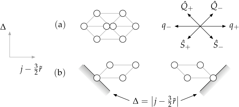
Figure 1: Multiplet structure of the super-Schrödinger algebra. (a) A long multiplet consists of eight conformal primary operators. (b) A short (chiral or anti-chiral) multiplet consists of four conformal primary operators.

An irreducible representation (irrep) of the super-Schrödinger algebra ${\bf sch_{2}^{(1)}}$ should consist of several irreps of the bosonic Schrödinger algebra ${\bf sch_{2}^{(0)}}$. As the dynamical part of the superalgebra contains three pairs of fermionic oscillators ($Q_{\pm},S_{\pm},q_{\pm}$), we expect generically eight irreps of the bosonic algebra to form a multiplet. As mentioned earlier, the irreps of the bosonic algebra are specified by their conformal primary states, so in order to specify a super-multiplet, it suffices to show how the eight primary states get mapped to each other by the super-charges.

The structure of a long multiplet of ${\bf sch_{2}^{(1)}}$ is depicted in Figure 1(a). We begin with the primary state $|1\rangle$ with the lowest value of $\Delta_{\cal O}$. By assumption it satisfies $\hat{L}_{-1}|1\rangle=\hat{G}_{\pm}|1\rangle=\hat{S}_{\pm}|1\rangle=0$. We further assume that $q_{-}|1\rangle=0$. When $N_{\cal O}\neq 0$, we can rescale the generators such that

$$\{q_{+},q_{-}\}=1,\qquad{}[\hat{G}_{\pm},\hat{P}_{\mp}]=2,$$ (4.29)

with other commutation relations unchanged. Then $|1\rangle$ is naturally paired with another primary operator $|2\rangle=q_{+}|1\rangle$ with the same $\Delta_{\cal O}$. Thus a generic (long) multiplet is specified by a pair of superconformal primary ($\hat{S}_{\pm}|\psi\rangle=0$) states. The remaining six primary states in the multiplet can be written explicitly as follows:

$$|3\rangle=-\hat{Q}_{+}|1\rangle\,, |4\rangle=\hat{Q}_{+}|2\rangle-\hat{P}_{+}|1\rangle\,,$$

$$|5\rangle=\hat{Q}_{-}|1\rangle-\hat{P}_{-}|2\rangle\,, |6\rangle=-\hat{Q}_{-}|2\rangle\,,$$

$$|7\rangle=\hat{Q}_{-}|3\rangle-\hat{Q}_{+}|5\rangle-\hat{P}_{-}|4\rangle\,, |8\rangle=\hat{Q}_{+}|6\rangle-\hat{Q}_{-}|4\rangle-\hat{P}_{+}|5\rangle\,.$$ (4.30)

It is easy to show that all of these are primary and have finite norm. They also satisfy $q_{+}|2k-1\rangle=|2k\rangle$. Note that, in general, the action of $\hat{Q}_{\pm}$ or $\hat{S}_{\pm}$ on a primary state in a multiplet yields a linear combination of other primary states as well as some descendants.

This structure should be augmented by the fact that our ${\cal N}=6$ algebra ${\bf sch_{2}^{(2)}}$ includes additional supercharges $q^{ai}_{\pm}$ and the $SU(2)\times SU(2)$ $R$-symmetry generators. However, since these generators commute with the dynamical generators, we can simply take the tensor product of the irreps on each side. We will come back to the representation theory of the ($q^{ai}_{\pm},R_{1},R_{2}$) subalgebra shortly.

Next, let us consider unitarity constraints of the super-Schrödinger algebra. Note that for any state $|\Psi_{\cal O}\rangle=e^{-H}{\cal O}|0\rangle$ of charges $\Delta_{\cal O},j_{\cal O},N_{\cal O},r_{\cal O}$,

$$||\hat{Q}_{\pm}|\Psi_{\cal O}\rangle||^{2}+||\hat{S}_{\mp}|\Psi_{\cal O}\rangle||^{2}=\langle\Psi_{\cal O}|\{\hat{S}_{\mp},\hat{Q}_{\pm}\}|\Psi_{\cal O}\rangle\geq 0,$$ (4.31)

which leads to an inequality

$$\Delta_{\cal O}\geq\left|j_{\cal O}-\frac{3}{2}r_{\cal O}\right|.$$ (4.32)

The bound is saturated by three types of short multiplets.

I. chiral operators or states for which

$$\Delta_{\cal O}=j_{\cal O}-\frac{3}{2}r_{\cal O}\Longrightarrow[Q_{-},{\cal O}]=[S_{+},{\cal O}]=0\ {\rm and}\ \hat{Q}_{-}|\Psi_{\cal O}\rangle=\hat{S}_{+}|\Psi_{\cal O}\rangle=0,$$ (4.33)

II. anti-chiral operators or states for which

$$\Delta_{\cal O}=-j_{\cal O}+\frac{3}{2}r_{\cal O}\Longrightarrow[Q_{+},{\cal O}]=[S_{-},{\cal O}]=0\ {\rm and}\ \hat{Q}_{+}|\Psi_{\cal O}\rangle=\hat{S}_{-}|\Psi_{\cal O}\rangle=0,$$ (4.34)

III. vacuum operators or states for which

$$\Delta_{\cal O}=\ j_{\cal O}-\frac{3}{2}r_{\cal O}=0\Longrightarrow[Q_{\pm},{\cal O}]=[S_{\pm},{\cal O}]=0\ {\rm and}\ \hat{Q}_{\pm}|\Psi_{\cal O}\rangle=\hat{S}_{\pm}|\Psi_{\cal O}\rangle=0.$$ (4.35)

The identity operator (vacuum state) with zero spin and zero $R$-charge appears to be the only vacuum operator in our theory.

One sees chiral primary operators (states) and anti-chiral primary operators saturate the unitarity bound. There are also the chiral descendant operators that are chiral (i.e. saturate the bound) but not superconformal primary. The chiral descendants can be obtained from the chiral primaries by multiple applications of $\hat{P}_{+}$, which increases not only $\Delta$ but also angular momentum $j$. The chiral primary and descendant states contribute to the superconformal index we will discuss in section 4.4.

One can build a short representation of the super-Schrödinger algebra ${\bf sch_{2}^{(1)}}$ starting from a given chiral primary state. Each short multiplet contains four primary states, as shown in 1. If the theory admits a continuous deformation, the dimension $\Delta_{\cal O}$ of a long multiplet may be lowered until it hits the unitarity bound. Then the long multiplet can split into two short multiplets. The pattern of the splitting should can be seen clearly in Figure 1, (a) and (b).

Finally, let us turn to the representation of the superalgebra ${\bf sch_{2}^{(2)}}$ whose kinematical supercharges satisfy the algebra

$$\{q_{-}^{\ ai},q_{+bj}\}=\frac{1}{2}\delta^{a}_{b}\delta^{i}_{j}{\cal N}-\delta^{a}_{b}R^{i}_{\ j}+\delta^{i}_{j}R^{a}_{\ b}.$$ (4.36)

where $R^{a}_{\ b},R^{i}_{\ j}$ denote generators of R-symmetry group $SU(2)\times SU(2)$. Its representation theory has been studied in [39]. For self-containedness, we review it in our context.

In a given irreducible representation of algebra ${\bf sch_{2}^{(1)}}$, let us choose any primary state $|\Psi\rangle$ of number charge $N$ and possible lowest angular momentum $j_{0}$ which transforms as an irreducible representation $(r_{1},r_{2})$ of two $SU(2)$’s. The operators $q^{ai}_{-}$ and $q_{+ai}$ lowers and raises the angular momentum $j$ by 1/2, respectively, but does not change the eigenvalues of $(J-\frac{3}{2}\tilde{R})$. As $|\Psi\rangle=|N,j_{0},r_{1},r_{2}\rangle$ has the lowest angular momentum,

$$q_{-}^{\ ai}|N,j_{0},r_{1},r_{2}\rangle=0,\ \text{for all}\ \ a,i\ .$$ (4.37)

For the unitarity, one has to demands that the matrix below

$$\langle\Psi^{\prime}|q_{-}^{\ ai}q_{+bj}|\Psi\rangle=\frac{1}{2}\delta^{a}_{b}\delta^{i}_{j}\langle\Psi^{\prime}|{\cal N}|\Psi\rangle-\delta^{a}_{b}\langle\Psi^{\prime}|R^{i}_{\ j}|\Psi\rangle+\delta^{i}_{j}\langle\Psi^{\prime}|R^{a}_{\ b}|\Psi\rangle.$$ (4.38)

has only non negative eigenvalues. After a suitable diagonalization, one can obtain the lower bound on number charge ${\cal N}$

$${\cal N}\geq 2~{}\text{max}\left[\Big{(}c_{2}\big{(}r_{1}\big{)}+c_{2}\big{(}\frac{1}{2}\big{)}-c_{2}\big{(}r^{\prime}_{1}\big{)}\Big{)}+\Big{(}c_{2}\big{(}r^{\prime}_{2}\big{)}-c_{2}\big{(}r_{2}\big{)}-c_{2}\big{(}\frac{1}{2}\big{)}\Big{)}\Big{|}\ r_{i}\otimes\frac{1}{2}=\oplus r^{\prime}_{i}\right]\ ,$$ (4.39)

where $c_{2}(r)$ is the quadratic Casimir of $SU(2)$ representation $r$, normalized such that $c_{2}(r)=r(r+1)$. The above bound is saturated when $c_{2}(r^{\prime}_{1})$ takes the smallest value while $c_{2}(r^{\prime}_{2})$ takes the largest one. The unitary restriction on number charge ${\cal N}$ is therefore given by

$$\left\{\begin{array}[]{lc}{\cal N}\geq 2\big{(}r_{1}+r_{2}+1\big{)}&(r_{1}\neq 0)\\ {\cal N}\geq 2r_{2}&(r_{1}=0)\end{array}\right.\ .$$ (4.42)

Applying the operators $q_{+ai}$ changes the representations $r_{1},r_{2}$ by $\pm 1/2$, and so generates $2^{4}(2r_{1}+1)(2r_{2}+1)$ primary states for the same $\Delta$ and $(J-\frac{3}{2}\tilde{R})$ eigenvalues:

• $j=j_{0}$ or $j_{0}+2$ : $(r_{1},r_{2})$ .

• $j=j_{0}+1/2$ or $j_{0}+3/2$ : $(r_{1}\pm 1/2,r_{2}\pm 1/2)$ .

• $j=j_{0}+1$ : $(r_{1},r_{2}\pm 1)\oplus(r_{1}\pm 1,r_{2})\oplus 2(r_{1},r_{2})$ .

Of course, if some of $r_{1}$ or $r_{2}$ is less than or equal to $1/2$, the number of the derived representations would be reduced as some of the derived irreducible representations does not exist. When the starting state is close to saturate the number unitary bound (4.42), then again some of the number of the derived states would become null and the number of derived states would be reduced.

We say the superconformal primary operators is bps operators or states if the above number unitary bound (4.42) is saturated. Those states are now annihilated by some of creation operators $q_{+ai}$ in such a manner as to give us the smallest $c_{2}(r_{1}^{\prime})$ and largest $c_{2}(r_{2}^{\prime})$. The resulting multiplet contains a total of $2^{3}(4r_{1}r_{2}+r_{1}+3r_{2}+1)$ states, which can be decomposed into the following bosonic irreps:

• $j=j_{0}$ : $(r_{1},r_{2})$.

• $j=j_{0}+1/2$ : $(r_{1}+1/2,r_{2}+1/2)\oplus(r_{1}-1/2,r_{2}-1/2)\oplus(r_{1}+1/2,r_{2}-1/2)$.

• $j=j_{0}+1$ : $(r_{1}+1,r_{2})\oplus(r_{1},r_{2}-1)\oplus(r_{1},r_{2})$.

• $j=j_{0}+3/2$: $(r_{1}+1/2,r_{2}-1/2)$.

Again the above derivation would be reduced if $r_{1}$ or $r_{2}$ is less than or equal to 1/2.

For a fixed value of $(r_{1},r_{2})$, a long multiplet can split into two short multiplets if the value of $N_{\cal O}$ is lowered to saturate the bps bound (4.42). If we denote the multiplets by $[N_{\cal O},r_{1},r_{2}]_{\rm long/short}$, the splitting rule is ($N_{\cal O}=2(r_{1}+r_{2}+1)$)

$$[N_{\cal O},r_{1},r_{2}]_{\rm long} \rightarrow [N_{\cal O},r_{1},r_{2}]_{\rm short}+[N_{\cal O},r_{1}-1/2,r_{2}+1/2]_{\rm short}\,,$$

$$2^{4}(2r_{1}+1)(2r_{2}+1) = 2^{3}(4r_{1}r_{2}+r_{1}+3r_{2}+1)+2^{3}(4r_{1}r_{2}+3r_{1}+r_{2}+1)\,.$$ (4.43)

4.3 Elementary fields and states

For the $U(1)\times U(1)$ theory, we can introduce the magnetic flux operator and multiply it to the fields $z_{\alpha},\psi^{\alpha}$ to make them gauge invariant. The flux operator carries fractional magnetic flux, making the physical operator to be quasi-local. However these charge-flux composite operators are not of anyonic ones with fractional spin and statistics, as the charge and the flux do not know each other.

Table 3: Charges for the physical fields in $U(1)\times U(1)$ theory

	$\Delta$	$J$	$2R$	$2\Sigma$	$\tilde{R}=(4R+2\Sigma)/3$	$J-\frac{3}{2}\tilde{R}$
$\bar{z}^{a}$	$1$	$0$	$+1$	$0$	$+2/3$	$-1$
$\bar{z}^{i}$	$1$	$0$	$-1$	$0$	$-2/3$	$+1$
$\bar{\psi}_{a}$	$1$	$+1/2$	$-1$	$+1$	$-1/3$	$+1$
$\bar{\psi}_{i}$	$1$	$-1/2$	$+1$	$-1$	$+1/3$	$-1$

Table 4: Physical fields under the supersymmetry

	$Q_{+}$	$Q_{-}$	$q_{+}$	$q_{-}$
$\bar{z}^{a}$	$0$	$-i\epsilon^{ab}D_{-}\bar{\psi}_{b}$	$-\epsilon^{ab}\bar{\psi}_{b}$	$0$
$\bar{z}^{i}$	$i\epsilon^{ij}D_{+}\bar{\psi}_{j}$	$0$	$0$	$\epsilon^{ij}\bar{\psi}_{j}$
$\bar{\psi}_{a}$	$-i\epsilon_{ab}D_{+}\bar{z}^{b}$	$0$	$0$	$-\epsilon_{ab}\bar{z}^{b}$
$\bar{\psi}_{i}$	$0$	$i\epsilon_{ij}D_{-}\bar{z}^{j}$	$\epsilon_{ij}\bar{z}^{j}$	$0$

For convenience, we summarize the relevant charges of physical fields in Table 3 and the kinematical/dynamical supercharges by which physical fields are annihilated in Table 4.

One can analyze what representation the creation operators in the $U(1)\times U(1)$ theory form under the super Schrödinger algebra ${\bf sch_{2}^{(2)}}$. One can see that elementary physical fields at the origin saturate the scaling-dimension bound (4.32) and are split to chiral and anti-chiral primary operators. Also they saturate the number bound (4.42) and so are bps operators:

$$\begin{array}[]{lll}\bar{z}^{i}(0),\bar{\psi}_{+a}(0):&(1/2,0)&\text{bps chiral primary}\\ \bar{z}^{a}(0),\bar{\psi}_{-i}(0):&(0,1/2)&\text{bps anti-chiral primary}\end{array}$$ (4.46)

In the ${\cal N}=4$ language, the first set of the fields $\bar{z}^{i},\bar{\psi}_{a}$ came from the twisted hyper-multiplet and the second set of the field $\bar{z}^{a},\bar{\psi}_{i}$ came from the hyper-multiplet. The products of chiral fields $\bar{z}^{i}$ and $\bar{\psi}_{a}$ will remain chiral primary. In addition, they would saturate the number bound (4.42) if one symmetrizes the $SU(2)\times SU(2)$ indices.

The hamiltonian $\hat{L}_{0}$ has a harmonic potential. Let us imagine a bunch of particles rotating around the origin in circular orbits. The radial kinetic energy can be ignored and the total energy would be roughly

$$\Delta\sim\frac{mw^{2}}{2}r^{2}+\frac{J^{2}}{2mr^{2}}\,,$$ (4.47)

which is minimized when $J\sim mwr^{2}$. The energy becomes

$$\Delta\sim wJ\,.$$ (4.48)

Thus, our chiral states in large $\Delta$ limit may be represented by such configurations. Indeed, for $U(1)\times U(1)$ case, the chiral operator $\partial_{+}^{n}\bar{z}^{i}$ with large $n$ may represent such circular motion.

For a larger gauge group, we argued in Sec. 2 for the existence of the nonabelian flux-charge comoposte creation operators,

$$\bar{\cal Z}^{i},\ \bar{\varPsi}_{+a},\ \ \bar{\cal Z}^{a},\ \bar{\varPsi}_{-i}.$$ (4.49)

They are invariant under the local gauge transformation but transform as $N\times\bar{N}$ under the global part of the $U(N)\times U(N)$ gauge symmetry. They would discribe the creation operators for single massive particle. Thus their spin and R-quantum number would be more and less identical to that of the abelian case. Thus these operators would be also bps (anti-)chiral operators. In addition, as they carry the fractional nonabelian magnetic flux, these composite operators may be quasi-local in the sense their statitics may be fractional. It would be interesting to construch such operators explicitly, at least perturbatively in the weak coupling or large $k$ regime, and to explore their two point functions.

In addition, the quantum partners of the classical BPS configuration of our Lagrangian would play a special role. The detail study of the classical BPS configurations need? some attention. In our theory there exist di-baryonic operators, say, made of only the scalar fields $z^{\ A}_{a\ M}(0)$ without any flux attached, which would be invariant under the local gauge transformation, and also singlet under the global part of the gauge group. These di-baryonic operators would remain chiral.

4.4 Comments on the superconformal index

Using the operator-state correspondence, one can naturally define a nonrelativistic superconformal Witten index [29] in analogy with the relativistic counterpart [40], which counts the chiral states that are annihilated by $\hat{Q}_{-},\hat{S}_{+}$. They are made of chiral primary and descendant states. For general states, there are two bounds (4.32) and (4.42). The first bound is saturated by the chiral states. In addition, there are many ways to discern these chiral states by measuring their additional charges. The examples are

$$\Delta+2J,\ N-2(r_{1}+r_{2}),r_{1}-r_{2},\ m_{1},\ m_{2},$$ (4.50)

which commute with $Q_{-},S_{+}$. The index we want to compute is therefore given by

$${\cal I}(x,y_{1},y_{2})=\lim_{\beta\rightarrow\infty}{\rm Tr}\Big{[}(-1)^{F}e^{-\beta(\Delta-(j-\frac{3}{2}r))}e^{\mu(N-2(r_{1}+r_{2}))}x^{\Delta+2j}y_{1}^{m_{1}}y_{2}^{m_{2}}y_{3}^{r_{1}-r_{2}}\Big{]}$$ (4.51)

In the $\mu\rightarrow-\infty$ limit, the above index counts only $bps$ states.

The superconformal index of a relativistic theory in the limit of vanishing coupling can be computed in two steps [40]. One begins by computing the index for chiral ‘letters’, namely, elementary fields and derivatives without worrying about gauge invariance. The result is then inserted into a matrix integral which efficiently picks out the gauge invariant combinations among products of elementary fields and derivatives.

The chiral ($\Delta-J+\frac{3}{2}\tilde{R}\doteq 0$) ‘letters’ of the nonrelativistic ABJM model are just $\bar{z}^{i},\bar{\psi}_{a}$ and covariant derivatives $D_{+}$. Note that the field strength is not chiral. The fields $z_{a},\psi^{i}$ also have the correct quantum numbers to become chiral letters, but since they are annihilation operators, they could not contribute to creating an energy eigenstate of the many body system in a harmonic potential. If we stick to $\bar{z}^{i}$ and $\bar{\psi}_{a}$ only, we could not form any gauge-invariant ‘mesonic’ operators (trace of products of bi-fundamental fields). The ‘di-baryonic’ operators involving determinants of the $U(N)\times U(N)$ gauge groups are not affected. It is possible to count the mesonic operators in the $N=0$ section as done in Ref. [29], but its physical interpretation seems unclear to us.

We think that the flux-charge composite operators $\bar{{\cal Z}}^{i},\bar{\varPsi}_{a}$ remain chiral even in the nonabelian case as in the abelian case. They are invariant under the local gauge transformation, but become bi-fundamental under the global part of the gauge group. These operators would create the chiral states and would contribute to the chiral index. It would be very interesting to find out whether this is the case in the large $k$ limit where the Gauss law becomes simpler.

Acknowledgment

It is our pleasure to thank Eoin Ó Colgáin, Hossein Yavartanoo, Rajesh Gopakumar and Seok Kim for helpful discussions. We also thank to Yu Nakayama for discussions on subtleties in superconformal index. KML is supported in part by the KOSEF SRC Program through CQUeST Sogang University and KRF-2007-C008 program. Sm.L. is supported in part by the KOSEF Grant R01-2006-000-10965-0 and the Korea Research Foundation Grant KRF-2007-331-C00073.

References

• [1] D.T. Son, “Toward an AdS/cold atoms correspondence: a geometric realization of the Schroedinger symmetry,” Phys. Rev.  D 78, 046003 (2008) [arXiv:0804.3972 [hep-th]].
• [2] K. Balasubramanian and J. McGreevy, “Gravity duals for non-relativistic CFTs,” Phys. Rev. Lett.  101, 061601 (2008) [arXiv:0804.4053 [hep-th]].
• [3] C.P. Herzog, M. Rangamani and S.F. Ross, “Heating up Galilean holography,” JHEP 0811, 080 (2008) [arXiv:0807.1099 [hep-th]].
• [4] J. Maldacena, D. Martelli and Y. Tachikawa, “Comments on string theory backgrounds with non-relativistic conformal symmetry,” JHEP 0810, 072 (2008) [arXiv:0807.1100 [hep-th]].
• [5] A. Adams, K. Balasubramanian and J. McGreevy, “Hot Spacetimes for Cold Atoms,” JHEP 0811, 059 (2008) [arXiv:0807.1111 [hep-th]].
• [6] S. A. Hartnoll and K. Yoshida, “Families of IIB duals for nonrelativistic CFTs,” JHEP 0812, 071 (2008) [arXiv:0810.0298 [hep-th]].
• [7] A. Donos and J.P. Gauntlett, “Supersymmetric solutions for non-relativistic holography,” arXiv:0901.0818 [hep-th].
• [8] C.R. Hagen, “Scale and conformal transformations in galilean-covariant field theory,” Phys. Rev.  D 5, 377 (1972).
• [9] U. Niederer, “The maximal kinematical invariance group of the free Schrodinger equation,” Helv. Phys. Acta 45, 802 (1972).
• [10] Y. Nishida and D.T. Son, “Nonrelativistic conformal field theories,” Phys. Rev.  D 76, 086004 (2007) [arXiv:0706.3746 [hep-th]].
• [11] O. Aharony, O. Bergman, D. L. Jafferis and J. Maldacena, “${\cal N}=6$ superconformal Chern-Simons-matter theories, M2-branes and their gravity duals,” arXiv:0806.1218 [hep-th].
• [12] K. Hosomichi, K.M. Lee, S. Lee, S. Lee and J. Park, “${\cal N}=4$ superconformal Chern-Simons theories with hyper and twisted hyper multiplets,” JHEP 0807, 091 (2008) arXiv:0805.3662 [hep-th].
• [13] K. Hosomichi, K.M. Lee, S. Lee, S. Lee and J. Park, “${\cal N}=5,6$ superconformal Chern-Simons theories and M2-branes on orbifolds,” arXiv:0806.4977 [hep-th].
• [14] J. Gomis, D. Rodriguez-Gomez, M. Van Raamsdonk and H. Verlinde, “A massive study of M2-brane proposals,” arXiv:0807.1074 [hep-th].
• [15] J. Bagger and N. Lambert, “Modeling multiple M2’s,” Phys. Rev.  D 75, 045020 (2007) [arXiv:hep-th/0611108].
• [16] J. Bagger and N. Lambert, “Gauge symmetry and supersymmetry of multiple M2-branes,” Phys. Rev.  D 77, 065008 (2008) arXiv:0711.0955 [hep-th].
• [17] J. Bagger and N. Lambert, “Comments On multiple M2-branes,” JHEP 0802, 105 (2008) arXiv:0712.3738 [hep-th].
• [18] A. Gustavsson, “Algebraic structures on parallel M2-branes,” arXiv:0709.1260 [hep-th].
• [19] A. Gustavsson, “Selfdual strings and loop space Nahm equations,” JHEP 0804, 083 (2008) arXiv:0802.3456 [hep-th].
• [20] J. Gomis, A. J. Salim and F. Passerini, “Matrix theory of type IIB plane wave from membranes,” JHEP 0808, 002 (2008) [arXiv:0804.2186 [hep-th]].
• [21] K. Hosomichi, K. M. Lee and S. Lee, “Mass-deformed Bagger-Lambert theory and its BPS objects,” arXiv:0804.2519 [hep-th].
• [22] I. Bena, “The M-theory dual of a 3 dimensional theory with reduced supersymmetry,” Phys. Rev.  D 62, 126006 (2000) [arXiv:hep-th/0004142].
• [23] I. Bena and N. P. Warner, “A harmonic family of dielectric flow solutions with maximal supersymmetry,” JHEP 0412, 021 (2004) [arXiv:hep-th/0406145].
• [24] R. Jackiw and S.Y. Pi, “Classical and quantal nonrelativistic Chern-Simons theory,” Phys. Rev.  D 42, 3500 (1990) [Erratum-ibid.  D 48, 3929 (1993)].
• [25] M. Leblanc, G. Lozano and H. Min, “Extended superconformal Galilean symmetry in Chern-Simons matter systems,” Annals Phys.  219, 328 (1992) [arXiv:hep-th/9206039].
• [26] M. Sakaguchi and K. Yoshida, “Super Schrodinger in Super Conformal,”arXiv:0805. 2661 [hep-th].
• [27] M. Sakaguchi and K. Yoshida, “More super Schrodinger algebras from $psu(2,2|4)$,” JHEP 0808, 049 (2008) [arXiv:0806.3612 [hep-th]].
• [28] M. Sakaguchi and K. Yoshida, “Super Schroedinger algebra in AdS/CFT,” J. Math. Phys.  49 (2008) 102302.
• [29] Y. Nakayama, “Index for non-relativistic superconformal field theories,” JHEP 0810, 083 (2008) [arXiv:0807.3344 [hep-th]].
• [30] Y. Nakayama, S. Ryu, M. Sakaguchi and K. Yoshida, “A family of super Schrodinger invariant Chern-Simons matter systems,” JHEP 0901, 006 (2009) [arXiv:0811.2461 [hep-th]].
• [31] G. V. Dunne, R. Jackiw, S. Y. Pi and C. A. Trugenberger, “Selfdual Chern-Simons solitons and two-dimensional nonlinear equations,” Phys. Rev.  D 43 (1991) 1332 [Erratum-ibid.  D 45 (1992) 3012].
• [32] G. V. Dunne, R. Jackiw and C. A. Trugenberger, “Chern-Simons theory in the Schrödinger representation,” Annals Phys.  194 (1989) 197.
• [33] S. Elitzur, G. W. Moore, A. Schwimmer and N. Seiberg, “Remarks on the canonical quantization of the Chern-Simons-Witten theory,” Nucl. Phys.  B 326 (1989) 108.
• [34] H. Lin and J.M. Maldacena, “Fivebranes from gauge theory,” Phys. Rev.  D 74, 084014 (2006) [arXiv:hep-th/0509235].
• [35] A. Agarwal, N. Beisert and T. McLoughlin, “Scattering in mass-deformed ${\cal N}\geq 4$ Chern-Simons Models,” arXiv:0812.3367 [hep-th].
• [36] M. Henkel, “Schrodinger invariance in strongly anisotropic critical systems,” J. Statist. Phys.  75, 1023 (1994) [arXiv:hep-th/9310081].
• [37] A. Bagchi and R. Gopakumar, “Galilean conformal algebras and AdS/CFT,” arXiv:0902.1385 [hep-th].
• [38] V. de Alfaro, S. Fubini and G. Furlan, “Conformal Invariance In Quantum Mechanics,” Nuovo Cim.  A 34 (1976) 569.
• [39] N. Beisert, “The analytic Bethe ansatz for a chain with centrally extended $su(2|2)$ Symmetry”, J. Stat. Mech. 07, P01017 (2007), [arXiv:nlin.SI/0610017].
• [40] J. Kinney, J.M. Maldacena, S. Minwalla and S. Raju, “An index for 4 dimensional super conformal theories,” Commun. Math. Phys.  275, 209 (2007) [arXiv:hep-th/0510251].
• [41] J. Bhattacharya and S. Minwalla, “Superconformal indices for ${\cal N}=6$ Chern Simons theories,” JHEP 0901, 014 (2009) [arXiv:0806.3251 [hep-th]].
• [42] F. A. Dolan, “On Superconformal Characters and Partition Functions in Three Dimensions,” arXiv:0811.2740 [hep-th].
• [43] J. Choi, S. Lee and J. Song, “Superconformal indices for orbifold Chern-Simons theories,” arXiv:0811.2855 [hep-th].
• [44] Y. Nakayama, M. Sakaguchi and K. Yoshida, “Non-Relativistic M2-brane Gauge Theory and New Superconformal Algebra,” arXiv:0902.2204 [hep-th].