Analysis of the conduction heat transfer in cantilevers under steady state cryogenic conditions

Abstract

An accurate analysis of the conduction heat transfer in a cryogenic flask is made and some useful formulae are derived. Taking into account the temperature dependence of conductivity and tensile strength of the supporting rods for a helium cryostat, these formulae may provide more exact results than the the formulae based on simpler models. This allows the design of the supporting elements of a liquid helium cryostat with minimum cross-section (for minimizing the heat transfer)and proper mechanical resistance. Some examples of numerical results and tables are also presented.

I Introduction

Although the heat transfer theory is well known for ordinary conditions Fou and a huge number of studies and applications may be found, there is still a lack of experimental data and theoretical solutions for the problem of the heat transfer in cryogenic systems. Taking into account the continuous development of the cryogenic techniques Leb and their applications especially in superconductor systems, it becomes more and more important to minimize the heat transfer flux and hence the loss of cryogenic liquids in such installations.

There are two processes that enable the heat transfer to a liquid helium cryostat built as a Dewar flask :conduction and radiation.In figure 1 we present a possible structure of the cryostat, and one may see that the conduction process appears due to the sustaining elements of the inner flask. In order to minimize the heat transfer towards such an element it has to be made using a thermal insulating material with a cross section as small as possible. Unfortunately this reduces the mechanical resistance of the supports, especially at cryogenic temperatures 1 . Various materials have been experimented and it seems that the austenitic steels are quite adequate for this purpose, despite their relatively high thermal conductivity. Since the tests for an optimal structure are expensive due to the liquid helium evaporation that inevitably occurs, it would be desirable to numerically estimate the heat transfer for various materials, shapes and dimensions, in order to avoid as much as possible the experimental optimization of the system.

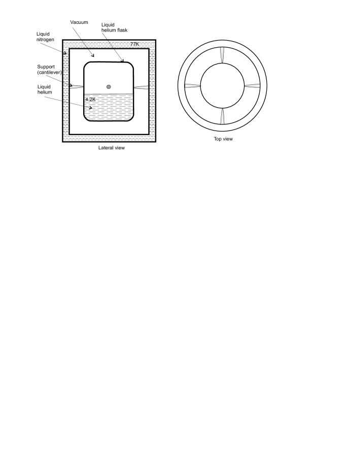
Figure 1: A typical Dewar flask for liquid helium

However, the usual formulae for heat transfer in rods and for their mechanical characteristics fail in cryogenic regime, due to the variation with the temperature of the conductance 2 and tensile strength of the materials 3 . The aim of this paper is to include as accurate as possible these variations in the formulae necessary for the optimal design.

II Heat transfer in a variable profile cantilever under cryogenic conditions

We are interested in calculating the rate of heat transfer in a rod placed in vacuum and with the extremities kept at two different constant temperatures, $T_{1}=4.2$K and $T_{2}=77$K in steady state conditions.

The heat transfer rate may be described by the Fourier law which states that this is proportional to the gradient in temperature and to the normal area through which the heat is flowing

$$\vec{J}=-KS\nabla T$$ (1)

where:

$\bullet\vec{J}$ is the rate of heat transfer (heat flux)[Wm^-2]

$\bullet K$ is the conductivity of the material (constant)[Wm^-3K^-1]

$\bullet S$ is the cross section of the rod (constant)[m²]

$\bullet\nabla T$ is the gradient in temperature [Km^-1].

As there is no conduction heat transfer at the lateral surface of the rod placed in vacuum, the problem is one-dimensional and the solution may be written as

$$J=\frac{{dQ}}{{dt}}=K\cdot S\frac{{(T_{2}-T_{1})}}{L}$$ (2)

where

$\bullet T_{1}$ and $T_{2}$ are the constant temperatures at the rod’s edges [K]

$\bullet L$ is the length of the rod [m]

This equation is valid only for constant cross section and conductivity of the rod and small temperature difference. If this is not the case, one must divide the whole rod in thin slices to ensure the validity of the eq. (2). Thus, we may write:

$$J=K\cdot S(x)\cdot\frac{{dT(x)}}{{dx}}$$ (3)

Taking also into account the dependence of the material’s conductivity with the temperature:

$$K=K(T(x))$$ (4)

the equation (3 ) becomes

$$J=K(T(x))S(x)\frac{{dT(x)}}{{dx}}$$ (5)

For cryogenic temperatures (lower than the Debye temperature), the mean free pass of the phonons may exceed the dimensions of the rod and hence the conductivity will be a function only of the specific heat capacity $C_{V}$ 2

$$K(T)=\chi C_{V}(T)$$ (6)

where the constant $\chi$ is a characteristic of the material.

According to the classical Debye model Deb , in this regime the specific heat capacity increases with the temperature as 2

$$C_{V}=aT^{3}$$ (7)

involving another material’s constant $a$.

More general, the Rosseland approximation Ros Ros1 allows considering also an additive constant $b$ due to the molecular conductivity

$$C_{v}=b+aT^{3}$$ (8)

As for $b=0$ the Debye dependence is found, we shall consider this more general formula with the parameter $b$ more or less significant for various materials.

From eqs. (5), (6) and (8) we obtain:

$$J=\chi[b+aT^{3}(x)]S(x)\frac{{dT(x)}}{{dx}}$$ (9)

Separating the variables we may now integrate this ordinary differential equation

$$J\frac{{dx}}{{S(x)}}=\chi[b+aT^{3}(x)]dT(x)$$ (10)

$$J\int\limits_{0}^{L}{\frac{{d(x)}}{{S(x)}}=\chi[b(T_{2}-T_{1})+\frac{a}{4}}(T_{2}^{4}-T_{1}^{4})]$$ (11)

where we took into account that the thermal flux $J$ is constant in steady-state conditions.

From equation (11) we obtain the heat transfer rate $J$ as:

$$J=\chi[b(T_{2}-T_{1})+\frac{a}{4}(T_{2}^{4}-T_{1}^{4})]\left[{\int\limits_{0}^{L}{\frac{{dx}}{{S(x)}}}}\right]^{-1}$$ (12)

We may also obtain the temperature distribution along the rod, which will be necessary for mechanical resistance calculations. From eq. (5) we may write

$$dT(x)=J\frac{{dx}}{{K(T(x))\cdot S(x)}}$$ (13)

At a distance $l$ from the $T_{1}$ source, the temperature $T(l)$ is obtained by integrating eq. (13)

$$\int\limits_{T_{1}}^{T(l)}{\chi[b+aT^{3}(x)]dT(x)=J\int\limits_{0}^{l}{\frac{{dx}}{{S(x)}}}}$$ (14)

$$\chi\{b[T(l)-T_{1}]+\frac{a}{4}[T^{4}(l)-T_{1}^{4}]\}=J\int\limits_{0}^{l}{\frac{{dx}}{{S(x)}}}$$ (15)

Using eq. (12) for the heat transfer rate $J$, the temperature distribution is given by the following equation, that may be solved numerically for obtaining the temperature distribution in the rod

$$bT(l)+\frac{a}{4}T^{4}(l)=bT_{1}+\frac{a}{4}T_{1}^{4}+[b(T_{2}-T_{1})+\frac{a}{4}(T_{2}^{4}-T_{1}^{4})]\left[{\int\limits_{0}^{L}{\frac{{dx}}{{S(x)}}}}\right]^{-1}\int\limits_{0}^{l}{\frac{{dx}}{{S(x)}}}$$ (16)

III Considerations concerning the profile of the cantilevers in cryogenic conditions

It is known that the general Euler-Bernoulli beam theory neglects the share deformations and the beam deflection is given by the equation

$$\frac{{\partial^{2}}}{{\partial x^{2}}}(EI\frac{{\partial^{2}u}}{{\partial x^{2}}})=F$$ (17)

where:

$\bullet E$ is the you Young modulus

$\bullet I$ is the second moment area

$\bullet F$is the distributed force (force per length)

The more general Timoshenko beam theory includes the shear forces leading to a coupled linear partial equations:

$$\rho A\frac{{\partial^{2}u}}{{\partial t^{2}}}=\frac{\partial}{{\partial x}}(AkG(\frac{{\partial u}}{{\partial x}}-\theta))+F$$ (18)

$$\rho I\frac{{\partial^{2}\theta}}{{\partial t^{2}}}=\frac{\partial}{{\partial x}}(EI\frac{{\partial\theta}}{{\partial x}})+AkG(\frac{{\partial u}}{{\partial x}}-\theta)$$ (19)

where:

$\bullet\rho$ is the density of beam material;

$\bullet A$is the cross-section area;

$\bullet G$ is the shear modulus;

$\bullet k$ is the Timoshenko shear coefficient;

The tensile stress in the beam at the distance $y$ from the neutral axis and in the same plane with the beam and the applied force is

$$\sigma=Ey\frac{{\partial^{2}u}}{{\partial x^{2}}}=\frac{{My}}{I}$$ (20)

where $M$ is the bending moment proportional with the distance to the applied force $F$(figure 2)

$$M=F(L-x)$$ (21)

Obviously the tensile stress must not exceed the tensile strength $\sigma_{max}$ which is a characteristic of the material, and in cryogenic regime depends on the temperature

Thus, from eqs. (20) and (21) it follows

$$\frac{{y_{\max}}}{I}F(L-x)\leq\sigma_{\max}$$ (22)

One may see that the tensile stress increases linearly with the distance to the applied force, being maximum at the fixed end of the cantilever and zero at the mobile end. So, a higher mechanical resistance is necessary towards the fixed end, meaning that the cantilever has to be ticker as $x$ decreases. We recall that the heat loss is increasing with the cross section of the cantilever, so that it must be kept as low as possible.

Obviously, the solution is to use a variable cross section area cantilever, thinner in the low tensile effort regions and thicker in the high tensile effort ones. The ideal dependence of this cross section should keep the same ratio between the allowed tensile stress and the actual one in every point among the beam. This will influence also the thermal conductivity of the cantilever and the heat transfer flux 4 .

For a variable cross section area of the beam, the second area moment area $I$ and $y_{max}$ are also variable.

For finding the optimal profile, we must first choose the shape of the cross-section and find the dependence of the second moment area on its geometrical characteristics.

In most cases, the applied force is in a fixed plane and an I shape cantilever provides the largest second moment area with a minimum cross section area. However, in our case if the flask is inclined, the applied force changes the relative plane and the I shape cantilever has a much lower admissible tensile stress in such situation.

That is why a circular or a rectangular shape of the cross section may be a proper choice, despite its lower performance in the one plane case.

a) Circular shape cross section cantilever

The second momentum area in this case is

$$I=\frac{{\pi r^{4}}}{4}$$ (23)

From eq. (1.21) with $y_{\max}=r$ we obtain

$$\frac{{4F}}{{\pi r^{3}}}(L-x)\leq\sigma_{\max}(T(x)$$ (24)

and the profile of the cantilever is given by

$$r(x)\geq[\frac{{4F}}{{\pi\sigma_{\max}(T(x))}}(L-x)]^{\frac{1}{3}}$$ (25)

Of course, one should choose a provision for the parameter $r$ (the radius must have a nonzero value $r_{0}$ at the mobile end) so that the recommended equation is

$$r(x)=r_{0}+[\frac{{4F}}{{\pi\sigma_{\max}(T(x))}}(L-x)]^{\frac{1}{3}}$$ (26)

In figure 2 is represented the recommended dependence of the radius on the distance to the fixed end. The most difficult part in this equation is generated by the dependence with the temperature of the maximum tensile strength of the material. Qualitatively, it is known that it decreases with the temperature decrease in cryogenic regime, but an exact formula for this dependence is not available. The problem may be solved only numerically or using some approximation. For numerically solving the whole problem, one must use a table containing the values of the tensile strength of the material for several temperature within the desired range. Now an approximating polynomial function may be obtained with high accuracy, using for example the method of Lagrange interpolation

$$\sigma_{\max}(T(x))=\sum\limits_{i=1}^{n}{\sigma_{\max}(}T_{i})\prod\limits_{\scriptstyle j=1\hfill\atop\scriptstyle j\neq i\hfill}^{n}{\frac{{T(x)-T_{j}}}{{T_{i}-T_{j}}}}$$ (27)

We plug in this function in eq. (26) and together with eq (12) we obtain a coupled nonlinear equations that should be solved numerically.

A simpler but less accurate solution is to approximate the dependence of the tensile stress with a first degree polynomial in variable $x$

$$\sigma_{\max}(T(x))=\sigma_{0}-cx$$ (28)

where the constant $c$ may be obtained as the slope of a line which best approximates the data in the mentioned table.

Thus, eq. (26) becomes

$$r=r_{0}+[\frac{{4F}}{{\pi(\sigma_{0}-cx)}}(L-x)]^{\frac{1}{3}}$$ (29)

Inserting this equation in (12) we obtain the following expression for the heat transfer rate in a cantilever with circular cross section and optimal profile

$$J=\chi[b(T_{2}-T_{1})+\frac{a}{4}(T_{2}^{4}-T_{1}^{4})]I_{1}$$ (30)

where $I_{1}=\left[{\int\limits_{0}^{L}{\frac{{dx}}{{S_{1}(x)}}}}\right]^{-1}$ has an exact analytical solution that may be expressed in terms of Gauss hypergeometric functions ${}_{2}F_{1}(a,b;c;z)$ 6

$$I_{1}=\frac{\sigma_{0}\sqrt[3]{\frac{4FL}{\sigma_{0}}+\pi r_{0}}\left[4\sqrt[3]{2}\,_{2}F_{1}\left(\frac{1}{3},\frac{1}{3};\frac{4}{3};\frac{4cFL+c\pi\sigma_{0}r_{0}}{4cFL-4F\sigma_{0}}\right)+\left(\frac{\sigma_{0}\left(4F+c\pi r_{0}\right)}{F(\sigma_{0}-cL)}\right)^{2/3}\right]}{\pi\left(4F+c\pi r_{0}\right)\left(-\frac{4F\sigma_{0}+c\pi r_{0}\sigma_{0}}{cFL\pi-F\pi\sigma_{0}}\right)^{2/3}}$$

$$+\frac{(cL-\sigma_{0})\sqrt[3]{r_{0}}\left[4\sqrt[3]{2}\,_{2}F_{1}\left(\frac{1}{3},\frac{1}{3};\frac{4}{3};-\frac{c\pi r_{0}}{4F}\right)+\left(\frac{c\pi r_{0}}{F}+4\right)^{2/3}\right]}{\left(4F+b\pi r_{0}\right)\left(\frac{c\pi r_{0}}{F}+4\right)^{2/3}}$$ (31)

b) Rectangular shape cross section cantilever

In the case of rectangular cross section, the second moment of area is

$$I(x)=\frac{{wh(x)^{3}}}{{12}}$$ (32)

where $w$ is the width (horizontal dimension) and $h$ is the height (vertical dimension) of the cantilever. Since the $h$ dimension has a greater influence to the overall resistance, only it will depend on $x$.

Plugging in this formula in eq. (22) and considering $y_{\max}(x)=\frac{{h(x)}}{2}$, we obtain

$$h(x)=[\frac{{6F}}{{w\sigma_{\max}}}(L-x)]^{\frac{1}{2}}+h_{0}$$ (33)

Again, taking into account the dependence on the temperature of the strength of the material, we may use the Lagrange interpolation formula (27) for a polynomial approximation, or be satisfied with the linear formula .In the last case, the profile equation becomes

$$h(x)=h_{0}+[\frac{{6F}}{{w(\sigma_{0}-bx)}}(L-x)]^{\frac{1}{2}}$$ (34)

Also, inserting this equation in (12) we obtain the following expression for the heat transfer rate in a cantilever with rectangular cross section and optimal profile

$$J=\chi[b(T_{2}-T_{1})+\frac{a}{4}(T_{2}^{4}-T_{1}^{4})]I_{2}$$ (35)

where $I_{2}=\left[{\int\limits_{0}^{L}{\frac{{dx}}{{wh(x)}}}}\right]^{-1}$ may be numerically calculated.

IV Numerical results and conclusions

Using our analytical formulae for the cross sections of the cantilever for an optimal mechanical resistance and minimal conduction we get the numerical numerical results in Table 1. We provided nonzero value at the mobile end, where the moment is theoretically null, to prevent the shearing deformation that was not included in the Bernoulli-Euler equation. No variation of the tensile strength with the temperature has been considered, so that higher values for the radius should be taken towards the mobile end. It suggests that a conical profile would be a good approximation for the optimum compromise between mechanical and thermal characteristics of the cantilever.

Table 1: The longitudinal variation of the radius (in mm) of an austenitic steel cantilever necessary for various weights of the liquid helium flask

x[m]	F=10N	F=20 N	F=30 N	F=40 N
0.01	3.68484	4.38268	4.8722	5.26191
0.02	3.63688	4.32226	4.80304	5.18579
0.03	3.58712	4.25957	4.73127	5.10679
0.04	3.53536	4.19436	4.65663	5.02464
0.05	3.4814	4.12637	4.5788	4.93898
0.06	3.42499	4.05529	4.49744	4.84943
0.07	3.36582	3.98074	4.4121	4.7555
0.08	3.30353	3.90227	4.32226	4.65663
0.09	3.23768	3.8193	4.22729	4.55209
0.10	3.1677	3.73114	4.12637	4.44102
0.11	3.0929	3.63688	4.01848	4.32226
0.12	3.01232	3.53536	3.90227	4.19436
0.13	2.92471	3.42499	3.77592	4.05529
0.14	2.82831	3.30353	3.63688	3.90227
0.15	2.72051	3.1677	3.4814	3.73114
0.16	2.59718	3.01232	3.30353	3.53536
0.17	2.45113	2.82831	3.0929	3.30353
0.18	2.26768	2.59718	2.82831	3.01232
0.19	2.00616	2.26768	2.45113	2.59718
0.20	2.00000	2.00000	2.00000	2.00000

The proposed formulae may be used for a proper design of the liquid helium recipient in order to minimize the heat transfer and preserve the mechanical characteristics of the system. They include the conduction and tensile strength dependance on the temperature in cryogenic regime which may be theoretically estimated or experimentally determined for the material of choice. Although they lead to a cumbersome profile of the cantilever, a good approximation with a conical one may be considered for practical purpose, assuming that the actual cross section is grater or equal to that predicted by our formulae in every point.

Figure 2: The optimal cantilever profile for a circular cross section

- (1) J. Fourier, J. The Analytical Theory of Heat. Dover Publications Inc. New York, 1955;
- (2) P. Lebrun, Advanced superconducting technology for global science: the Large Hadron Collider at CERN, Adv. Cryog. Eng., 47A: 3-14 (2002);
- (3) G. Claudet , Superfluid helium from physics laboratory to industry, Proceedings of ICEC19, Gistau-Seyfert ed., Narosa Publishing House, New Delhi: 743-750 (2002);
- (4) D. G. Cahill and R. O. Pohl, ”Lattice Vibrations and Heat Transport in Crystals and Glasses,” Ann. Rev. Phys. Chem. 39: 93-121, (1988);
- (5) P. Debye,Zur Theorie der spezifischen Waerme, Annalen der Physik (Leipzig) 39(4), p. 789 (1912);
- (6) S. Rosseland, Ap Phys J, 61, 424,(1925);
- (7) S. Rosseland, ”The Principles of Quantum Theory”, Erg nzungsband, pp. 243-249, (1936);
- (8) M. R. Sridhar and M. M. Yovanovich, ”Thermal Contact Conductance of Tool Steel and Comparison with Model,” Int. J. of Heat Mass Transfer 39 (4): 831-839, (1996);
- (9) M. M. Yovanovich, P. Teertstra, and J. R. Culham, ”Modeling Transient Conduction From Isothermal Convex Bodies of Arbitrary Shape,” Journal of Thermophysics and Heat Transfer 9 (3): 385-390, 1995;
- (10) M. Abramowitz and I. A. Stegun, Handbook of Mathematical Functions, Dover, New York, 1965.