Abstract

In this letter we discuss the analyticity properties of the Wilson–loop correlation functions relevant to the problem of soft high–energy scattering, directly at the level of the functional integral, in a genuinely nonperturbative way. The strategy is to start from the Euclidean theory and to push the dependence on the relevant variables $\theta$ (the relative angle between the loops) and $T$ (the half–length of the loops) into the action by means of a field and coordinate transformation, and then to allow them to take complex values. In particular, we determine the analyticity domain of the relevant Euclidean correlation function, and we show that the corresponding Minkowskian quantity is recovered with the usual double analytic continuation in $\theta$ and $T$ inside this domain. The formal manipulations of the functional integral are justified making use of a lattice regularisation. The new rescaled action so derived could also be used directly to get new insights (from first principles) in the problem of soft high–energy scattering.

1 Introduction

In recent years, starting from the seminal paper [1] by O. Nachtmann, the long–standing problem of soft high–energy scattering in strong interactions has been approached in the framework of nonperturbative QCD, with functional–integral techniques (for a review see Refs. [2, 3]). In this approach the parton–parton elastic scattering amplitudes, at high center–of–mass energy $\sqrt{s}\gg 1{\rm GeV}$ and small transferred momentum $\displaystyle\sqrt{|t|}\lesssim 1{\rm GeV}$, are described by certain (properly normalised) correlation functions of two infinite lightlike Wilson lines, running along the classical trajectories of the colliding partons [1, 4, 5, 6, 7]. These correlation functions suffer from infrared (IR) divergences [4, 5], which can be regularised considering Wilson lines of finite length $2T$ along the classical trajectories of partons with non–zero mass $m$, so forming a finite hyperbolic angle $\chi{\simeq}\log(s/m^{2})$ (for ${s\to\infty}$) in Minkowski space–time [4, 5, 8, 9, 10]. IR divergences can be avoided from the onset, considering instead the elastic scattering amplitude of two colourless states, e.g. two $q\bar{q}$ meson states, which is expected to be an IR–finite quantity [11]. It has been shown in [12, 13, 14, 15] (see also [2, 3]) that in this case the meson–meson elastic scattering amplitudes can be reconstructed from the correlation functions of two Wilson loops (which describe the scattering of two colour dipoles of fixed transverse size) running along the trajectories of the colliding hadrons, after folding them with appropriate wave functions describing the interacting mesons. In this letter we will be concerned with meson–meson elastic scattering only, and thus only with Wilson–loop correlation functions.

It has been shown in [8, 9, 10, 16, 17, 18] that, under certain analyticity hypotheses, the relevant correlation functions can be reconstructed from the “corresponding” correlation functions of two Euclidean Wilson lines or Wilson loops, of finite length $2T$, and forming an angle $\theta$ in Euclidean space, by means of the double analytic continuation $\theta\to-i\chi$, $T\to iT$. This “Euclidean–Minkowskian duality” of Wilson–line/loop correlation functions has made possible to approach the problem of soft high–energy scattering with the nonperturbative techniques of Quantum Field Theory, usually available only in Euclidean space, such as the Instanton Liquid Model [19], the Stochastic Vacuum Model [20], the AdS/CFT correspondence [21, 22], and, recently, Lattice Gauge Theory [23]. We stress the fact that these relations have been explicitly verified in perturbation theory [8, 16, 17, 24], up to $O(g^{6})$ in the loop–loop case [24], while a nonperturbative justification of the underlying analyticity hypotheses was still lacking up to now, except in the case of quenched QED where an exact calculation can be performed both in the Euclidean and in the Minkowskian theories [16]. Since the analytic–continuation relations are expected to be exact, i.e., to hold beyond perturbation theory, it is important to provide them with a genuinely nonperturbative foundation, and this is the purpose of this work.

In this letter we approach the analyticity issues related to the case of meson–meson scattering directly at the level of the functional integral. The strategy is to push the dependence on the relevant variables into the action by means of a field and coordinate transformation, and then to allow them to take complex values. In particular, we determine the analyticity domain of the relevant Euclidean correlation function, and we show that the corresponding Minkowskian quantity is recovered with the usual double analytic continuation in $\theta$ and $T$ inside this domain; moreover, the extra conditions that allow one to derive the crossing–symmetry relations found in Ref. [17] are shown to be satisfied. The formal manipulations of the functional integral used to obtain these results are justified making use of a lattice regularisation.

Due to the IR–finiteness of the scattering amplitude of two colourless states in gauge theory, already mentioned above, one expects that the Wilson–loop correlation functions relevant to the meson–meson case are finite in the limit $T\to\infty$. It has been shown in [16] that in this case, after the removal of the IR cutoff $T$, the two quantities are still connected by the same analytic continuation in the angular variable only, as long as some requirements on the correlators as functions of the complex variable $T$ are met. In this letter we give more refined arguments supporting this conclusion.

The outline of this letter is as follows. In section 2 we briefly recall the definitions of the relevant quantities, and in section 3 we perform a field and coordinate transformation that pushes the whole dependence on the relevant variables into the action. In section 4 we discuss the analyticity properties of the correlation functions in the pure–gauge theory case, using a lattice regularisation to justify the formal manipulations of the functional integral; at the end of section 4 we also briefly discuss the inclusion of fermions. Some concluding remarks and prospects for the future are shown in section 5.

2 High–energy meson–meson scattering and Wilson–loop correlation functions

In this section we briefly recall, for the benefit of the reader, the main points of the functional–integral approach to the problem of elastic meson–meson scattering. We refer the interested reader to the original papers [12, 13, 14, 15]. We shall use the same notation adopted in [23], where a more detailed presentation can be found.

The elastic scattering amplitudes of two mesons (taken for simplicity with the same mass $m$) in the soft high–energy regime can be reconstructed in two steps. One first evaluates the scattering amplitude of two $q\bar{q}$ colour dipoles of fixed transverse sizes $\vec{R}_{1\perp}$ and $\vec{R}_{2\perp}$, and fixed longitudinal momentum fractions $f_{1}$ and $f_{2}$ of the two quarks in the two dipoles, respectively; the mesonic amplitudes are then obtained after folding the dipoles’ amplitudes with the appropriate squared wave functions, describing the interacting mesons. The dipole–dipole amplitudes are given by the 2–dimensional Fourier transform, with respect to the transverse distance $\vec{z}_{\perp}$, of the normalised (connected) correlation function of two rectangular Wilson loops,

$${\cal M}_{(dd)}(s,t;\vec{R}_{1\perp},f_{1},\vec{R}_{2\perp},f_{2})\equiv-i~{}2s\displaystyle\int d^{2}\vec{z}_{\perp}e^{i\vec{q}_{\perp}\cdot\vec{z}_{\perp}}{\cal C}_{M}(\chi;\vec{z}_{\perp};1,2),$$ (1)

where the arguments “$1$” and “$2$” stand for “$\vec{R}_{1\perp},f_{1}$” and “$\vec{R}_{2\perp},f_{2}$” respectively, $t=-|\vec{q}_{\perp}|^{2}$ ($\vec{q}_{\perp}$ being the transferred momentum) and $s=2m^{2}(1+\cosh\chi)$. The correlation function ${\cal C}_{M}$ is defined as the limit $\displaystyle{\cal C}_{M}\equiv\lim_{T\to\infty}{\cal G}_{M}$ of the correlation function of two loops of finite length $2T$,

$${\cal G}_{M}(\chi;T;\vec{z}_{\perp};1,2)\equiv{\langle{\cal W}^{(T)}_{1}{\cal W}^{(T)}_{2}\rangle\over\langle{\cal W}^{(T)}_{1}\rangle\langle{\cal W}^{(T)}_{2}\rangle}-1,$$ (2)

where $\langle\ldots\rangle$ are averages in the sense of the QCD functional integral, and

$${\cal W}^{(T)}_{1,2}\equiv{\dfrac{1}{N_{c}}}{\rm Tr}\left\{{\cal P}\exp\left[-ig\displaystyle\oint_{{\cal C}_{1,2}}A_{\mu}(x)dx^{\mu}\right]\right\}$$ (3)

are Wilson loops in the fundamental representation of $SU(N_{c})$; the paths are made up of the quarks and antiquarks classical trajectories,

$${\cal C}_{1}: \quad X_{1q}^{\mu}(\tau)=z^{\mu}+{p_{1}^{\mu}\over m}\tau+(1-f_{1})R_{1}^{\mu},~{}~{}~{}~{}$$

$$\quad X_{1\bar{q}}^{\mu}(\tau)=z^{\mu}+{p_{1}^{\mu}\over m}\tau-f_{1}R_{1}^{\mu},$$

$${\cal C}_{2}: \quad X_{2q}^{\mu}(\tau)={p_{2}^{\mu}\over m}\tau+(1-f_{2})R_{2}^{\mu},~{}~{}~{}~{}$$

$$\quad X_{2\bar{q}}^{\mu}(\tau)={p_{2}^{\mu}\over m}\tau-f_{2}R_{2}^{\mu},$$ (4)

with $\tau\in[-T,T]$, and closed by straight–line paths in the transverse plane at $\tau=\pm T$. Here

$$p_{1}=m\left(\cosh{\chi\over 2},\sinh{\chi\over 2},\vec{0}_{\perp}\right),~{}~{}~{}p_{2}=m\left(\cosh{\chi\over 2},-\sinh{\chi\over 2},\vec{0}_{\perp}\right),$$ (5)

and moreover, $R_{1}=(0,0,\vec{R}_{1\perp})$, $R_{2}=(0,0,\vec{R}_{2\perp})$, $z=(0,0,\vec{z}_{\perp})$, and $f_{i}$ is the longitudinal momentum fraction of quark $i$, $f_{i}\in[0,1]$.

The Euclidean counterpart of Eq. (2) is

$${\cal G}_{E}(\theta;T;\vec{z}_{\perp};1,2)\equiv\dfrac{\langle\widetilde{\cal W}^{(T)}_{1}\widetilde{\cal W}^{(T)}_{2}\rangle_{E}}{\langle\widetilde{\cal W}^{(T)}_{1}\rangle_{E}\langle\widetilde{\cal W}^{(T)}_{2}\rangle_{E}}-1,$$ (6)

where now $\langle\ldots\rangle_{E}$ is the average in the sense of the Euclidean QCD functional integral, and the Euclidean Wilson loops

$$\widetilde{\cal W}^{(T)}_{1,2}\equiv{\dfrac{1}{N_{c}}}{\rm Tr}\left\{{\cal P}\exp\left[-ig\displaystyle\oint_{\widetilde{\cal C}_{1,2}}A_{E\mu}(x_{E})dx_{E\mu}\right]\right\}$$ (7)

are calculated on the following straight–line paths,

$$\widetilde{\cal C}_{1}: \quad X^{1q}_{E\mu}(\tau)=z_{E\mu}+{p_{1E\mu}\over m}\tau+(1-f_{1})R_{1E\mu},~{}~{}~{}~{}$$

$$\quad X^{1\bar{q}}_{E\mu}(\tau)=z_{E\mu}+{p_{1E\mu}\over m}\tau-f_{1}R_{1E\mu},$$

$$\widetilde{\cal C}_{2}: \quad X^{2q}_{E\mu}(\tau)={p_{2E\mu}\over m}\tau+(1-f_{2})R_{2E\mu},~{}~{}~{}~{}$$

$$\quad X^{2\bar{q}}_{E\mu}(\tau)={p_{2E\mu}\over m}\tau-f_{2}R_{2E\mu},$$ (8)

with $\tau\in[-T,T]$, and closed by straight–line paths in the transverse plane at $\tau=\pm T$. Here

$$p_{1E}=m\left(\sin{\theta\over 2},\vec{0}_{\perp},\cos{\theta\over 2}\right),~{}~{}~{}p_{2E}=m\left(-\sin{\theta\over 2},\vec{0}_{\perp},\cos{\theta\over 2}\right),$$ (9)

and $R_{1E}=(0,\vec{R}_{1\perp},0)$, $R_{2E}=(0,\vec{R}_{2\perp},0)$, $z_{E}=(0,\vec{z}_{\perp},0)$ (the transverse vectors are taken to be equal in the two cases). Again, we define the correlation function with the IR cutoff removed as $\displaystyle{\cal C}_{E}\equiv\lim_{T\to\infty}{\cal G}_{E}$.

It has been shown in [8, 9, 10, 16] that the correlation functions in the two theories are connected by the analytic–continuation relations

$${\cal G}_{M}(\chi;T;\vec{z}_{\perp};1,2) = \overline{\cal G}_{E}(-i\chi;iT;\vec{z}_{\perp};1,2),\qquad\forall\chi\in{\cal I}_{M},$$

$${\cal G}_{E}(\theta;T;\vec{z}_{\perp};1,2) = \overline{\cal G}_{M}(i\theta;-iT;\vec{z}_{\perp};1,2),\qquad\forall\theta\in{\cal I}_{E}.$$ (10)

Here we denote with an overbar the analytic extensions of the Euclidean and Minkowskian correlation functions, starting from the real intervals ${\cal I}_{E}\equiv(0,\pi)$ and ${\cal I}_{M}\equiv(0,\infty)=\mathbb{R}^{+}$ of the respective angular variables, with positive real $T$ in both cases, into domains of the complex variables $\theta$ (resp. $\chi$) and $T$ in a two–dimensional complex space; these domains are assumed to contain the intervals $-i{\cal I}_{M}$ (at positive imaginary $T$) and $i{\cal I}_{E}$ (at negative imaginary $T$) in the two cases, respectively. Under certain analyticity hypotheses in the $T$ variable, the following relations are obtained for the correlation functions with the IR cutoff $T$ removed [16]:

$${\cal C}_{M}(\chi;\vec{z}_{\perp};1,2) = \overline{\cal C}_{E}(-i\chi;\vec{z}_{\perp};1,2),\qquad\forall\chi\in{\cal I}_{M},$$

$${\cal C}_{E}(\theta;\vec{z}_{\perp};1,2) = \overline{\cal C}_{M}(i\theta;\vec{z}_{\perp};1,2),\qquad\phantom{-}\forall\theta\in{\cal I}_{E}.$$ (11)

Finally, we recall the crossing–symmetry relations [17]

$$\overline{\mathcal{G}}_{M}(i\pi-\chi;T;\vec{z}_{\perp};1,2) = \mathcal{G}_{M}(\chi;T;\vec{z}_{\perp};1,\overline{2})$$

$$= \mathcal{G}_{M}(\chi;T;\vec{z}_{\perp};\overline{1},2),\quad\forall\chi\in{\cal I}_{M},$$

$$\mathcal{G}_{E}(\pi-\theta;T;\vec{z}_{\perp};1,2) = \mathcal{G}_{E}(\theta;T;\vec{z}_{\perp};1,\overline{2})$$ (12)

$$= \mathcal{G}_{E}(\theta;T;\vec{z}_{\perp};\overline{1},2),\quad\forall\theta\in{\cal I}_{E},$$

that hold for every positive real $T$, and thus also for the correlation functions with the IR cutoff removed; here the arguments “$\overline{1}$” and “$\overline{2}$” stand for “$-\vec{R}_{1\perp},1-f_{1}$” and “$-\vec{R}_{2\perp},1-f_{2}$” respectively. The Euclidean relation in (12) holds without any analyticity hypothesis, while in the Minkowskian case the analyticity domain for the analytic extension $\overline{\cal G}_{M}$ should include also the interval (in the complex–$\chi$ plane) ${\cal I}_{M}^{(c)}=i\pi-{\cal I}_{M}$ (for positive real $T$), where the physical amplitude for the “crossed” channel is then expected to lie.

A more precise formulation of the analytic–continuation relations will be given in section 4, where we will determine the analyticity domain of the Euclidean correlation function making use of nonperturbative arguments directly at the level of the functional integral. We will also show that the analyticity hypotheses required for the validity of Eqs. (11) and (12) are satisfied.

3 Field and coordinate transformation

To address the issue of the analytic extension of the correlation functions to complex values of the angular variables and of $T$, we shall appropriately rescale the coordinates and fields, in order for the dependence on the relevant variables to drop from the Wilson–loop operators, and to move into the action. For the time being we consider the pure–gauge theory only; the inclusion of fermions will be briefly discussed at the end of this section.

We first rescale [9, 10, 16] $\tau\to\alpha\tau$ in the ${\cal P}$–exponentials corresponding to the longitudinal sides, so that the paths are redefined to be the ones with $p_{i}/m$ and $p_{Ei}/m$ substituted by $\alpha p_{i}/m$ and $\alpha p_{Ei}/m$ (and $\tau\in[-T/\alpha,T/\alpha]$); we can set $\alpha=T/T_{0}$ with $T_{0}$ some fixed time (length) scale, thus showing that the loops depend on $T$ only through the combinations $(T/T_{0})p_{i}/m$ and $(T/T_{0})p_{Ei}/m$.

Next, we rescale coordinates and fields as follows. To unify the treatment of the Euclidean and Minkowskian cases we use the same symbol $\phi_{\mu}$ for the transformed gauge fields, and $y^{\mu}$ for the transformed coordinates (we can use upper indices for the new coordinates also in the Euclidean case without ambiguity), with $\mu=0,1,2,3$ (we identify 0 and 4 as indices in the Euclidean case). We then set in the Minkowskian case

$$y^{\mu} =M^{\mu}_{\phantom{\mu}\nu}x^{\nu},$$

$$A_{\mu}(x) =\phi_{\nu}(y)M^{\nu}_{\phantom{\nu}\mu},$$ (13)

and in the Euclidean case

$$y^{\mu} =M_{E\mu\nu}\Pi_{\nu\rho}x_{E\rho},$$

$$A_{E\mu}(x_{E}) =\phi_{\rho}(y)M_{E\rho\nu}\Pi_{\nu\mu},$$ (14)

where $M$ and $M_{E}$ are the diagonal matrices

$$M^{\mu}_{\phantom{\mu}\nu} ={\rm diag}(\frac{T_{0}}{T}\frac{1}{\sqrt{2}\cosh(\chi/2)},\frac{T_{0}}{T}\frac{1}{\sqrt{2}\sinh(\chi/2)},1,1),$$

$$M_{E\mu\nu} ={\rm diag}(\frac{T_{0}}{T}\frac{1}{\sqrt{2}\cos(\theta/2)},\frac{T_{0}}{T}\frac{1}{\sqrt{2}\sin(\theta/2)},1,1),$$ (15)

and $\Pi$ simply permutes the Euclidean coordinates to put them in the order $0123$,

$$\Pi_{\mu\nu}=\left(\begin{array}[]{cccc}0&0&0&1\\ 1&0&0&0\\ 0&1&0&0\\ 0&0&1&0\end{array}\right).$$

The Wilson loops are then changed into

$${\cal W}^{(T)}_{1,2}[A] ={\dfrac{1}{N_{c}}}{\rm Tr}\left\{{\cal P}\exp\left[-ig\displaystyle\oint_{{\Gamma}_{1,2}}\phi_{\mu}(y)dy^{\mu}\right]\right\}\equiv W_{\Gamma_{1,2}}[\phi],$$

$$\widetilde{\cal W}^{(T)}_{1,2}[A_{E}] ={\dfrac{1}{N_{c}}}{\rm Tr}\left\{{\cal P}\exp\left[-ig\displaystyle\oint_{{\Gamma}_{1,2}}\phi_{\mu}(y)dy^{\mu}\right]\right\}\equiv W_{\Gamma_{1,2}}[\phi],$$ (16)

where the new paths are

$${\Gamma}_{1}: \quad Y_{1q}^{\mu}(\tau)=z^{\mu}+\frac{\delta^{\mu}_{\phantom{\mu}0}+\delta^{\mu}_{\phantom{\mu}1}}{\sqrt{2}}\tau+(1-f_{1})R_{1}^{\mu},~{}~{}~{}~{}$$

$$\quad Y_{1\bar{q}}^{\mu}(\tau)=z^{\mu}+\frac{\delta^{\mu}_{\phantom{\mu}0}+\delta^{\mu}_{\phantom{\mu}1}}{\sqrt{2}}\tau-f_{1}R_{1}^{\mu},$$

$${\Gamma}_{2}: \quad Y_{2q}^{\mu}(\tau)=\frac{\delta^{\mu}_{\phantom{\mu}0}-\delta^{\mu}_{\phantom{\mu}1}}{\sqrt{2}}\tau+(1-f_{2})R_{2}^{\mu},~{}~{}~{}~{}$$

$$\quad Y_{2\bar{q}}^{\mu}(\tau)=\frac{\delta^{\mu}_{\phantom{\mu}0}-\delta^{\mu}_{\phantom{\mu}1}}{\sqrt{2}}\tau-f_{2}R_{2}^{\mu},$$ (17)

with $\tau\in[-T_{0},T_{0}]$, and closed by the usual transverse straight–line paths at $\tau=\pm T_{0}$.

We have written the loops in the two cases as the same functional of the new variables, but the transformations that we performed are different, giving rise to different actions; we make this explicit by introducing the notation

$$\langle{\cal O}[\phi]\rangle_{S}\equiv\dfrac{\displaystyle\int[D\phi]{\cal O}[\phi]e^{-S[\phi]}}{\displaystyle\int[D\phi]e^{-S[\phi]}},$$ (18)

and writing for the correlation functions and expectation values in the two theories

$$\langle{\cal W}^{(T)}_{1}{\cal W}^{(T)}_{2}\rangle=\langle W_{\Gamma_{1}}W_{\Gamma_{2}}\rangle_{-iS_{M}^{\rm Y.M.}}, \langle{\cal W}^{(T)}_{i}\rangle=\langle W_{\Gamma_{i}}\rangle_{-iS_{M}^{\rm Y.M.}},$$

$$\langle\widetilde{\cal W}^{(T)}_{1}\widetilde{\cal W}^{(T)}_{2}\rangle_{E}=\langle W_{\Gamma_{1}}W_{\Gamma_{2}}\rangle_{S_{E}^{\rm Y.M.}}, \langle\widetilde{\cal W}^{(T)}_{i}\rangle_{E}=\langle W_{\Gamma_{i}}\rangle_{S_{E}^{\rm Y.M.}},$$ (19)

where $S_{M}^{\rm Y.M.}$ and $S_{E}^{\rm Y.M.}$ are the transformed Minkowskian and Euclidean pure–gauge (Yang–Mills) actions:

$$S_{M}^{\rm Y.M.} =-\frac{1}{2}\sum_{\mu,\nu=0}^{3}C_{M\mu\nu}(\chi,T)\int d^{4}y{\rm Tr}(\Phi_{\mu\nu})^{2},$$ (20)

$$S_{E}^{\rm Y.M.} =\frac{1}{2}\sum_{\mu,\nu=0}^{3}{C}_{E\mu\nu}(\theta,T)\int d^{4}y{\rm Tr}(\Phi_{\mu\nu})^{2}.$$ (21)

Here $(\Phi_{\mu\nu})^{2}$ is understood as the square of the hermitian matrix $\Phi_{\mu\nu}$,

$$\Phi_{\mu\nu}=\partial_{\mu}\phi_{\nu}-\partial_{\nu}\phi_{\mu}+ig[\phi_{\mu},\phi_{\nu}],$$ (22)

and the symmetric coefficients $C_{M\mu\nu}$ and ${C}_{E\mu\nu}$ are

$$\left\{\begin{aligned} C_{M01}&=-C_{M23}^{-1}=-\left(\dfrac{T_{0}}{T}\right)^{2}\dfrac{1}{|\sinh\chi|},\\ C_{M02}&=C_{M03}=-C_{M12}^{-1}=-C_{M13}^{-1}=-\dfrac{|\sinh\chi|}{\cosh\chi+1},\end{aligned}\right.$$ (23)

and

and $C_{M\mu\mu}={C}_{E\mu\mu}=0$ $\forall\mu$.

If we now restrict the angular variables to the intervals $\chi\in{\cal I}_{M}=\mathbb{R}^{+}$ and $\theta\in{\cal I}_{E}=(0,\pi)$ (see Ref. [17]), we can drop the absolute values in Eqs. (23) and (LABEL:coeff_2), obtaining coefficient functions which can be analytically extended throughout the respective complex planes in both variables, with the possible exception (depending on the specific coefficient) of the isolated singular points (poles) $T=0,\infty$, and $\chi=0,\infty$ in the Minkowskian case or $\theta=n\pi$, $n\in\mathbb{Z}$ in the Euclidean case. To avoid confusion, we will denote with an overbar the analytic extensions $\overline{C}_{M\mu\nu}$ and $\overline{C}_{E\mu\nu}$ obtained starting from ${\cal I}_{M}$ and ${\cal I}_{E}$ at real positive $T$, in the two cases respectively.

In the next section we will discuss the relevant analyticity issues on the basis of the functional–integral representation just obtained.

4 Analytic continuation

The functional integral is, as it stands, a mathematically ill–defined object, and it acquires a precise meaning only through the specification of a practical prescription to calculate it. In perturbation theory, for example, the functional integral is essentially a book–keeping device for the perturbative expansion, and formal manipulations of the integral correspond to well–defined operations on each term of the series. However, such a series is known not to be convergent, and moreover it can be obtained without any reference to the functional integral: to give the latter an intrinsic meaning, one should go beyond perturbation theory.

In the most common nonperturbative approach, the lattice approach, one replaces the infinite space–time continuum with a lattice of finite volume $V$ and finite spacing $a$: the starting point is thus an ordinary multidimensional integral, for which the ordinary theorems of calculus apply, and the functional integral is defined as the $V\to\infty$, $a\to 0$ limit of this quantity. For gauge theories one can exploit the freedom in the choice of the lattice action in order to preserve the gauge symmetry at any stage of the calculation [25]: this is the case we will have in mind whenever referring to the lattice approach in the following.

In this section we will discuss the analyticity properties of the correlation function ${\cal G}_{E}$, using a formal argument based on the functional integral representation of the previous section; the validity of the argument will be justified in subsection 4.4 using a lattice regularisation.

4.1 Analyticity domain of the Euclidean correlation function

A function of a complex variable is analytic if its derivative exists in complex sense. As the correlation function ${\cal G}_{E}$ is known in terms of a functional integral, the question is under which conditions we are allowed to bring the derivative under the sign of integral, for in that case we can infer the analytic properties of the correlation function directly from its functional–integral representation. In the case of ordinary integrals one can bring the derivative with respect to a parameter under the integral sign as long as the resulting integral is convergent; in the case of functional integrals we assume that this remains true. The following argument is then formal, but it can be made more rigorous treating the functional integral in some regularisation scheme; this will be done in subsection 4.4.

The functional integrals defined by means of Eq. (18) are expected to be convergent as long as the real part of the action is positive–definite, for in this case the exponential factor strongly suppresses configurations with large action. We have already seen that the transformed Euclidean action $S_{E}^{\rm Y.M.}$ of Eq. (21), as a function of $\theta$ and $T$, is analytic in the whole two–dimensional $(\theta,T)$ complex space, with the exception of some isolated singular points; if we now set $S=S_{E}^{\rm Y.M.}$ in Eq. (18) and allow derivatives to pass under the (functional) integral sign, for operators ${\cal O}$ which do not depend on $\theta$ and $T$ we have

$$\frac{\partial}{\partial\theta}\langle{\cal O}[\phi]\rangle_{S_{E}^{\rm Y.M.}}=\\ \langle-\frac{\partial S_{E}^{\rm Y.M.}}{\partial\theta}{\cal O}[\phi]\rangle_{S_{E}^{\rm Y.M.}}-\langle-\frac{\partial S_{E}^{\rm Y.M.}}{\partial\theta}\rangle_{S_{E}^{\rm Y.M.}}\langle{\cal O}[\phi]\rangle_{S_{E}^{\rm Y.M.}}$$ (26)

(and similarly for the derivative with respect to $T$), where $\frac{\partial S_{E}^{\rm Y.M.}}{\partial\theta}$ is the space–time integral of a polynomial in the fields and their derivatives, with coefficients analytic in $\theta$ and $T$, which does not change the convergence properties of the functional integral. We conclude (formally) that the correlation function ${\cal G}_{E}$ can be analytically extended to complex values of $\theta$ and $T$ for which the real part of the action $S_{E}^{\rm Y.M.}$ is positive–definite, and this happens if and only if the convergence conditions

$${\rm Re\,}\overline{C}_{E\mu\nu}(\theta,T)>0\quad\forall\mu,\nu$$ (27)

for the (analytically extended) coefficients are satisfied.

Singular points of the coefficients are artifacts of our functional integral representation, and they are not necessarily singular points of the correlation function: indeed, while singularities are expected at the points $\theta=0$ and $\theta=\pi$ on the basis of the relation between the correlation function ${\cal G}_{E}$ and the static dipole–dipole potential [26] (see also [17]), no singularity is expected at $T=0$, where ${\cal G}_{E}$ is expected to vanish. These points will be excluded from the following analysis, with the exception of $T=\infty$ which will be considered separately.

We solve now the convergence conditions (27), substituting $\theta$ with the complex variable $z\equiv\theta-i\chi$ (with real $\theta$ and $\chi$) and writing for the complex variable $T$, $T=|T|e^{i\psi/2}$; as ${\rm sign}({\rm Re\,}1/z)={\rm sign}({\rm Re\,}z)$, it suffices to study the inequalities

$$\left\{\begin{aligned} &{\rm Re\,}\left[e^{i\psi}\sin(\theta-i\chi)\right]>0,\\ &{\rm Re\,}\left[\dfrac{\sin(\theta-i\chi)}{1+\cos(\theta-i\chi)}\right]>0,\end{aligned}\right.$$ (28)

which are equivalent to

$$\left\{\begin{aligned} &F(\theta,\chi,\psi)\equiv e^{\chi}\sin(\theta+\psi)+e^{-\chi}\sin(\theta-\psi)>0,\\ &\sin\theta(\cosh\chi+\cos\theta)>0.\end{aligned}\right.$$ (29)

Since $F(\theta,\chi,\psi+2\pi)=F(\theta,\chi,\psi)$, it suffices to consider $-\pi\leq\psi\leq\pi$ only. The second inequality is satisfied only for $\theta\in(0,\pi)$ , thus obstructing the analytic extension outside the region $\{\theta\in(0,\pi),\chi\in\mathbb{R},T\in\mathbb{C}\}$. The first inequality further restricts this domain: noting the relations

$$F(\theta,\chi,\psi)=\\ F(\theta,-\chi,-\psi)=F(\pi-\theta,\chi,-\psi)=-F(\pi-\theta,\chi,\pi-\psi)$$ (32)

we infer that the domain must be symmetric under the transformations $(\chi,\psi)\to(-\chi,-\psi)$ and $(\theta,\psi)\to(\pi-\theta,-\psi)$, and that we can study the inequality for $\theta\in(0,\pi/2],\chi>0$ only and then extend the results. In this region the inequality is satisfied for

$$\{\psi\geq\pi/2,\quad\theta<\tan^{-1}\left({\tan(\pi-\psi)}{\tanh\chi}\right)\}\cup\{\psi<\pi/2\},$$ (33)

which implies for $\theta\in[\pi/2,\pi),\chi>0$ the condition

$$\{\psi<\pi/2,\quad\theta<\pi-\tan^{-1}\left({\tan\psi}{\tanh\chi}\right)\}.$$ (34)

Summarising, if we define

$$B(\chi,\psi)\equiv\tan^{-1}\left({\tan(\pi-\psi)}{\tanh\chi}\right)+\pi\Theta\left(\frac{\pi}{2}-\psi\right),$$ (35)

where $\Theta(x)$ is the Heaviside step function, for fixed positive $\chi$ and positive $\psi$ one has to satisfy

$$0<\theta<B(\chi,\psi),$$ (36)

while for fixed positive $\chi$ and negative $\psi$ one has

$$\pi-B(\chi,-\psi)<\theta<\pi;$$ (37)

finally, for negative $\chi$

$$\pi-B(-\chi,\psi)<\theta<\pi,\quad\psi>0,$$

$$0<\theta<B(-\chi,-\psi),\quad\psi<0.$$ (38)

At $\chi=0$ the allowed range is $|\psi|<\pi/2,\theta\in(0,\pi)$. The boundary of the domain at large $|\chi|$ is easily found noting that

$$\lim_{\chi\to+\infty}B(\chi,\psi)=\pi-\psi.$$ (39)

The previous inequalities define a connected subset ${\cal V}$ of the 3D real $(\theta,\chi,\psi)$–space; moreover, as the modulus $|T|$ never enters in the previous equations, the section of the analyticity domain is the same irrespectively of $|T|$. No dependence on the arbitrary parameter $T_{0}$ is found, too, as expected. We have thus found a connected analyticity domain ${\cal D}_{E}$,

$${\cal D}_{E}=\{(z,T)\in\mathbb{C}^{2}\,|\,(\theta,\chi,\psi)\in{\cal V}\}$$ (40)

for the extension of the Euclidean correlation function from $\theta\in{\cal I}_{E}$ at positive real $T$.

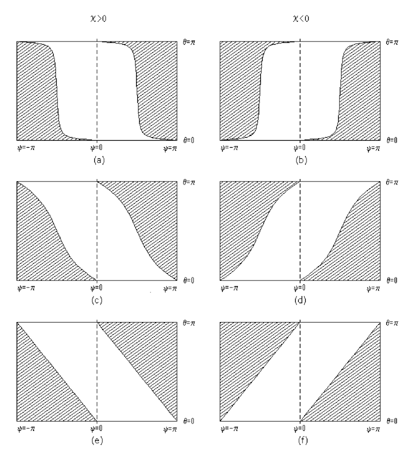
Figure 1: Section of the analyticity domain of ${\cal G}_{E}$ at fixed $\chi$ (white area) for various values of $\chi$: (a) $\chi=0.06$; (b) $\chi=-0.06$; (c) $\chi=0.6$; (d) $\chi=-0.6$; (e) $\chi\to+\infty$; (f) $\chi\to-\infty$.

Sections of this subset at fixed $\chi$ are shown in Fig. 1. The domain “thins out” as one tends towards $\psi\to\pi$ or $\psi\to-\pi$; according to previous works [8, 9, 10, 16, 17, 18], we expect to find the “direct” physical region [i.e., the Minkowskian action of Eq. (20)] at $\theta=0+,\chi>0,\psi=\pi$, and the “crossed” physical region at $\theta=\pi-,\chi<0,\psi=\pi$. This issue will be investigated in the next subsection, where we discuss also what is found at the other edges of the analyticity domain.

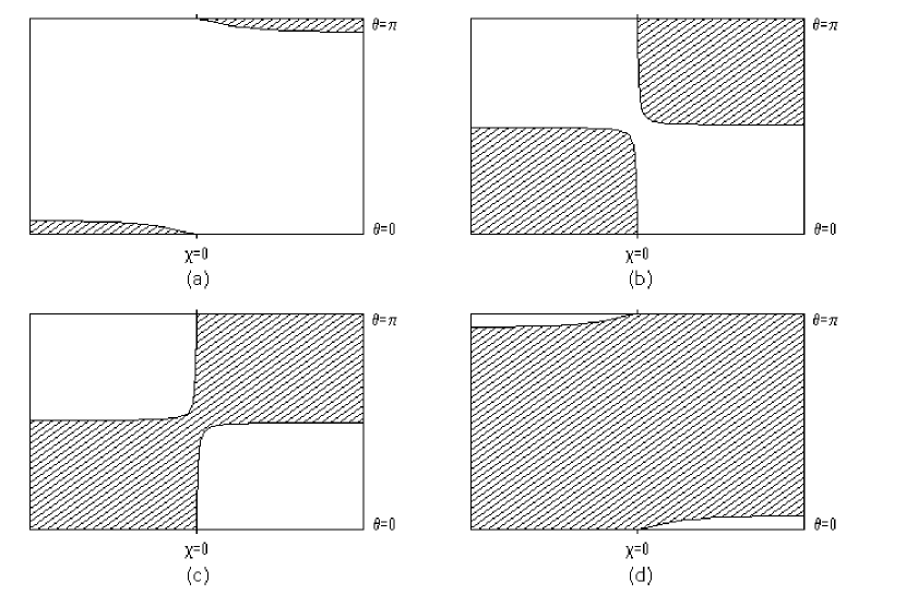
Figure 2: Section of the analyticity domain of ${\cal G}_{E}$ in the $\chi$–$\theta$ plane (white area), for various values of $\psi$: (a) $\psi=0.2$; (b) $\psi=\pi/2-0.02$; (c) $\psi=\pi/2+0.02$; (d) $\psi=\pi-0.2$.

For clarity reasons, and also to make contact with the analysis performed in previous works [8, 9, 10, 16, 17, 18], sections of the same analyticity domain at fixed $\psi$ are shown in Fig. 2: the whole “strip” ${\cal S}_{E}\equiv\{z=\theta-i\chi\,|\,\theta\in(0,\pi),\chi\in\mathbb{R}\}$ (at $\psi=0$) reduces to disjoint regions near the edges of the domain (at $\psi\simeq\pm\pi$).

4.2 Analytic continuation, crossing symmetry and the “reflection relation”

It is convenient to denote the two “physical” edges of the analyticity domain as $E^{\rm dir}$ and $E^{\rm cross}$, with ($z=\theta-i\chi$, $T=|T|e^{i\psi/2}$)

$$E^{\rm dir} =\{(z,T)\in\mathbb{C}^{2}\,|\,\theta=0,\chi\in\mathbb{R}^{+},\psi=\pi\},$$

$$E^{\rm cross} =\{(z,T)\in\mathbb{C}^{2}\,|\,\theta=\pi,\chi\in\mathbb{R}^{-},\psi=\pi\};$$ (41)

it is also convenient to adopt the notation $E^{*}=\{(z,T)\,|\,(z^{*},T^{*})\in E\}$, with which the other two edges of the domain are denoted as $E^{\rm dir}{}^{*}$ and $E^{\rm cross}{}^{*}$.

As we let $\psi\to\pi$ and $\theta\to 0$ (from positive values), approaching $E^{\rm dir}$ from the inside, the coefficients $\overline{C}_{E\mu\nu}$ become imaginary, and

$$\overline{C}_{E\mu\nu}(-i\chi,iT)=i{C}_{M\mu\nu}(\chi,T)$$ (42)

so that

$$S_{E}^{\rm Y.M.}\stackrel{{\scriptstyle\theta\to-i\chi,\,T\to iT}}{{\longrightarrow}}-iS_{M}^{\rm Y.M.},$$ (43)

i.e., according to Eq. (19),

$${\cal G}_{M}(\chi;T;\vec{z}_{\perp};1,2)=\overline{\cal G}_{E}(-i\chi;iT;\vec{z}_{\perp};1,2),\qquad\forall\chi\in\mathbb{R}^{+},T\in\mathbb{R}^{+}.$$ (44)

We thus find that Minkowskian and Euclidean correlation functions are connected by the expected analytic continuation [8, 9, 10, 16], of which we have given here an alternative derivation. More precisely, we can define the analytic extension of the Minkowskian correlation function ${\cal G}_{M}$ from $\chi\in\mathbb{R}^{+},T\in\mathbb{R}^{+}$ to $w\equiv\chi+i\theta=iz$ and complex $T$, by setting

$$\overline{\cal G}_{M}(w;T;\vec{z}_{\perp};1,2)\equiv\overline{\cal G}_{E}(-iw;iT;\vec{z}_{\perp};1,2)\qquad\forall(w,T)\in{\cal D}_{M},$$ (45)

where ${\cal D}_{M}=\{(w,T)\in\mathbb{C}^{2}\,|\,(-iw,iT)\in{\cal D}_{E}\}$, and ${\cal D}_{E}$ has been determined in the previous section, see Eq. (40). The right–hand side of Eq. (45) is indeed the analytic extension of ${\cal G}_{M}$, as the two functions coincide at real positive values of $w$ and real positive $T$, by virtue of Eq. (44). Alternatively, the analytic–continuation relation Eq. (45) for the extended functions can be written as

$$\overline{\cal G}_{E}(z;T;\vec{z}_{\perp};1,2)=\overline{\cal G}_{M}(iz;-iT;\vec{z}_{\perp};1,2),\qquad\forall(z,T)\in{\cal D}_{E}.$$ (46)

From the point of view of the Minkowskian analytically–extended correlation function $\overline{\cal G}_{M}$, the physical axis for the complex angular variable $w=\chi+i\theta$ is approached from above, i.e., from positive imaginary values; as $\chi\simeq\log(s/m^{2})$ at high energies, this corresponds to $\chi+i\epsilon=\log(s/m^{2})+i\epsilon=\log[s/(m-i\epsilon)^{2}]$, in agreement with the usual “$-i\epsilon$” prescription [18].

According to the crossing–symmetry relations (12) (derived in [17]), we should find the physical amplitude in the “crossed” channel at negative values of $\chi$ as $\psi\to\pi$ and $\theta\to\pi$, i.e., at the edge $E^{\rm cross}$ of the analyticity domain. Here we find

$$\overline{C}_{E\mu\nu}(\pi-i\chi,iT)=\sum_{\alpha,\beta=0}^{3}iS_{\mu\alpha}S_{\nu\beta}{C}_{M\alpha\beta}(-\chi,T),$$ (47)

where the matrix $S$ simply interchanges the $0$ and $1$ components of fields and coordinates,

$$S_{\mu\nu}=\left(\begin{array}[]{cccc}0&1&0&0\\ 1&0&0&0\\ 0&0&1&0\\ 0&0&0&1\end{array}\right).$$ (52)

We can reabsorb the matrix $S$ into the loops with a transformation of fields and coordinates, with the only effect of reversing the orientation of $W_{\Gamma_{2}}$, so that $W_{\Gamma_{2}}\to W_{\Gamma_{2}}^{*}$, all the rest remaining unchanged; we thus find that the Euclidean correlation function is analytically continued to the physical correlation function (with positive hyperbolic angle $-\chi$) of a loop and an antiloop, as expected [17]. As a by–product, we reobtain the crossing–symmetry relation for the loops (12), which can now be extended to the whole analyticity domain,

$$\overline{\mathcal{G}}_{M}(i\pi-w;T;\vec{z}_{\perp};1,2) = \overline{\mathcal{G}}_{M}(w;T;\vec{z}_{\perp};1,\overline{2})$$

$$= \overline{\mathcal{G}}_{M}(w;T;\vec{z}_{\perp};\overline{1},2),\quad\forall(w,T)\in{\cal D}_{M},$$

$$\overline{\mathcal{G}}_{E}(\pi-z;T;\vec{z}_{\perp};1,2) = \overline{\mathcal{G}}_{E}(z;T;\vec{z}_{\perp};1,\overline{2})$$ (53)

$$= \overline{\mathcal{G}}_{E}(z;T;\vec{z}_{\perp};\overline{1},2),\quad\forall(z,T)\in{\cal D}_{E},$$

since ${\cal D}_{E}$ satisfies $(z,T)\in{\cal D}_{E}\Leftrightarrow(\pi-z,T)\in{\cal D}_{E}$ [this is easily seen by combining the first two relations of Eq. (32) into $F(\theta,\chi,\psi)=F(\pi-\theta,-\chi,\psi)$], and thus $(w,T)\in{\cal D}_{M}\Leftrightarrow(i\pi-w,T)\in{\cal D}_{M}$.

To see what happens at the other two edges of the analyticity domain it suffices to notice that the domain ${\cal D}_{E}$ possesses the symmetry ${\cal D}_{E}={\cal D}_{E}^{*}$ [see the first relation in Eq. (32)], and that the coefficients $\overline{C}_{E\mu\nu}$ satisfy the reflection relation

$$\overline{C}_{E\mu\nu}(z^{*},T^{*})=\overline{C}_{E\mu\nu}(z,T)^{*}.$$ (54)

We thus find that the correlation function takes conjugate values at conjugate points $(z,T)$ and $(z^{*},T^{*})$, as $C$–invariance (which is not lost when we perform the field transformations) implies that a correlation function does not change if we substitute all the Wilson loops with their antiloops (the notation should be clear):

$$\langle W_{\Gamma_{1}}W_{\Gamma_{2}}\rangle_{S_{E}^{\rm Y.M.}[\overline{C}_{E}(z^{*},T^{*})]}=\langle W_{\Gamma_{1}}W_{\Gamma_{2}}\rangle_{S_{E}^{\rm Y.M.}[\overline{C}_{E}(z,T)^{*}]}=\\ \langle W_{\Gamma_{1}}^{*}W_{\Gamma_{2}}^{*}\rangle_{S_{E}^{\rm Y.M.}[\overline{C}_{E}(z,T)^{*}]}=\langle W_{\Gamma_{1}}W_{\Gamma_{2}}\rangle_{S_{E}^{\rm Y.M.}[\overline{C}_{E}(z,T)]}^{*}$$ (57)

(and similarly for the loop expectation values). We thus conclude that also the correlation function satisfies the reflection relation

$$\overline{\cal G}_{E}(z^{*};T^{*};\vec{z}_{\perp};1,2)=\overline{\cal G}_{E}(z;T;\vec{z}_{\perp};1,2)^{*}.$$ (58)

In particular, this means that at $\psi=-\pi$ we find the complex conjugate of the physical correlation functions, respectively at $E^{\rm dir}{}^{*}$ ($\chi<0$) for the “direct channel” and at $E^{\rm cross}{}^{*}$ ($\chi>0$) for the “crossed channel”. Moreover, from the previous relation we find that the Euclidean correlation function at $\chi=0,\psi=0$ is a real function, as can be shown also in a more direct way making use of the $C$–invariance of the usual Yang–Mills action (this has already been noticed in [23]).

4.3 Analyticity properties of the correlation function with the IR cutoff removed

As the physically relevant quantities are the correlation functions with the IR cutoff removed [11, 16],

$${\cal C}_{M}(\chi;\vec{z}_{\perp};1,2) \equiv\lim_{T\to\infty}{\cal G}_{M}(\chi;T;\vec{z}_{\perp};1,2),$$

$${\cal C}_{E}(\theta;\vec{z}_{\perp};1,2) \equiv\lim_{T\to\infty}{\cal G}_{E}(\theta;T;\vec{z}_{\perp};1,2),$$ (59)

we will discuss now what can be inferred about their analyticity properties from the properties of ${\cal G}_{E}$.

The results of the previous section (see Fig. 1) show that $\overline{\cal G}_{E}$, as a function of the complex variable $T$ at fixed $z=\theta-i\chi$, is analytic in the sector $-\pi/2+\Delta<\arg T=\psi/2<\Delta$, where $\Delta=\Delta(z)\in(0,\pi/2)$. The precise form of $\Delta$ is not needed here, but it can be obtained solving for $\Delta$ the equation $\theta=B(\chi,2\Delta)$, with $B$ defined in Eq. (35). Note that the sector extends on an angle $\pi/2$, irrespectively of $\Delta$ (i.e., of $\theta$ and $\chi$), and that the “strip” $\psi=0$ falls completely inside the domain, so that one can define $I_{\Delta}\equiv(-\pi+2\Delta,2\Delta)$, and rewrite ${\cal D}_{E}$ as ${\cal D}_{E}=\{(z,T)\,|\,z\in{\cal S}_{E},\,\psi\in I_{\Delta(z)}\}$; in the same notation we have ${\cal D}_{M}=\{(w,T)\,|\,w\in{\cal S}_{M},\,\psi\in I_{\Delta(-iw)}-\pi\}$, where ${\cal S}_{M}\equiv i{\cal S}_{E}=\{w=\chi+i\theta\,|\,\chi\in\mathbb{R},\theta\in(0,\pi)\}$ is the Minkowskian “strip”.

A simple nonperturbative argument for the IR finiteness of the normalised correlation function in a non–Abelian gauge theory is as follows. Due to the short–range nature of strong interactions, those parts of the partons’ trajectories that lie too far aside with respect to the “vacuum correlation length” (see Ref. [27] and references therein) do not affect each other; translated in terms of the functional–integral description of the process, this means that there should be a “critical” length $T_{c}$, beyond which the normalised correlation function becomes independent of $T$. Indeed, the available lattice data confirm that ${\cal G}_{E}$ becomes approximately constant for large (real positive) values of $T$ [23]. As the existence of a “vacuum correlation length” is usually ascribed to the non–trivial dynamics dictated by non–Abelian gauge invariance, the previous argument is expected to apply also for the analytically–extended correlation functions, substituting the real variable $T$ with the modulus of the complex variable $|T|$.

In conclusion, the analytically extended correlation function is expected to be analytic and, by the above–mentioned argument, also bounded (at least for large enough $|T|$), as a function of the complex variable $T$, in a sector of the corresponding complex plane, enclosed between two straight lines departing from the origin at an angle $\pi/2$, with finite limits as $|T|\to\infty$ along the two straight lines. We can then apply the Phragmén–Lindelöf theorem (see theorem 5.64 of Ref. [28]) to show that $\overline{\cal G}_{E}$ converges uniformly to a unique value in the whole sector as $|T|\to\infty$, and define unambiguously the functions

$$\overline{\cal C}_{M}(w;\vec{z}_{\perp};1,2) \equiv\lim_{|T|\to\infty}\overline{\cal G}_{M}(w;T;\vec{z}_{\perp};1,2),\qquad\forall w\in{\cal S}_{M}$$

$$\overline{\cal C}_{E}(z;\vec{z}_{\perp};1,2) \equiv\lim_{|T|\to\infty}\overline{\cal G}_{E}(z;T;\vec{z}_{\perp};1,2),\qquad\forall z\in{\cal S}_{E},$$ (60)

since the limit on the right–hand side does not depend on the particular direction in which one performs it. One easily sees that $\overline{\cal C}_{M}$ and $\overline{\cal C}_{E}$ are the analytic extensions of ${\cal C}_{M}$ and of ${\cal C}_{E}$. Indeed, in the Minkowkian case, it suffices to take the limit $|T|\to\infty$ in the equations above setting $w=\chi\in\mathbb{R}^{+}$, as in this case the sector in the complex–$T$ plane, for which $\overline{\cal G}_{M}$ is analytic, extends up to real positive values of $T$. In the Euclidean case, since real positive $T$ are always inside the domain ${\cal D}_{E}$ for every value of the complex angular variable $z=\theta-i\chi$ in the “strip” ${\cal S}_{E}$, one can think of the limit $|T|\to\infty$ as being made along the real axis in the positive direction for every $z$, and it thus suffices to take $z$ to be real, $z=\theta$, and in the interval ${\cal I}_{E}$. If we now take the limit $|T|\to\infty$ in the analytic continuation relations, Eqs. (45) and (46), we obtain the analytic continuation relations with the IR cutoff removed [16],

$$\overline{\cal C}_{M}(w;\vec{z}_{\perp};1,2) = \overline{\cal C}_{E}(-iw;\vec{z}_{\perp};1,2),\qquad\forall w\in{\cal S}_{M},$$

$$\overline{\cal C}_{E}(z;\vec{z}_{\perp};1,2) = \overline{\cal C}_{M}(iz;\vec{z}_{\perp};1,2),\qquad\phantom{-}\forall z\in{\cal S}_{E}.$$ (61)

The crossing–symmetry relations are still valid for $\overline{\cal C}_{M}$ and $\overline{\cal C}_{E}$ throughout the respective analyticity domains ${\cal S}_{M}$ and ${\cal S}_{E}$, as one can prove by taking the limit $|T|\to\infty$ in Eq. (53) (relying again on the Phragmén–Lindelöf theorem mentioned above). Note also that ${\cal C}_{E}(z^{*})={\cal C}_{E}(z)^{*}$ throughout the domain of analyticity, as one can easily see by taking $|T|\to\infty$ in Eq. (58). This conclusion can be reached independently, showing that ${\cal C}_{E}(z)$ is real for real $z$ (as briefly explained at the end of the previous subsection), and using Schwartz’s reflection principle, but in this way no insight on the analyticity domain is obtained.

4.4 Lattice regularisation

As already pointed out, the functional integral must be regularised to become a well–defined mathematical object; here we justify the formal argument given above using a lattice regularisation. In this approach the ill–defined continuum functional integral is replaced with a well–defined (multidimensional) integral, which in the case of gauge theories can be chosen to be an integral on the gauge group manifold [25],

$$\langle{\cal O}[U]\rangle_{S_{\rm lat}}\equiv\dfrac{\displaystyle\int[DU]{\cal O}[U]e^{-S_{\rm lat}[U]}}{\displaystyle\int[DU]e^{-S_{\rm lat}[U]}}$$ (62)

where $DU$ is the invariant Haar measure. The choice of the lattice action $S_{\rm lat}$ is quite arbitrary, and restricted only by gauge invariance and the requirement that in the limit of zero lattice spacing it gives back the desired continuum action. Note that only gauge–invariant operators have non–vanishing expectation value: this means that the case of parton–parton scattering, where the relevant operators are the gauge–dependent Wilson lines, cannot be treated with our approach.

It is easy to see that in our case the action

$$S_{\rm lat}=\beta\sum_{n,\mu<\nu}{C}_{E\mu\nu}(\theta,T)\left[1-\frac{1}{N_{c}}{\rm Re\,}{\rm Tr}U_{\mu\nu}\right],$$ (63)

where $U_{\mu\nu}$ is the usual plaquette variable (in the fundamental representation) [25] and $\beta=2N_{c}/g^{2}$, gives back the action $S_{E}^{\rm Y.M.}$ of Eq. (21) in the limit $a\to 0$, upon identification of the link variables with $U_{\mu}(n)=\exp\{iga\phi_{\mu}(na)\}$. For compact gauge groups, such as $SU(N_{c})$, the integration range is compact, so that, as long as the volume and the lattice spacings are finite, the integral (62) with the action (63) is convergent and analytic in $\theta$ and $T$ ; in the $V\to\infty$ limit, one has to impose positive–definiteness of the real part of the action in order for the integral to remain convergent, and this leads exactly to the convergence conditions studied in the previous section, with which we have determined the analyticity domain of ${\cal G}_{E}$.

The action (63) is correct at tree–level, but one has also to ensure that quantum effects do not modify its form. Before we discuss this point, it is convenient to recall that the Euclidean modified action $S_{E}^{\rm Y.M.}$ has been obtained with independent rescalings of fields and coordinates in the various directions. Indeed, from the definition of $M_{E}$ in Eq. (3) one sees that the coefficients in the action can be written as ${C}_{E\mu\nu}=\lambda_{\mu}^{2}\lambda_{\nu}^{2}/\prod_{\alpha}|\lambda_{\alpha}|$ where $\lambda_{\mu}=M_{E\mu\mu}$, see Eq. (3). It is then easy to see that Eq. (63) is also the correct tree–level action for an anisotropic lattice regularisation of the usual Euclidean Yang–Mills action, as one can directly check [see Eqs. (14) and (3)] by identifying $U_{\mu}(n)=\exp\{iga_{\mu}A_{E\mu}(na)\}$, with $a_{\mu}=a/\lambda_{\mu}$ (note that $\lambda_{\mu}>0$ for $\theta\in{\cal I}_{E}$ and real positive $T$). Showing that Eq. (63) is a good lattice action on an isotropic lattice for the modified action Eq. (21) is then equivalent to show that it is a good action on an anisotropic lattice for the usual Yang–Mills action.

As it has been pointed out in [29], the general anisotropic action is not guaranteed to belong to the same universality class as the isotropic lattice action, and thus one has to enforce that rotation invariance is restored in the continuum limit to get back the usual (Euclidean) Yang–Mills action: in the general case one has to properly tune all the coefficients of the various terms of the action, obtaining in our case

$$\widetilde{S}_{\rm lat}=\sum_{n,\mu<\nu}\beta_{\mu\nu}{C}_{E\mu\nu}(\theta,T)\left[1-\frac{1}{N_{c}}{\rm Re\,}{\rm Tr}U_{\mu\nu}\right],$$ (64)

with properly chosen functions $\beta_{\mu\nu}=\beta_{\mu\nu}(a,\theta,T)$. Due to the asymptotic freedom property of non–Abelian gauge theories, one can determine this functions analytically in perturbation theory for small lattice spacings. One should then check that the coefficients $\beta_{\mu\nu}$ required to restore rotation invariance in the continuum limit do not alter the main results derived in the previous subsections. Quantum effects could in principle impose further restrictions on the analyticity domain ${\cal D}_{E}$ found above, but a preliminary analysis seems to indicate that this is not the case; however, this issue will be discussed in greater detail in a separate publication [30].

We want now to make some remarks on the choice of the operators in the lattice regularisation of Eq. (19). After the field and coordinate transformation, the longitudinal sides of the two continuum Wilson loops are at $45^{\circ}$ with respect to the new axes, and have to be approximated by a broken line (see e.g. Ref. [23]): this introduces approximation errors which have to be carefully considered, but which should vanish in the continuum limit, thus leaving unaltered our analysis. To get rid of this problem, one could use on–axis Wilson loops, thus performing an “exact” calculation on the lattice: to do that one has to perform a further transformation of the action, choosing the new basis vectors along the directions of the longitudinal sides of the loops. The drawback in this case is the appearence of ${\rm Tr}[\Phi_{0\alpha_{\perp}}\Phi_{1\alpha_{\perp}}]$ terms ($\alpha_{\perp}=2,3$), which on the lattice correspond to the more complicated (“chair–like”) terms ${\rm Tr}[U_{0\alpha_{\perp}}U_{1\alpha_{\perp}}^{\dagger}]$.

4.5 Fermions

The full (i.e., not quenched) correlation functions are obtained including fermion effects in the functional integral via the fermion–matrix determinant. We can follow the same approach of the previous subsections also in this case, changing coordinates and fields to push the dependence on the relevant variables $\theta$ and $T$ into the action: the discussion of analyticity properties can then be made along the same lines as in the pure–gauge case, representing the determinant as a functional integral over Grassmann variables and moving derivatives inside the functional integral. The Grassmannian integral can always be performed (at least formally), resulting in a nonlocal functional of the gauge fields; if we assume that the Yang–Mills exponential factor is strong enough to “tame” this functional, as long as the real part of the exponent is positive–definite, the procedure goes on exactly as in the pure Yang–Mills case, and we find the same analyticity structure. Here we shall limit ourselves to the formal argument, and show that the analytic–continuation relations and crossing–symmetry relations remain true also in this case.

Starting from the Euclidean fermionic action and performing the field and coordinate transformation (14), one finds the modified fermionic action, which for $\theta\in(0,\pi)$ and real positive $T$ reads

$$S_{E}^{\rm ferm} =\left(\frac{T}{T_{0}}\right)^{2}\sin\theta\int d^{4}y\bar{\psi}\left({\cal D}_{\mu}M_{E\mu\nu}\gamma_{E\nu}+m\right)\psi,$$ (65)

where ${\cal D}_{\mu}\equiv\frac{\partial}{\partial y^{\mu}}+ig\phi_{\mu}$ and $\gamma_{E0}\equiv\gamma^{0}$, $\gamma_{Ej}\equiv-i\gamma^{j}$, with $\gamma^{\mu}$ the usual Dirac gamma–matrices; the matrix $M_{E}$ is given in Eq. (3). It is then easy to see that the double analytic continuation $\theta\to-i\chi$, $T\to iT$ actually provides the Minkowskian fermionic action, and that the crossing–symmetry relations are reobtained. Indeed, under the analytic continuation ${\cal D}_{\mu}M_{E\mu\nu}\gamma_{E\nu}\to-i{\cal D}_{\mu}M^{\mu}_{\phantom{\mu}\nu}\gamma^{\nu}$, so that

$$S_{E}^{\rm ferm}\to -i\left(\frac{T}{T_{0}}\right)^{2}\sinh\chi\int d^{4}y\bar{\psi}\left(i{\cal D}_{\mu}M^{\mu}_{\phantom{\mu}\nu}\gamma^{\nu}-m\right)\psi$$

$$= -iS_{M}^{\rm ferm},$$ (66)

where $S_{M}^{\rm ferm}$ is the modified Minkwskian action, obtained performing the transformation of fields and coordinates in Minkowski space–time [see Eqs. (13) and (3)], as expected.

The exchanges $\theta\to\pi-\theta$ and $\chi\to i\pi-\chi$ in the Euclidean and Minkowskian theories, respectively, are equivalent to $\phi_{0}\leftrightarrow\phi_{1}$, $y^{0}\leftrightarrow y^{1}$, provided one also performs the following change of variables in the Grassmannian integration,

$$\left\{\begin{aligned} &\psi\to U\psi\\ &\bar{\psi}\to\bar{\psi}U^{\dagger}\end{aligned}\right.$$ (67)

with

$$U=\gamma_{E5}\frac{\gamma_{E0}-\gamma_{E1}}{\sqrt{2}}=\gamma^{5}\frac{\gamma^{0}+i\gamma^{1}}{\sqrt{2}},$$ (68)

where $\gamma_{E5}=\gamma_{E0}\gamma_{E1}\gamma_{E2}\gamma_{E3}=i\gamma^{0}\gamma^{1}\gamma^{2}\gamma^{3}=\gamma^{5}$, in order to exchange also the longitudinal gamma matrices,

$$\left\{\begin{aligned} U^{\dagger}\gamma_{E0}U&=\gamma_{E1},&U^{\dagger}\gamma^{0}U&=-i\gamma^{1}\\ U^{\dagger}\gamma_{E1}U&=\gamma_{E0},&U^{\dagger}\gamma^{1}U&=i\gamma^{0}.\end{aligned}\right.$$ (69)

Note that $U$ is antihermitian and unitary, $U^{\dagger}=-U=U^{-1}$. In this way the exchanges $\theta\to\pi-\theta$ and $\chi\to i\pi-\chi$ are seen to be equivalent to the exchange of one of the two loops with the corresponding antiloop, thus extending the validity of the crossing–symmetry relations (12) to the case where also fermions are included. One can also easily show, combining Eq. (54) and $C$–invariance, that the reflection relation (58) still holds after the inclusion of fermions.

5 Concluding remarks and prospects

In this letter we have approached the analyticity issues related to the problem of soft high–energy scattering by means of functional–integral techniques, giving a nonperturbative justification of the hypotheses underlying the analytic–continuation relations between the relevant Wilson–loop correlation functions in the Euclidean and Minkowskian theories. The argument relies on a transformation of coordinates and fields that moves the whole dependence on the relevant variables, namely the angle $\theta$ between the loops and the half–length $T$, into a modified action; then, the convergence conditions on the functional integral give rise to a nontrivial analyticity domain for the Euclidean correlation function, which is sufficiently wide for the analytic–continuation relations, and also for the crossing–symmetry relations, obtained in [8, 9, 10, 16, 17, 18], to hold; moreover, these relations are reobtained in a completely independent way.

To put the argument on a more solid ground, we have employed a lattice regularisation of the functional integral. Here analyticity of the correlation function follows from the compactness of the integration range as long as the volume and the lattice spacings are finite, and the convergence conditions are necessary conditions for the convergence of the Haar integral in the limit of infinite volume. To ensure the correct continuum limit, the tree–level action should be corrected taking into account quantum effects: in principle this could lead to further restrictions on the domain of analyticity, but a preliminary analysis seems to indicate that this is not the case. This issue will be investigated in greater detail in a separate publication [30]. Also, the infinite–volume limit and the zero–lattice–spacing limit can be sources of singularities if the convergence is not uniform: to prove that this does or does not happen is a very hard problem, which we have not attempted to tackle here. Singularities could also appear if the Wilson–loop expectation value vanishes at some complex value of $\theta$ and $T$: while poles are not a problem for the analytic continuation, the presence of algebraic singularities can cause an ambiguity in the choice of the Riemann sheet.

One can be tempted to take the large–$T$ limit directly in the action, or to perform the analytic continuation from Euclidean to Minkowski space and then take the large–$\chi$ (i.e., high–energy) limit. These limits have to be taken very carefully: for example, if one keeps only the leading order in $T$ (or in $\chi$) in the action of the lattice–regulated functional integral, one obtains exactly zero for both the (unnormalised) correlation function and the Wilson–loop expectation value, leaving the correlation function ${\cal G}_{E}$ undetermined.

The modified Euclidean action derived in section 3 can however be used as a starting point for a nonperturbative investigation of soft high–energy scattering from the first principles of QCD, in principle also from a numerical point of view. This is similar to the approach adopted in Refs. [4, 31, 32], where other rescaled actions have been proposed. This issue (including a detailed study of quantum corrections) will be investigated in another publication [30].

References

- [1] O. Nachtmann, Ann. Phys. 209 (1991) 436.
- [2] H.G. Dosch, in At the frontier of Particle Physics – Handbook of QCD (Boris Ioffe Festschrift), edited by M. Shifman (World Scientific, Singapore, 2001), vol. 2, 1195–1236.
- [3] S. Donnachie, G. Dosch, P. Landshoff and O. Nachtmann, Pomeron Physics and QCD (Cambridge University Press, Cambridge, 2002).
- [4] H. Verlinde and E. Verlinde, hep–th/9302104.
- [5] G.P. Korchemsky, Phys. Lett. B 325 (1994) 459; I.A. Korchemskaya and G.P. Korchemsky, Nucl. Phys. B 437 (1995) 127.
- [6] E. Meggiolaro, Phys. Rev. D 53 (1996) 3835.
- [7] E. Meggiolaro, Nucl. Phys. B 602 (2001) 261.
- [8] E. Meggiolaro, Z. Phys. C 76 (1997) 523.
- [9] E. Meggiolaro, Eur. Phys. J. C 4 (1998) 101.
- [10] E. Meggiolaro, Nucl. Phys. B 625 (2002) 3
- [11] I.I. Balitsky and L.N. Lipatov, Sov. J. Nucl. Phys. 28 (1978) 822; I.I. Balitsky and L.N. Lipatov, JETP Letters 30 (1979) 355.
- [12] H.G. Dosch, E. Ferreira and A. Krämer, Phys. Rev. D 50 (1994) 1992.
- [13] O. Nachtmann, in Perturbative and Nonperturbative aspects of Quantum Field Theory, edited by H. Latal and W. Schweiger (Springer–Verlag, Berlin, Heidelberg, 1997).
- [14] E.R. Berger and O. Nachtmann, Eur. Phys. J. C 7 (1999) 459.
- [15] A.I. Shoshi, F.D. Steffen and H.J. Pirner, Nucl. Phys. A 709 (2002) 131.
- [16] E. Meggiolaro, Nucl. Phys. B 707 (2005) 199.
- [17] M. Giordano and E. Meggiolaro, Phys. Rev. D 74 (2006) 016003.
- [18] E. Meggiolaro, Phys. Lett. B 651 (2007) 177.
- [19] E. Shuryak and I. Zahed, Phys. Rev. D 62 (2000) 085014.
- [20] A.I. Shoshi, F.D. Steffen, H.G. Dosch and H.J. Pirner, Phys. Rev. D 68 (2003) 074004.
- [21] R.A. Janik and R. Peschanski, Nucl. Phys. B 565 (2000) 193.
- [22] R.A. Janik and R. Peschanski, Nucl. Phys. B 586 (2000) 163.
- [23] M. Giordano and E. Meggiolaro, Phys. Rev. D 78 (2008) 074510.
- [24] A. Babansky and I. Balitsky, Phys. Rev. D 67 (2003) 054026.
- [25] K.G. Wilson, Phys. Rev. D 10 (1974) 2445.
- [26] T. Appelquist and W. Fischler, Phys. Lett. B 77 (1978) 405; G. Bhanot, W. Fischler and S. Rudaz, Nucl. Phys. B 155 (1979) 208; M.E. Peskin, Nucl. Phys. B 156 (1979) 365; G. Bhanot and M.E. Peskin, Nucl. Phys. B 156 (1979) 391.
- [27] A. Di Giacomo, H.G. Dosch, V.I. Shevchenko, Yu.A. Simonov, Phys. Rept. 372 (2002) 319; A. Di Giacomo, E. Meggiolaro, H. Panagopoulos, Nucl. Phys. B 483 (1997) 371; M. D’Elia, A. Di Giacomo, E. Meggiolaro, Phys. Lett. B 408 (1997) 315.
- [28] E.C. Titchmarsh, The Theory of Functions, 2nd edition (Cambridge University Press, London, 1939).
- [29] G. Burgio, A. Feo, M.J. Peardon, S.M. Ryan, Phys. Rev. D 67 (2003) 114502.
- [30] M. Giordano and E. Meggiolaro, in preparation.
- [31] I.Ya. Aref’eva, Phys. Lett. B 325 (1994) 171; I.Ya. Aref’eva, Phys. Lett. B 328 (1994) 411.
- [32] P. Orland and J. Xiao, arXiv:0901.2955 [hep-ph].